Fast Bayesian Non-Negative Matrix Factorisation and Tri-Factorisation

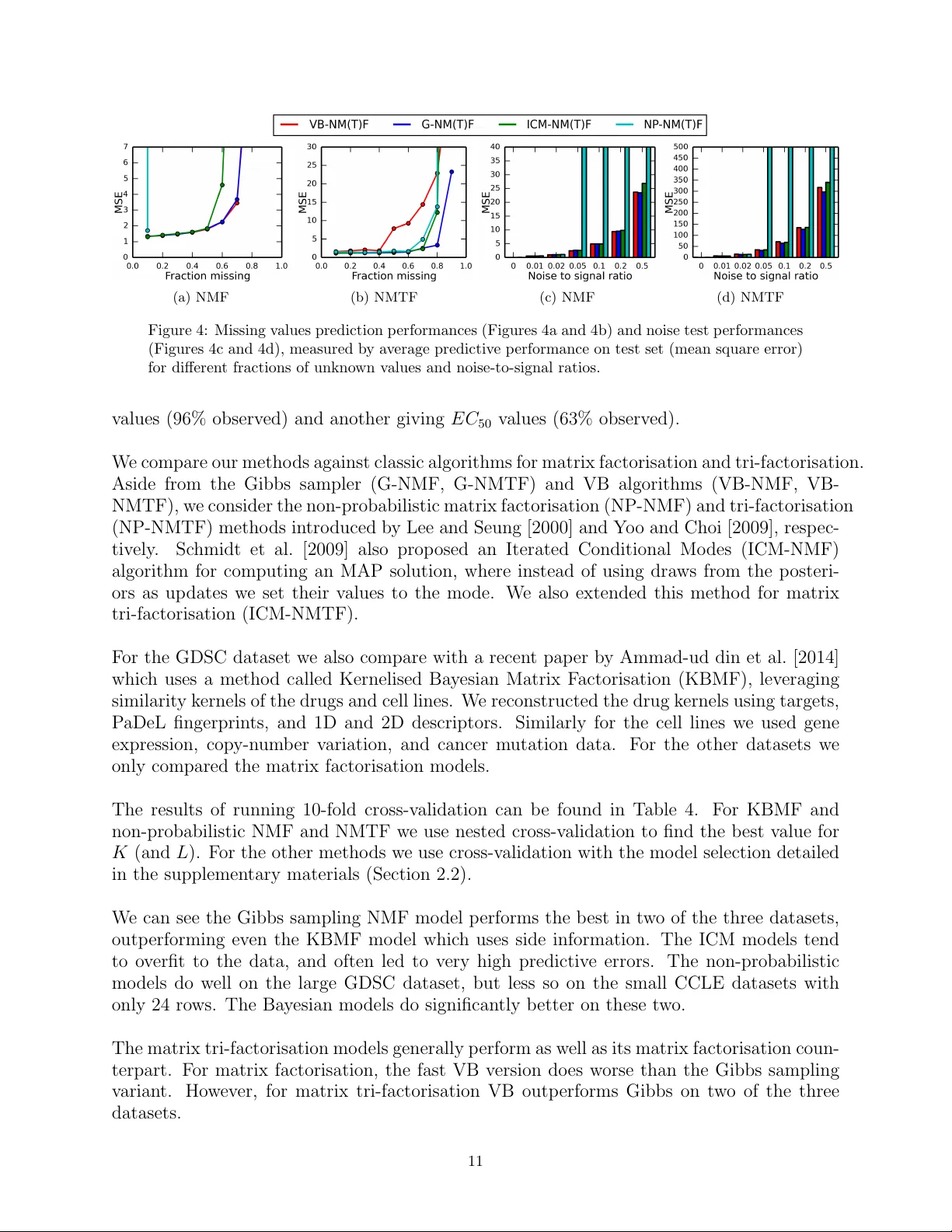
F ast Bayesian Non-Negati ve Matrix F actorisation and T ri-F actorisation Thomas Brouwer Computer Laboratory Univ ersity of Cambridge United Kingdom tab43@cam.ac.uk Jes Fr ellsen Department of Engineering Univ ersity of Cambridge United Kingdom jf519@cam.ac.uk Pietro Lio’ Computer Laboratory Univ ersity of Cambridge United Kingdom pl219@cam.ac.uk Abstract W e present a fast v ariational Bayesian algorithm for performing non-negati ve matrix factorisation and tri-factorisation. W e show that our approach achiev es faster con vergence per iteration and timestep (w all-clock) than Gibbs sampling and non-probabilistic approaches, and do not require additional samples to estimate the posterior . W e show that in particular for matrix tri-factorisation con ver gence is difficult, b ut our variational Bayesian approach of fers a fast solution, allo wing the tri-factorisation approach to be used more ef fectiv ely . 1 Introduction Non-negati ve matrix factorisation methods Lee and Seung [1999] hav e been used extensi vely in recent years to decompose matrices into latent factors, helping us reveal hidden structure and predict missing values. In particular we decompose a giv en matrix into two smaller matrices so that their product approximates the original one. The non-negati vity constraint makes the resulting matrices easier to interpret, and is often inherent to the problem – such as in image processing or bioinformatics (Lee and Seung [1999], W ang et al. [2013]). Some approaches approximate a maximum lik elihood (ML) or maximum a posteriori (MAP) solution that minimises the dif ference between the observed matrix and the decomposition of this matrix. This gives a single point estimate, which can lead to ov erfitting more easily and neglects uncertainty . Instead, we may wish to find a full distribution ov er the matrices using a Bayesian approach, where we define prior distrib utions ov er the matrices and then compute their posterior after observing the actual data. Schmidt et al. [2009] presented a Bayesian model for non-negativ e matrix f actorisation that uses Gibbs sampling to obtain draws of these posteriors, with e xponential priors to enforce non-ne gativity . Markov chain Monte Carlo (MCMC) methods like Gibbs sampling rely on a sampling procedure to ev entually con ver ge to draws of the desired distrib ution – in this case the posterior of the matrices. This means that we need to inspect the values of the draws to determine when our method has con ver ged (burn-in), and then take additional dra ws to estimate the posteriors. W e present a variational Bayesian approach to non-negati ve matrix factorisation, where instead of relying on random draws we obtain a deterministic con vergence to a solution. W e do this by introducing a new distribution that is easier to compute, and optimise it to be as similar to the true posterior as possible. W e sho w that our approach gi ves faster con vergence rates per iteration and timestep (wall-clock) than current methods, and is less prone to overfitting than the popular non-probabilistic approach of Lee and Seung [2000]. W e also consider the problem of non-negati ve matrix tri-factorisation, first introduced by Ding et al. [2006], where we decompose the observed dataset into three smaller matrices, which again are constrained to be non-negati ve. Matrix tri-factorisation has been explored extensi vely in recent years, for example for collaborative filtering (Chen et al. [2009]) and clustering genes and phenotypes 30th Conference on Neural Information Processing Systems (NIPS 2016), Barcelona, Spain. (Hwang et al. [2012]). W e present a fully Bayesian model for non-negati ve matrix tri-factorisation, extending the matrix f actorisation model to obtain both a Gibbs sampler and a v ariational Bayesian algorithm for inference. W e show that con ver gence is ev en harder , and that the variational approach provides significant speedups (roughly four times faster) compared to Gibbs sampling. 2 Non-Negative Matrix F actorisation W e follo w the notation used by Schmidt et al. [2009] for non-negati ve matrix f actorisation (NMF), which can be formulated as decomposing a matrix R ∈ R I × J into two latent (unobserved) matrices U ∈ R I × K + and V ∈ R J × K + . In other words, solving R = U V T + E , where noise is captured by matrix E ∈ R I × J . The dataset R need not be complete – the indices of observed entries can be represented by the set Ω = { ( i, j ) | R ij is observed } . These entries can then be predicted by U V T . W e take a probabilistic approach to this problem. W e express a likelihood function for the observ ed data, and treat the latent matrices as random variables. As the likelihood we assume each value of R comes from the product of U and V , with some Gaussian noise added, R ij ∼ N ( R ij | U i · V j , τ − 1 ) where U i , V j denote the i th and j th rows of U and V , and N ( x | µ, τ ) is the density of the Gaussian distribution, with precision τ . The full set of parameters for our model is denoted θ = { U , V , τ } . In the Bayesian approach to inference, we want to find the distrib utions ov er the parameters θ after observing the data D = { R ij } i,j ∈ Ω . W e can use Bayes’ theorem for this, p ( θ | D ) ∝ p ( D | θ ) p ( θ ) . W e need priors over the parameters, allo wing us to express beliefs for their values – such as constraining U , V to be non-negati ve. W e can normally not compute the posterior p ( θ | D ) exactly , but some choices of priors allow us to obtain a good approximation. Schmidt et al. choose an exponential prior ov er U and V , so that each element in U and V is assumed to be independently exponentially distributed with rate parameters λ U ik , λ V j k > 0 , U ik ∼ E ( U ik | λ U ik ) V j k ∼ E ( V j k | λ V j k ) where E ( x | λ ) is the density of the exponential distribution. For the precision τ we use a Gamma distribution with shape α > 0 and rate β > 0 . Schmidt et al. [2009] introduced a Gibbs sampling algorithm for approximating the posterior distri- bution, which relies on sampling ne w values for each random variable in turn from the conditional posterior distribution. Details on this method can be found in t he supplementary materials (Section 1.1). V ariational Bayes for NMF Like Gibbs sampling, v ariational Bayesian inference (VB) is a w ay to approximate the true posterior p ( θ | D ) . The idea behind VB is to introduce an approximation q ( θ ) to the true posterior that is easier to compute, and to make our v ariational distribution q ( θ ) as similar to p ( θ | D ) as possible (as measured by the KL-di ver gence). W e assume the variational distrib ution q ( θ ) factorises completely , so all v ariables are independent, q ( θ ) = Q θ i ∈ θ q ( θ i ) . This is called the mean-field assumption. W e assume the same forms of q ( θ i ) as used in Gibbs sampling, q ( τ ) = G ( τ | α ∗ , β ∗ ) q ( U ik ) = T N ( U ik | µ U ik , τ U ik ) q ( V j k ) = T N ( V j k | µ V j k , τ V j k ) Beal and Ghahramani [2003] showed that the optimal distrib ution for the i th parameter , q ∗ ( θ i ) , can be expressed as follo ws (for some constant C ), allo wing us to find the optimal updates for the v ariational parameters log q ∗ ( θ i ) = E q ( θ − i ) [log p ( θ , D )] + C. Note that we take the expectation with respect to the distrib ution q ( θ − i ) ov er the parameters b ut excluding the i th one. This giv es rise to an iterativ e algorithm: for each parameter θ i we update its distribution to that of its optimal v ariational distribution, and then update the e xpectation and v ariance with respect to q . This algorithm is guaranteed to maximise the Evidence Lower Bound (ELBO) L = E q [log p ( θ , D ) − log q ( θ )] , which is equiv alent to minimising the KL-div ergence. More details and updates for the approximate posterior distribution parameters are gi ven in the supplementary materials (Section 1.2). 2 3 Non-Negative Matrix T ri-Factorisation The problem of non-negati ve matrix tri-f actorisation (NMTF) can be formulated similarly to that of non-negati ve matrix factorisation. W e now decompose our dataset R ∈ R I × J into three matrices F ∈ R I × K + , S ∈ R K × L + , G ∈ R J × L + , so that R = F S G T + E . W e again use a Gaussian lik elihood and Exponential priors for the latent matrices. R ij ∼ N ( R ij | F i · S · G j , τ − 1 ) τ ∼ G ( τ | α, β ) F ik ∼ E ( F ik | λ F ik ) S kl ∼ E ( S kl | λ S kl ) G j l ∼ E ( G j l | λ G j l ) A Gibbs sampling algorithm that can be deriv ed similarly to before. Details can be found in the supplementary materials (Section 1.3). 3.1 V ariational Bayes for NMTF Our VB algorithm for tri-factorisation follows the same steps as before, but now has an added complexity due to the term E q  ( R ij − F i · S · G j ) 2  . Before, all covariance terms for k 0 6 = k were zero due to the factorisation in q , but we no w obtain some additional non-zero cov ariance terms. This leads to the more complicated variational updates gi ven in the supplementary materials (Section 1.4). E q  ( R ij − F i · S · G j ) 2  = R ij − K X k =1 L X l =1 f F ik f S kl g G j l ! 2 + K X k =1 L X l =1 V ar q [ F ik S kl G j l ] + K X k =1 L X l =1 X k 0 6 = k Co v [ F ik S kl G j l , F ik 0 S k 0 l G j l ] + K X k =1 L X l =1 X l 0 6 = l Co v [ F ik S kl G j l , F ik S kl 0 G j l 0 ] 4 Experiments T o demonstrate the performances of our proposed methods, we ran sev eral experiments on a toy dataset, as well as sev eral drug sensitivity datasets. For the toy dataset we generated the latent matrices using unit mean exponential distributions, and adding zero mean unit v ariance Gaussian noise to the resulting product. For the matrix factorisation model we use I = 100 , J = 80 , K = 10 , and for the matrix tri-factorisation I = 100 , J = 80 , K = 5 , L = 5 . W e also consider a drug sensiti vity dataset, which detail the ef fectiv eness of different drugs on cell lines for cancer and tissue types. The Genomics of Drug Sensitivity in Cancer (GDSC v5.0, Y ang et al. [2013]) dataset contains 138 drugs and 622 cell lines, with 81% of entries observed. W e compare our methods against classic algorithms for matrix factorisation and tri-factorisation. Aside from the Gibbs sampler (G-NMF , G-NMTF) and VB algorithms (VB-NMF , VB-NMTF), we consider the non-probabilistic matrix factorisation (NP-NMF) and tri-factorisation (NP-NMTF) methods introduced by Lee and Seung [2000] and Y oo and Choi [2009], respecti vely . Schmidt et al. [2009] also proposed an Iterated Conditional Modes (ICM-NMF) algorithm for computing an MAP solution, where instead of using draws from the posteriors as updates we set their v alues to the mode. W e also extended this method for matrix tri-f actorisation (ICM-NMTF). 4.1 Con vergence speed W e tested the con vergence speed of the methods on both the toy data, giving the correct v alues for K, L , and on the GDSC drug sensitivity dataset. W e track the con ver gence rate of the error (mean square error) on the training data against the number of iterations tak en. This can be found for the toy data in Figures 1a (MF) and 1b (MTF), and for the GDSC drug sensitivity dataset in Figures 1c and 1d. Below that (Figures 1e-1h) is the con vergence in terms of time (w all-clock), timing each run 10 times and taking the av erage (using the same random seed). W e see that our VB methods takes the fewest iterations to con ver ge to the best solution. This is especially the case in the tri-factorisation case, where the best solution is much harder to find (note that all methods initially find a worse solution and get stuck on that for a while), and our v ariational approach con ver ges sev en times faster in terms of iterations taken. W e note that time wise, the ICM 3 (a) T o y NMF (b) T o y NMTF (c) Drug sensiti vity NMF (d) Drug sensiti vity NM TF (e) T o y NMF (f) T o y NMTF (g) Drug sensiti vity NMF (h) Drug sensiti vity NMTF Figure 1: Con v er gence of algorithms on the to y and GDSC drug sensiti vity datasets, measuring the training data fit (mean square error) across iterations (top ro w) and time (bottom ro w). (a) NMF (b) NMTF (c) NMF (d) NMTF Figure 2: Missing v alues prediction performances (Figures 2a and 2b) and noise test performances (Figures 2c and 2d), measured by a v erage predi cti v e performance on test set (mean square error) for dif ferent fractions of unkno wn v alues and noise-to-signal ratios. algorithms can be implemented more ef fi ciently than the fully Bayesian approaches, b ut returns a MAP solution rather than the full posterior . Our VB method still con v er ges four times f aster than the other fully Bayesian approach, and twice as f ast as the non-probabilistic method. 4.2 Other experiments W e conducted se v eral other e xperiments, such as model selection on to y datasets, and cross-v alidation on three drug sensiti vity dat asets. Details and results for all e xperiments are gi v en in the supplementary materials (Section 3), b ut here we highlight the results for missing v alue predictions and noise tests. In Figures 2a and 2b, we measure the ability of the models to predict missing v alues in a to y dataset as the fraction of missing v alues increases. Similarly , Figures 2c and 2d sho w the predicti v e performances as the amount of noise in the data increases. The figures sho w that the Bayesian models are more rob ust to noise, and perform better on sparse datasets than their non-probabilistic counterparts. 5 Conclusion W e ha v e introduced a f ast v ariational Bayesian algorithm for performing non-ne g ati v e matrix f actori- sation and tri-f actorisati on. W e ha v e sho wn that this method gi v es us deterministic con v er gence that is f aster than MCMC methods, without requiring additional samples to estimate the posterior distri- b ution. W e demonstrate that our v ariational approach is particularly useful for the tri-f actorisation case, where con v er gence is e v en harder , and we obtain a four -fold time speedup. These speedups can open up the applicability of the models to lar ger datasets. 4 Acknowledgement This work was supported by the UK Engineering and Physical Sciences Research Council (EPSRC), grant reference EP/M506485/1. JF acknowledge funding from the Danish Council for Independent Research 0602-02909B. References M. Ammad-ud din, E. Georgii, M. Gönen, T . Laitinen, O. Kallioniemi, K. W ennerber g, A. Poso, and S. Kaski. Integrativ e and personalized QSAR analysis in cancer by kernelized Bayesian matrix factorization. J ournal of chemical information and modeling , 54(8):2347–59, Aug. 2014. J. Barretina, G. Caponigro, N. Stransky , K. V enkatesan, A. A. Margolin, S. Kim, C. J. W ilson, et al. The Cancer Cell Line Encyclopedia enables predicti ve modelling of anticancer drug sensiti vity. Natur e , 483(7391):603–7, Mar . 2012. M. Beal and Z. Ghahramani. The V ariational Bayesian EM Algorithm for Incomplete Data: with Application to Scoring Graphical Model Structures. Bayesian Statistics 7, Oxfor d University Pr ess , 2003. G. Chen, F . W ang, and C. Zhang. Collaborativ e filtering using orthogonal nonnegati ve matrix tri-factorization. Information Pr ocessing and Manag ement , 45(3):368–379, May 2009. C. Ding, T . Li, W . Peng, and H. P ark. Orthogonal nonnegati ve matrix t-factorizations for clustering. In Pr oceedings of the 12th A CM SIGKDD , pages 126–135, Ne w Y ork, Ne w Y ork, USA, Aug. 2006. A CM Press. T . Hwang, G. Atluri, M. Xie, S. De y , C. Hong, V . Kumar , and R. K uang. Co-clustering phenome- genome for phenotype classification and disease gene discov ery. Nucleic Acids Researc h , 40(19): e146, Oct. 2012. D. D. Lee and H. S. Seung. Learning the parts of objects by non-ne gativ e matrix factorization. Natur e , 401(6755):788–791, Oct. 1999. D. D. Lee and H. S. Seung. Algorithms for Non-negati ve Matrix Factorization. NIPS, MIT Press , pages 556–562, 2000. M. N. Schmidt, O. W inther , and L. K. Hansen. Bayesian non-negativ e matrix factorization. In Independent Component Analysis and Signal Separation, International Confer ence on (ICA), Springer Lecture Notes in Computer Science, V ol. 5441 , pages 540–547, 2009. B. Seashore-Ludlo w , M. G. Rees, J. H. Cheah, M. Cokol, E. V . Price, M. E. Coletti, V . Jones, et al. Harnessing Connecti vity in a Large-Scale Small-Molecule Sensiti vity Dataset. Cancer discovery , 5(11):1210–23, Nov . 2015. J. J.-Y . W ang, X. W ang, and X. Gao. Non-negati ve matrix f actorization by maximizing correntropy for cancer clustering. BMC bioinformatics , 14(1):107, Jan. 2013. W . Y ang, J. Soares, P . Greninger, E. J. Edelman, H. Lightfoot, S. F orbes, N. Bindal, D. Beare, J. A. Smith, I. R. Thompson, S. Ramaswamy , P . A. Futreal, D. A. Haber , M. R. Stratton, C. Benes, U. McDermott, and M. J. Garnett. Genomics of Drug Sensitivity in Cancer (GDSC): a resource for therapeutic biomarker disco very in cancer cells. Nucleic acids r esear ch , 41(Database issue): D955–61, Jan. 2013. J. Y oo and S. Choi. Probabilistic matrix tri-factorization. In IEEE International Confer ence on Acoustics, Speech, and Signal Pr ocessing , number 3, pages 1553–1556. IEEE, Apr . 2009. 5 F ast Ba y esian Non-Negativ e Matrix F actorisation and T ri-F actorisation Supplemen tary Materials Thomas Brou wer, Jes F rellsen, Pietro Lio’ Univ ersity of Cambridge Submitted to NIPS 2016 W orkshop – Adv ances in Appro ximate Ba yesian Inference. Con ten ts 1 Mo del details 2 1.1 Gibbs sampling for matrix factorisation . . . . . . . . . . . . . . . . . . . . . 2 1.2 V ariational Bay es for matrix factorisation . . . . . . . . . . . . . . . . . . . . 3 1.3 BNMTF Gibbs sampling parameter v alues . . . . . . . . . . . . . . . . . . . 3 1.4 BNMTF V ariational Bay es parameter up dates . . . . . . . . . . . . . . . . . 4 2 Mo del discussion 6 2.1 Complexit y . . . . . . . . . . . . . . . . . . . . . . . . . . . . . . . . . . . . 6 2.2 Mo del selection . . . . . . . . . . . . . . . . . . . . . . . . . . . . . . . . . . 6 2.3 Initialisation . . . . . . . . . . . . . . . . . . . . . . . . . . . . . . . . . . . . 7 2.4 Implemen tation . . . . . . . . . . . . . . . . . . . . . . . . . . . . . . . . . . 7 2.5 Co de . . . . . . . . . . . . . . . . . . . . . . . . . . . . . . . . . . . . . . . . 8 3 Additional exp erimen ts 9 3.1 Mo del selection . . . . . . . . . . . . . . . . . . . . . . . . . . . . . . . . . . 9 3.2 Missing v alues . . . . . . . . . . . . . . . . . . . . . . . . . . . . . . . . . . . 10 3.3 Noise test . . . . . . . . . . . . . . . . . . . . . . . . . . . . . . . . . . . . . 10 3.4 Drug sensitivit y predictions . . . . . . . . . . . . . . . . . . . . . . . . . . . 10 1 1 Mo del details 1.1 Gibbs sampling for matrix factorisation In this section we offer an introduction to Gibbs sampling, and show ho w it can b e applied to the Ba yesian non-negative matrix factorisation mo del. Gibbs sampling w orks b y sampling new v alues for eac h parameter θ i from its marginal distri- bution giv en the current v alues of the other parameters θ − i , and the observed data D . If we sample new v alues in turn for eac h parameter θ i from p ( θ i | θ − i , D ), w e will even tually con- v erge to dra ws from the p osterior, which can b e used to approximate the p osterior p ( θ | D ). W e ha ve to discard the first n dra ws b ecause it takes a while to con v erge ( burn-in ), and since consecutiv e draws are correlated we only use every i th v alue ( thinning ). F or the Ba y esian non-negativ e matrix factorisation mo del this means that we need to b e able to dra w from the following distributions: p ( U ik | τ , U − ik , V , D ) p ( V j k | τ , U , V − j k , D ) p ( τ | U , V , D ) where U − ik denotes all elemen ts in U except U ik , and similarly for V − j k . Using Bay es theorem w e can obtain the p osterior distributions. F or example, for p ( U ik | τ , U − ik , V , D ): p ( U ik | τ , U − ik , V , D ) ∝ p ( D | τ , U , V ) × p ( U ik | λ U ik ) ∝ Y j ∈ Ω i N ( R ij | U i · V j , τ − 1 ) × E ( U ik | λ U ik ) ∝ exp ( τ 2 X j ∈ Ω i ( R ij − U i · V j ) 2 ) × exp  − λ U ik U ik  × u ( x ) ∝ exp ( U 2 ik 2 " τ X j ∈ Ω i V 2 j k # + U ik " − λ U ik + τ X j ∈ Ω i ( R ij − X k 0 6 = k U ik 0 V j k 0 ) V j k #) × u ( x ) ∝ exp  τ U ik 2 ( U ik − µ U ik ) 2  × u ( x ) ∝ T N ( U ik | µ U ik , τ U ik ) where T N ( x | µ, τ ) =    p τ 2 π exp  − τ 2 ( x − µ ) 2  1 − Φ( − µ √ τ ) if x ≥ 0 0 if x < 0 is a truncated normal: a normal distribution with zero densit y b elow x = 0 and renormalised to in tegrate to one. Φ( · ) is the cumulativ e distribution function of N (0 , 1). Applying the same tec hnique to the other p osteriors gives us: p ( τ | U , V , D ) = G ( τ | α ∗ , β ∗ ) p ( V j k | τ , U , V − j k , D ) = T N ( V j k | µ V j k , τ V j k ) The parameters of these distributions are giv en in T able 1, where Ω i = { j | ( i, j ) ∈ Ω } and Ω j = { i | ( i, j ) ∈ Ω } . 2 T able 1: NMF v ariable update rules GIBBS SAMPLING V ARIA TIONAL BA YES α ∗ α + | Ω | 2 α + | Ω | 2 β ∗ β + 1 2 X ( i,j ) ∈ Ω ( R ij − U i · V j ) 2 β + 1 2 P ( i,j ) ∈ Ω E q h ( R ij − U i V j ) 2 i τ U ik τ X j ∈ Ω i V 2 j k e τ P j ∈ Ω i g V 2 j k µ U ik 1 τ U ik   − λ U ik + τ X j ∈ Ω i ( R ij − X k 0 6 = k U ik 0 V j k 0 ) V j k   1 τ U ik  − λ U ik + e τ P j ∈ Ω i  R ij − P k 0 6 = k g U ik 0 g V j k 0  g V j k  τ V j k τ X i ∈ Ω j U 2 ik τ P i ∈ Ω j g U 2 ik µ V j k 1 τ V j k   − λ V j k + τ X i ∈ Ω j ( R ij − X k 0 6 = k U ik 0 V j k 0 ) U ik   1 τ V j k  − λ V j k + e τ P i ∈ Ω j  R ij − P k 0 6 = k g U ik 0 g V j k 0  g U ik  E q h ( R ij − U i V j ) 2 i = R ij − K X k =1 g U ik g V j k ! 2 + K X k =1  g U 2 ik g V 2 j k − g U ik 2 g V j k 2  1.2 V ariational Ba y es for matrix factorisation F or the V ariational Ba y es algorithm for inference, up dates for the approximate p osterior distributions are giv en in T able 1, and were obtained using the tec hniques describ ed in the pap er. W e use ] f ( X ) as a shorthand for E q [ f ( X )], where X is a random v ariable and f is a function o ver X . W e mak e use of the iden tit y f X 2 = e X 2 + V ar q [ X ]. The exp ectation and v ariance of the parameters with resp ect to q are giv en b elo w, for random v ariables X ∼ G ( a, b ) and Y ∼ T N ( µ, τ ). e X = a b e Y = µ + 1 √ τ λ  − µ √ τ  V ar [ Y ] = 1 τ  1 − δ  − µ √ τ  where ψ ( x ) = d dx log Γ( x ) is the digamma function, λ ( x ) = φ ( x ) / [1 − Φ( x )], and δ ( x ) = λ ( x )[ λ ( x ) − x ]. φ ( x ) = 1 √ 2 π exp {− 1 2 x 2 } is the densit y function of N (0 , 1). 1.3 BNMTF Gibbs sampling parameter v alues F or the BNMTF Gibbs sampling algorithm, we sample from the following p osteriors: p ( τ | F , S , G , D ) = G ( τ | α ∗ , β ∗ ) p ( F ik | τ , F − ik , S , G , D ) = T N ( F ik | µ F ik , τ F ik ) p ( S kl | τ , F , S − kl , G , D ) = T N ( S kl | µ S kl , τ S kl ) p ( G j l | τ , F , S , G − j l , D ) = T N ( G j l | µ G j l , τ G j l ) 3 The up dates for the parameters are giv en in T able 2 b elo w. T able 2: NMTF Gibbs Up date Rules GIBBS SAMPLING α ∗ α + | Ω | 2 β ∗ β + 1 2 X ( i,j ) ∈ Ω ( R ij − F i · S · G j ) 2 τ F ik τ X j ∈ Ω i ( S k · G j ) 2 µ F ik 1 τ F ik   − λ F ik + τ X j ∈ Ω i   R ij − X k 0 6 = k L X l =1 F ik 0 S k 0 l G j l   ( S k · G j )   τ S kl τ X ( i,j ) ∈ Ω F 2 ik G 2 j l µ S kl 1 τ S kl   − λ S kl + τ X ( i,j ) ∈ Ω   R ij − X ( k 0 ,l 0 ) 6 =( k,l ) F ik 0 S k 0 l 0 G j l 0   F ik G j l   τ G j l τ X i ∈ Ω j ( F i · S · ,l ) 2 µ G j l 1 τ G j l   − λ G j l + τ X i ∈ Ω j   R ij − K X k =1 X l 0 6 = l F ik S kl 0 G j l 0   ( F i · S · ,l )   1.4 BNMTF V ariational Ba y es parameter up dates As discussed in the pap er, the term E q  ( R ij − F i · S · G j ) 2  adds extra complexity to the matrix tri-factorisation case. E q  ( R ij − F i · S · G j ) 2  = R ij − K X k =1 L X l =1 f F ik f S kl f G j l ! 2 + K X k =1 L X l =1 V ar q [ F ik S kl G j l ] (1) + K X k =1 L X l =1 X k 0 6 = k Co v [ F ik S kl G j l , F ik 0 S k 0 l G j l ] (2) + K X k =1 L X l =1 X l 0 6 = l Co v [ F ik S kl G j l , F ik S kl 0 G j l 0 ] (3) 4 The ab o ve v ariance and co v ariance terms are equal to the following, resp ectiv ely: f F 2 ik f S 2 kl f G 2 j l − f F ik 2 f S kl 2 f G j l 2 (1) V ar q [ F ik ] f S kl f G j l g S kl 0 g G j l 0 (2) f F ik f S kl V ar q [ G j l ] g F ik 0 g S k 0 l (3) The up dates for the v ariational parameters of the V ariational Bay es algorithm for the Ba yesian non-negative matrix tri-factorisation are given in T able 3 b elo w. T able 3: NMTF VB Up date Rules V ARIA TIONAL BA YES α ∗ α + | Ω | 2 β ∗ β + 1 2 X ( i,j ) ∈ Ω E q h ( R ij − F i · S · G j ) 2 i τ F ik e τ X j ∈ Ω i   L X l =1 f S kl g G j l ! 2 + L X l =1  f S 2 kl g G 2 j l − f S kl 2 g G j l 2    µ F ik 1 τ F ik   − λ F ik + e τ X j ∈ Ω i     R ij − X k 0 6 = k L X l =1 g F ik 0 g S k 0 l g G j l   L X l =1 f S kl g G j l − L X l =1 f S kl V ar q [ G j l ] X k 0 6 = k g F ik 0 g S k 0 l     τ S kl e τ X ( i,j ) ∈ Ω f F 2 ik g G 2 j l µ S kl 1 τ S kl   − λ S kl + e τ X ( i,j ) ∈ Ω     R ij − X ( k 0 ,l 0 ) 6 =( k,l ) g F ik 0 g S k 0 l 0 g G j l 0   f F ik g G j l − f F ik V ar q [ G j l ] X k 0 6 = k g F ik 0 g S k 0 l − V ar q [ F ik ] g G j l X l 0 6 = l g S kl 0 g G j l 0     τ G j l e τ X i ∈ Ω j   K X k =1 f F ik f S kl ! 2 + K X k =1  f F 2 ik f S 2 kl − f F ik 2 f S kl 2    µ G j l 1 τ G j l   − λ G j l + e τ X i ∈ Ω j     R ij − K X k =1 X l 0 6 = l f F ik g S kl 0 g G j l 0   K X k =1 f F ik f S kl − K X k =1 V ar q [ F ik ] f S kl X l 0 6 = l g S kl 0 g G j l 0     5 2 Mo del discussion 2.1 Complexit y The updates for the Gibbs samplers and VB algorithms can b e implemen ted efficien tly us- ing matrix op erations. The time complexit y p er iteration for Ba y esian non-negative matrix factorisation is O ( I J K 2 ) for b oth Gibbs and VB, and O ( I J ( K 2 L + K L 2 )) per iteration for tri-factorisation. Ho wev er, the up dates in eac h column of U , V , F , G are indep enden t of eac h other and can therefore b e up dated in parallel. F or the Gibbs sampler, this means w e can draw these v alues in parallel, but for the VB algo- rithm w e can join tly up date the columns using a single matrix op eration. Mo dern computer arc hitectures can exploit this using vector pro cessors, leading to a great sp eedup. F urthermore, after the VB algorithm conv erges w e ha v e our appro ximation to the poste- rior distributions immediately , whereas with Gibbs w e need to obtain further draws after con vergence and use a thinning rate to obtain an accurate estimate of the p osterior. This deterministic b ehaviour of VB mak es it easier to use. Although additional v ariables need to b e stored to represent the p osteriors, this do es not result in a w orse space complexit y , as the Gibbs sampler needs to store dra ws ov er time. 2.2 Mo del selection In practice w e do not know the optimal mo del dimensionality of our data, and w e need to estimate its v alue. In our case, w e wan t to find the b est v alue of K for matrix factorisation, and K, L for tri-factorisation. The log probabilit y of the data, log p ( D | θ ), is a go o d measure for the quality of the fit to the data. As K increases w e exp ect the log likelihoo d to improv e as we giv e the mo del more freedom for fitting to the data, but this can lead to o v erfitting. Therefore, w e need to p enalise the mo del’s p erformance by its complexit y . W e use the Ak aike information criterion (AIC) Ak aike [1974] defined as AI C = 2 k − 2 log p ( D | θ ) where k is the num b er of free parameters in our mo del. F or matrix factorisation this is I K + J K and for tri-factorisation I K + K L + J L . Another popular measure is the Bay esian information criterion (BIC) Sch w arz [1978]. BIC tends to p enalise complicated mo dels more hea vily than AIC. W e found that AIC p eaked closer to the true mo del dimensionality on syn thetic data than BIC, esp ecially for matrix tri-factorisation, and w e therefore use the former. F or matrix factorisation w e then try different v alues for K in a given range and pic k the K that gives the lo west AIC. Similarly for matrix tri-factorisation, w e can p erform a grid searc h for a range of v alues for K and L , trying each possible ( K, L ) pair, but this results in training K × L differen t mo dels. Instead, we can p erform a greedy search on the grid, as illustrated in Figure 1. 6 • W e are given a grid of v alues ( K i , L i ). • W e start with the lo w est v alues, ( K 1 , L 1 ), train a model, and measure the model qualit y . • F or eac h of the three points ab ov e it – ( K i , L i +1 ), ( K i +1 , L i ), ( K i +1 , L i +1 ) – w e train a mo del and measure the mo del quality . • The mo del that gives the b est impro vemen t is selected as our next v alue on the grid. If no impro vemen t is made, the current point ( K i , L i ) giv es the b est v alues for K and L . ( K i , L i ) ( K i +1 , L i ) ( K i , L i +1 ) ( K i +1 , L i +1 ) Figure 1: Greedy searc h procedure for mo del selection Since w e are looking for the b est fitting mo del, we can train m ultiple mo dels with random initialisations for eac h K , L and use the one with the highest log likelihoo d (we denote r estarts ). 2.3 Initialisation Initialising the parameters of the mo dels can v astly influence the qualit y of con vergence. This can b e done for example b y using the h yp erparameters λ U ik , λ V j k , λ F ik , λ S kl , λ G j l , α, β to set the initial v alues to the mean of the priors of the mo del. Alternativ ely , we can use random dra ws of the priors as the initial v alues. W e found that random draws tend to give faster and b etter con vergence than the exp ectation. F or matrix tri-factorisation we can also initialise F b y running the K-means clustering al- gorithm on the rows as datap oin ts, and similarly G for the columns, as suggested by Ding et al. [2006]. F or the VB algorithm w e then set the µ parameters to the cluster indicators, and for Gibbs w e set the matrices to the cluster indicators, plus 0 . 2 for smoothing. W e found that this impro ved the conv ergence as w ell, with S initialised using random draws. 2.4 Implemen tation All algorithms men tioned were implemen ted using the Python language. The numpy pack- age was used for fast matrix op erations, and for random draws of the truncated normal distribution we used the Python pack age rtnorm by C. Lassner ( http://miv.u- strasbg. fr/mazet/rtnorm/ ), giving more efficien t dra ws than the standard libraries and dealing with rounding errors. 7 The mean and v ariance of the truncated normal inv olve operations prone to numerical errors when µ  0. T o deal with this w e observe that when µ √ τ  0 the truncated normal dis- tribution appro ximates an exponential one with rate µ √ τ , and therefore has mean 1 / ( µ √ τ ) and v ariance 1 / ( µ √ τ ) 2 . All exp erimen ts were run on a Medion Erazer laptop with an Intel i7-3610QM CPU (4 cores of 2.30GHz eac h), GeF orce GTX 670M graphics card, and 16GB memory . 2.5 Co de Implemen tations of all discussed methods are a v ailable online, via https://github.com/ ThomasBrouwer/BNMTF/ . 8 3 Additional exp erimen ts 3.1 Mo del selection T o demonstra te our prop osed mo del selection framew or k (see section 2.2) w e u s e the to y dataset describ ed earlier, using our VB algorithms. W e let eac h mo del train for 1000 itera- tions with 5 restarts. As can b e seen in Figure 2a, the mean square error on the training data for matrix f actori- sation con v erges after K = 10, whereas Figure 2b sho ws t hat using the Ak aik e information criterion giv es a clear p eak at the t rue K . The ELBO also pro vides a go o d heuristic for mo del selection, as seen in figure 2c. Figure 2e sho ws the full grid searc h for matrix tri-factorisaiton , and giv es a p eak at K = 4 , L = 4. This is sligh tly lo w er than the true K , L , but sho ws that a go o d enough fit can b e ac hiev ed using few er factors. The prop osed gree dy s e arc h in Figure 2f finds the same solution but o nly trying 13 of the 100 p ossible com binations, suggesting that this mo del selection pro cedure can offer a significa n t sp eedup with similar p erformance. W e also ran the mo del sel ection framew orks on the drug sensitivit y dataset, where the true n um b er of laten t factor s are unkno wn. Figure 3 sho ws that for matrix factorisation the b est v alue for K is around 25, and for matrix tri-factorisation K = L = 5. (a) MS E, line searc h (b) AIC, line searc h (c) ELBO, line searc h (d) MS E, grid searc h (e) AIC, grid searc h (f ) AIC, greedy searc h Figure 2: Mo del selection for VB-NMF (top ro w) and VB-NMTF (b ottom ro w). W e measure the mo del qualit y for differen t v alues of K (and L ) on the to y datasets. The tru e K for NMF is 10, and the true K , L for NMTF is 5, 5. Figures 2a–2c sho w that the MSE cannot find the righ t mo del dimensionalit y for NMF, b ut the AIC and ELBO can. The same applies to NMTF, as sho wn in Figures 2d–2f, where w e additionally see that t he prop osed greedy searc h mo del se lection metho d finds the same solution as the full grid on e , but trying only 13 of the 100 p ossible v alues. 9 (a) AIC, line searc h (b) AIC, greedy searc h Figure 3: Mo del sele ction for VB-NMF (top ro w) and VB-NMTF (b ottom ro w) on the GDSC drug sensitivit y dataset. W e see that the found optimal mo del dimensionalities are K = 25 for NMF, and K = 5 , L = 5 for NMTF. 3.2 Missing v alues W e furthermore tested the abilit y of our mo del to reco v er missing v alues as the f raction of unkno wn en tries increases (more sparse datasets). W e run eac h algorithm on the same dataset for 1000 iterations (bur n-in 800, thinning rate 5) t o giv e the algorithms enough time to con v erge, splitting the data random ly ten times eac h in to test and training data, and computing the a v erage mean square error of th e predictions on the test data. High errors are indicativ e of o v e rfitting or not con v erging to a go o d solution. W e can see in Figure 4a tha t the fully Ba y esian metho ds for matrix factorisat ion obtain go o d predictiv e p o w er ev en at 70% missing v alues, whereas ICM starts failing there. The non-probabilistic metho d starts o v erfitting from 20% missing v alues, leading to v ery high prediction er rors. F or matrix tri-factorisation w e notice that our VB metho d sometimes do es not con v erge to the b est solu tion for 50% or more missing v alues. This is sho wn in Figure 4b. As a result, the a v erage error is higher than the other metho ds in those cases. 3.3 Noise test W e conducted a noise test to measure th e robustness of the differen t metho ds. Our exp eri- men t w orks in a s i milar manner to the missing v alues test, but no w adding differen t lev els of Gaussian noise to the data, and with 10% test dat a. The noise-to-signal ratio is giv en b y the ratio of the v ariance of the Gaussian noise w e add, to the v ariance of the generated data. W e see in Figures 4c and 4d that the non-probabili s ti c approac h starts o v erfitting hea vily at lo w lev els of noise, whereas the fully Ba y esian approac hes ac hiev e the b est p ossible predictiv e p o w ers ev en at hi gh lev els of noise. 3.4 Drug sensitivit y predictions Finally , w e p erformed cross-v alidation exp erimen ts on three diff eren t drug sensitivit y exp er- imen ts. Firstly , t he Genomics of Drug Sensitivit y in Cancer (GDSC v5.0, Y ang et al. [2013]) dataset con tains 138 drugs and 622 cell lines, with 8 1% of en tries observ ed (as in tro duced in the pap er). Secondly , the Cance r Cell Line Encyclop ed ia (CCLE, Barretina et al. [2012]) has 504 drugs and 22 cell lines. There are t w o v ersions: one detailing I C 50 drug sensitiv it y 10 (a) NM F (b) NM TF (c) NMF (d) NMTF Figure 4: Missing v alues prediction p erformances (Figures 4a and 4b) and n ois e test p erformances (Figures 4c and 4d ), measured b y a v erage predictiv e p erformance on test set (mea n square error) for differen t fractions of unkno wn v alues and noise-to-signal ratios. v alue s (96% observ ed) and an other giving E C 50 v alues (63% observ ed). W e compare our metho ds again st classic algorit hms for mat rix factorisation and tri-factorisation. Aside fr om the Gibbs sampler (G-NMF, G-NMTF) and VB algorithms ( V B- N MF, VB- NMTF), w e consider the non-probabilistic matrix factorisat ion (NP-NMF) and tri-factorisation (NP-NMTF) metho ds in tro duced b y Lee and Seung [2000] and Y o o and Choi [2009], resp ec- tiv ely . Sc hmidt et al. [2009] also prop osed an Iterated Conditional Mo des (ICM-NMF) algorithm for computing an MAP solution, where instead of u s i ng dra ws from the p osteri- ors as up dates w e set their v alues to the mo de. W e also extend ed this me tho d for matrix tri-factorisation (ICM-NMTF). F or the GDSC dataset w e also compare with a recen t pap er b y Ammad-ud din et al. [2014] whic h uses a metho d called Kernelised Ba y esian Matrix F actorisation (KBMF), lev eraging similarit y k ernels of the drugs and cell lines. W e reconstructed the drug k ernels using targets, P aDeL fingerprin ts, an d 1 D and 2D descriptors. Similarly for the cell lines w e used gene expression, cop y-n um b er v ariation, and cancer m utation data. F or t he other datasets w e only compared the matrix factorisation mo dels. The re s u lts of running 10-fold cro s s-v alidation c an b e found in T able 4. F or KBMF and non-probabilistic NMF and NMTF w e use nested cross-v alidation to find the b est v alue for K (and L ). F or the other metho ds w e use cro s s-v alidation with the m o del selec tion detailed in the supplemen tary mater ials (Section 2.2). W e can see the Gibbs sampling NMF mo del p erforms the b est in t w o of the three datasets, outp erforming ev en the KBMF mo del whic h uses side information. The ICM mo dels tend to o v erfit to the da ta, and often led to v ery high predictiv e errors. Th e non-probabilistic mo dels do w ell o n the large GDSC dataset, but less s o on the small CCLE datasets wit h only 24 ro ws. Th e Ba y esian mo dels do signifi can tly b etter on these t w o. The m atrix tri-factorisation mo dels generally p erform as w ell as its matrix factorisatio n coun- terpart. F or matrix fa ctorisation, the fast VB v ersion do es w o rse than the Gibbs sampling v arian t. Ho w ev er, for matrix tri-factorisation VB outp erf orms Gibbs on t w o of the three datasets. 11 T able 4: 10-fold cross-v alidation drug sensitivity prediction results (mean squared error). V ery high predictiv e errors are replaced b y ∞ , and the best p erformances are highligh ted in b old. NMF NMTF KBMF NP ICM G VB NP ICM G VB GDSC I C 50 2.144 2.251 ∞ 2.055 2.282 2.258 2.199 2.402 2.321 CCLE I C 50 - 4.683 ∞ 3.719 3.984 4.664 4.153 3.745 4.107 CCLE E C 50 - 8.047 ∞ 7.807 7.805 8.076 ∞ 7.857 7.790 Bibliograph y H. Ak aike. A new look at the statistical mo del identification. IEEE T r ansactions on Auto- matic Contr ol , 19(6):716–723, Dec. 1974. M. Ammad-ud din, E. Georgii, M. G¨ onen, T. Laitinen, O. Kallioniemi, K. W ennerberg, A. P oso, and S. Kaski. Integrativ e and personalized QSAR analysis in cancer b y k ernelized Ba yesian matrix factorization. Journal of chemic al information and mo deling , 54(8):2347– 59, Aug. 2014. J. Barretina, G. Cap onigro, N. Stransky , K. V enk atesan, A. A. Margolin, S. Kim, C. J. Wilson, et al. The Cancer Cell Line Encyclop edia enables predictiv e mo delling of an ticancer drug sensitivit y. Natur e , 483(7391):603–7, Mar. 2012. C. Ding, T. Li, W. P eng, and H. Park. Orthogonal nonnegativ e matrix t-factorizations for clustering. In Pr o c e e dings of the 12th ACM SIGKDD , pages 126–135, New Y ork, New Y ork, USA, Aug. 2006. ACM Press. D. D. Lee and H. S. Seung. Algorithms for Non-negativ e Matrix F actorization. NIPS, MIT Pr ess , pages 556–562, 2000. M. N. Schmidt, O. Winther, and L. K. Hansen. Ba yesian non-negativ e matrix factorization. In Indep endent Comp onent Analysis and Signal Sep ar ation, International Confer enc e on (ICA), Springer L e ctur e Notes in Computer Scienc e, V ol. 5441 , pages 540–547, 2009. G. Sch warz. Estimating the Dimension of a Mo del. The A nnals of Statistics , 6(2):461–464, Mar. 1978. W. Y ang, J. Soares, P . Greninger, E. J. Edelman, H. Lightfoot, S. F orb es, N. Bindal, D. Beare, J. A. Smith, I. R. Thompson, S. Ramaswam y , P . A. F utreal, D. A. Hab er, M. R. Stratton, C. Benes, U. McDermott, and M. J. Garnett. Genomics of Drug Sensi- tivit y in Cancer (GDSC): a resource for therap eutic biomarker discov ery in cancer cells. Nucleic acids r ese ar ch , 41(Database issue):D955–61, Jan. 2013. J. Y oo and S. Choi. Probabilistic matrix tri-factorization. In IEEE International Confer enc e on A c oustics, Sp e e ch, and Signal Pr o c essing , n umber 3, pages 1553–1556. IEEE, Apr. 2009. 12