A Deep Bag-of-Features Model for Music Auto-Tagging

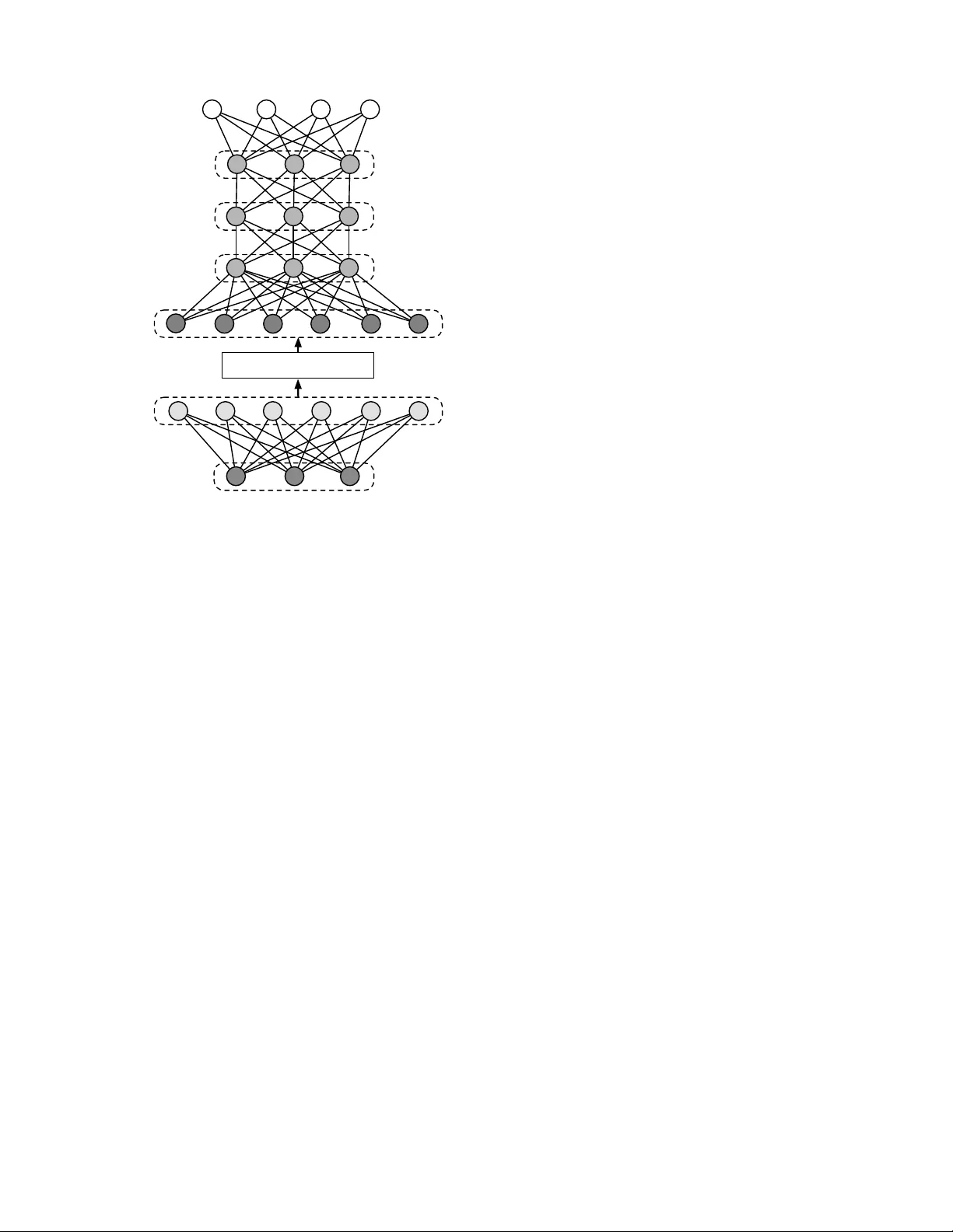
1 A Deep Bag-of-Features Model for Music Auto-T agging Juhan Nam, Member , IEEE, Jorge Herrera, and K yogu Lee, Senior Member , IEEE Abstract —Featur e learning and deep learning hav e drawn great attention in recent years as a way of transforming input data into more effective repr esentations using learning algo- rithms. Such interest has gr own in the area of music inf ormation retrie val (MIR) as well, particularly in music audio classification tasks such as auto-tagging. In this paper , we present a two- stage learning model to effecti vely predict multiple labels fr om music audio. The first stage learns to project local spectral patterns of an audio track onto a high-dimensional sparse space in an unsupervised manner and summarizes the audio track as a bag-of-featur es. The second stage successively performs the unsupervised learning on the bag-of-features in a layer-by-lay er manner to initialize a deep neural network and finally fine-tunes it with the tag labels. Through the experiment, we rigorously examine training choices and tuning parameters, and show that the model achieves high performance on Magnatagatune, a popularly used dataset in music auto-tagging. Index T erms —music information retriev al, feature learning, deep learning, bag-of-features, music auto-tagging, restricted Boltzmann machine (RBM), deep neural network (DNN). I . I N T R O D U C T I O N In the recent past music has become ubiquitous as digital data. The scale of music collections that are readily accessible via online music services surpassed thirty million tracks 1 . The type of music content has been also di versified as social media services allow people to easily share their own original music, cover songs or other media sources. These significant changes in the music industry have prompted new strategies for deliv ering music content, for example, searching a large volume of songs with different query methods (e.g., text, humming or audio example) or recommending a playlist based on user preferences. A successful approach to these needs is using meta data, for example, finding similar songs based on analysis by music experts or collaborativ e filtering based on user data. Howe ver , the analysis by experts is costly and limited, giv en the lar ge scale of av ailable music tracks. User data are intrinsically biased by the popularity of songs or artists. As a way of making up for these limitations of meta data, the audio content itself have been exploited, i.e., by training a system to predict high-le vel information from the music audio files. This content-based approach has been activ ely explored in the area of music information retrie val (MIR). They are usually formed as an audio classification task that predicts a single label giv en categories (e.g. genre or emotion) or multiple labels in various aspects of music. The J. Nam, J. Herrera and K. Lee are with Korea Advanced Institute of Science and T echnology , South Korea, Stanford University , CA, USA and Seoul National University , South K orea, respectiv ely . 1 http://press.spotify .com/us/information/, accessed in Jan 23, 2015 latter is often referred to as music annotation and retriev al, or simply called music auto-tagging . These audio classification tasks are generally implemented through two steps; feature extraction and supervised learning. While the supervised learning step is usually handled by commonly used classifiers such as Gaussian mixture model (GMM) and support vector machines (SVM), the feature extraction step has been extensiv ely studied based on domain knowledge. For e xample, Tzanetakis and Cook in their seminal work on music genre classification presented comprehensiv e signal processing techniques to extract audio features that represents timbral texture, rhythmic content and pitch content of music [1]. Specifically , they include lo w-level spectral summaries (e.g. centroid and roll-off), zero-crossings and mel- frequency cepstral coef ficients (MFCC), a wavelet transform- based beat histogram and pitch/chroma histogram. McKin- ney and Breebaart suggested perceptual audio features based on psychoacoustic models, including estimates of roughness, loudness and sharpness, and auditory filterbank temporal en- velopes [2]. Similarly , a number of audio features have been proposed with different choices of time-frequency represen- tations, psychoacoustic models and other signal processing techniques. Some of distinct audio features introduced in music classification include octav e-based spectral contrast [3], Daubechies wav elet coefficient histogram [4], and auditory temporal modulation [5]. A common aspect of these audio features is that they are hand-engineer ed . In other words, individual computation steps to extract the features from audio signals are manually de- signed based on signal processing and/or acoustic knowledge. Although this hand-engineering approach has been successful to some degree, it has limitations in that, by nature, it may require numerous trial-and-error in the process of fine-tuning the computation steps. For this reason, many of previous work rather combine existing audio features, for example, by concatenating MFCC and other spectral features [6], [7], [8]. Howe ver , they are usually heuristically chosen so that the combination can be redundant or still insufficient to explain music. Feature selection is a solution to finding an optimal combination but this is another challenge [9]. Recently there have been increasing interest in finding feature representations using data-driv en learning algorithms, as an alternati ve to the hand-engineering approach. Inspired by research in computational neuroscience [10], [11], the ma- chine learning community has dev eloped a variety of learning algorithms that discov er underlying structures of image or audio, and utilized them to represent features. This approach made it possible to overcome the limitations of the hand- 2 engineering approach by learning manifold patterns automat- ically from data. This learning-based approach is broadly referred to as featur e learning or r epresentation learning [12]. In particular , hierarchical representation learning based on deep neural network (DNN) or con volutional neural network (CNN), called deep learning , achie ved a remarkable series of successes in challenging machine recognition tasks, such as speech recognition [13] and image classification [14]. The ov erview and recent work are revie wed in [12], [15]. The learning-based approach has gained great interest in the MIR community as well. Le veraging adv ances in the machine learn- ing community , MIR researchers have in vestigated better ways of representing audio features and furthermore envisioned the approach as a general framew ork to build hierarchical music feature representations [16]. In particular, the ef forts hav e been made most activ ely for music genre classification or music auto-tagging. Using either unsupervised feature learning or deep learning, they have shown improved performance in the tasks. In this paper, we present a two-stage learning model as an extension of our previous work [17]. The first stage learns local features from multiple frames of audio spectra using sparse restricted Boltzmann machine (RBM) as before. Howe ver , we add an onset detection module to select temporally-aligned frames in training data. This is intended to decrease the v aria- tion in input space against random sampling. W e show that this helps improving performance giv en the same condition. The second stage continues the bottom-up unsupervised learning by applying RBMs (b ut without sparsity) to the bag-of-features in a layer-by-layer manner . W e use the RBM parameters to initialize a DNN and finally fine-tunes the network with the labels. W e sho w that this pretraining impro ves the performance as observed in image classification or speech recognition tasks. The remainder of this paper is organized as follo ws. In Section II, we overvie w related work. In Section III, we de- scribe the bag-of-features model. In Section IV, we introduce datasets, e valuation metrics and e xperiment settings. In Section V, we in vestigate the the ev aluation results and compare them to those of state-of-the-arts algorithms in music auto-tagging. Lastly , we conclude by providing a summary of the work in Section VI. I I . R E L AT ED W O R K In this section, we revi ew previous work that exploited feature learning and deep learning for music classification and music auto-tagging. They can be di vided into two groups, depending on whether the learning algorithm is unsupervised or supervised. One group in vestigated unsupervised feature learning based on sparse representations, for example, using K-means [18], [17], [19], [20], sparse coding [21], [22], [23], [17], [24] and restricted Boltzmann machine (RBM) [25], [17]. The majority of them focused on capturing local structures of music data ov er one or multiple audio frames to learn high-dimensional single-layer features. They summarized the locally learned features as a bag-of-features (also called a bag-of-frames , for example, in [26]) and fed them into a separate classifier . The advantage of this single-layer feature learning is that it is quite simple to learn a large-size of feature bases and they generally provide good performance [27]. In addition, it is easy to handle the v ariable length of audio tracks as they usually represent song-lev el features with summary statistics of the locally learned features (i.e. temporal pooling). Howe ver , this single- layer approach is limited to learning local features only . Some works worked on dual or multiple layers to capture segment- lev el features [28], [29]. Although they sho wed slight im- prov ement by combining the local and segment-lev el features, learning hierarchical structures of music in an unsupervised way is highly challenging. The second group used supervised learning that directly maps audio and labels via multi-layered neural networks. One approach was mapping single frames of spectrogram [30], [31], [32] or summarized spectrogram [33] to labels via DNNs, where some of them pretrain the networks with deep belief networks [30], [31], [33]. They used the hidden-unit activ ations of DNNs as local audio features. While this frame- lev el audio-to-label mapping is somewhat counter-intuitiv e, the supervised approach makes the learned features more discriminativ e for the given task, being directly comparable to hand-engineered features such as MFCC. The other approach in this group used CNNs where the con volution setting can take longer audio frames and the networks directly predict labels [34], [35], [36], [37]. CNNs has become the de-facto standard in image classification since the break-through in ImageNet challenge [14]. As such, the CNN-based approach has shown great performance in music auto-tagging [35], [37]. Howe ver , in order to achiev e high performance with CNNs, the model needs to be trained with a large dataset along with a huge number of parameters. Otherwise, CNNs is not necessarily better than the bag-of-features approach [19], [37]. Our approach is based on the bag-of-features in a single- layer unsupervised learning but e xtend it to a deep structure for song-lev el supervised learning. The idea behind this deep bag- of-features model is, while taking the simplicity and flexibility of the bag-of-features approach in unsupervised single-layer feature learning, improving the discriminative power using deep neural networks. Similar models were suggested using a different combination of algorithms, for example, K-means and multi-layer perceptrons (MLP) in [19], [20]. Ho wever , our proposed model performs unsupervised learning through all layers consistently using RBMs. I I I . L E A R N I N G M O D E L Figure 1 illustrates the ov erall data processing pipeline of our proposed model. In this section, we describe the individual processing blocks in details. A. Pr epr ocessing Musical signals are characterized well by note onsets and ensuing spectral patterns. W e perform se veral steps of front- end processing to help learning algorithms effecti vely capture the features. 3 Audio Tracks Automatic Gain Control Mel-Freq. Spectrogram Gaussian-Binary RBM w/Sparsity Amplitude Compression Multiple Frames PCA Whitening Onset Detection Function Max-pooling and Averaging Tags Preprocessing Local Feature Learning (Unsupervised) and Summarization Song-level Supervised Learning DNN ReLU-ReLU RBM Binary-ReLU RBM ReLU-ReLU RBM Fig. 1: The proposed deep bag-of-features model for music auto-tagging. The dotted lines indicate that the processing is conducted only in the training phase. 1) Automatic Gain Contr ol: Musical signals are highly dynamic in amplitude. Being inspired by the dynamic-range compression mechanism in human ears, we control the ampli- tude as a first step. W e adopt time-frequency automatic gain control which adjusts the lev els of sub-band signals separately [38]. Since we already showed the effecti veness in music auto- tagging [17], we use the automatic gain control as a default setting here. 2) Mel-fr equency Spectr ogram: W e use mel-frequency spectrogram as a primary input representation. The mel- frequency spectrogram is computed by mapping 513 linear frequency bins from FFT to 128 mel-frequency bins. This mapping reduces input dimensionality sufficiently so as to take multiple frames as input data while preserving distinct patterns of spectrogram well. 3) Amplitude Compr ession: The mel-frequency spectro- gram is additionally compressed with a log-scale function, log 10 (1 + C · x ) , where x is the mel-frequency spectrogram and C controls the degree of compression [39]. 4) Onset Detection Function: The local feature learning stage takes multiple frames as input data so that learning algorithms can capture spectro-temporal patterns, for exam- ple, sustaining or chirping harmonic overtones, or transient changes ov er time. W e already sho wed that using multiple frames for feature learning improves the performance in music auto-tagging [17]. W e further de velop this data selection scheme by considering where to take multiple frames on the time axis. In the previous work, we sampled multiple frames at random positions on the mel-frequency spectrogram without considering the characteristics of musical sounds. Therefore, giv en a single note, it could sample audio frames such that the note onset is located at arbitrary positions within the sampled frames or only sustain part of a note is taken. This may increase unnecessary variations or lose the chance of capturing important temporal dependency in the view of learning algorithm. In order to address this problem, we suggest sampling multiple frames based on the guidance of note onset. That is, we compute an onset detection function as a separate path and take a sample of multiple frames at the positions that the onset detection function has high values for a short segment. As illustrated in Figure 2, local spectral structures of musical sounds tend to be more distinctiv e when the onset strength is high. Sampled audio frames this way are likely to be aligned to each other with regard to notes, which may encourage learning algorithms to learn features more effecti vely . W e term this sampling scheme onset-based sampling and will ev aluate it in our experiment. The onset detection function is computed on a separate path by mapping the spectrogram on to 40 sub-bands and summing the half- wa ve rectified spectral flux ov er the sub-bands. B. Local F eatur e Learning and Summarization This stage first learns feature bases using the sampled data and learning algorithms. Then, it extracts the feature activ ations in a conv olutional manner for each audio track and summarizes them as a bag-of-features using max-pooling and av eraging. 1) PCA Whitening: PCA whitening is often used as a pre- processing step to remove pair-wise correlations (i.e. second- order dependence) or reduce the dimensionality before apply- ing algorithms that capture higher -order dependencies [40]. The PCA whitening matrix is computed by applying PCA to the sampled data and normalizing the output in the PCA space. Note that we locate PCA whitening as part of local feature learning in Figure 1 because the whitening matrix is actually “learned” by the sampled data. 2) Sparse Restricted Boltzmann Machine (RBM): Sparse RBM is the core algorithm that performs local feature learn- ing in the bag-of-features model. In our previous work, we compared K-means, sparse coding and sparse RBM in terms of performance of music auto-tagging [17]. Although there was not much difference, sparse RBM worked slightly better than others and the feed-forward computation for the hidden units in the RBM allows fast prediction in the testing phase. Thus, we focus only the sparse RBM here and more formally revie w the algorithm in the following paragraphs. Sparse RBM is a variation of RBM which is a bipartite undirected graphical model that consists of visible nodes v and hidden nodes h [41]. The visible nodes correspond to input vectors in a training set and the hidden nodes correspond to represented features. The basic form of RBM has binary units for both visible and hidden nodes, termed binary-binary RBM. The joint probability of v and h is defined by an energy function E ( v , h ) : 4 Mel−frequency Spectrogram Mel−frequency Bin 0.8 1 1.2 1.4 1.6 1.8 2 20 40 60 80 100 120 0.8 1 1.2 1.4 1.6 1.8 2 0 0.1 0.2 0.3 0.4 0.5 Onset Detection Function Seconds Onset Strength Fig. 2: Onset-based sampling. This data sampling scheme takes multiple frames at the positions that the onset strength is high. p ( v , h ) = e − E ( v , h ) Z (1) E ( v , h ) = −  b T v + c T h + v T Wh  (2) where b and c are bias terms, and W is a weight matrix. The normalization factor Z is called the partition function, which is obtained by summing all possible configurations of v and h . For real-v alued data such as spectrogram, Gaussian units are frequently used for the visible nodes. Then, the energy function in Equation 1 is modified to: E ( v , h ) = v T v −  b T v + c T h + v T Wh  (3) where the additional quadratic term, v T v is associated with cov ariance between input units assuming that the Gaussian units have unit v ariances. This form is called Gaussian-binary RBM [42]. The RBM has symmetric connections between the two layers but no connections within the hidden nodes or visible nodes. This conditional independence makes it easy to com- pute the conditional probability distributions, when nodes in either layer are observed: p ( h j = 1 | v ) = σ ( c j + X i W ij v i ) (4) p ( v i | h ) = N ( b i + X j W ij h j , 1) , (5) where σ ( x ) = 1 / (1 + exp( x )) is the logistic function and N ( x ) is the Gaussian distribution. These can be directly deriv ed from Equation 1 and 2. The model parameters of RBM are estimated by taking deriv ati ve of the log-likelihood with regard to each parameter and then updating them using gradient descent. The update rules for weight matrix and bias terms are obtained from Equation 1: W ij ← W ij +  ( h v i h j i data − h v i h j i model ) (6) b i ← b i +  ( h v i i data − h v i i model ) (7) c j ← c j +  ( h h j i data − h h j i model ) (8) where  is the learning rate and the angle brackets denote expectation with respect to the distributions from the training data and the model. While h v i h j i data can be easily obtained, exact computation of h v i h j i model is intractable. In practice, the learning rules in Equation 6 conv erges well only with a single iteration of block Gibbs sampling when it starts by setting the states of the visible units to the training data. This approximation is called the contrastive-diver gence [43]. This parameter estimation is solely based on maximum likelihood and so it is prone to overfitting to the training data. As a way of improving generalization to new data [44], the maximum likelihood estimation is penalized with additional terms called weight-decay . The typical choice is L 2 norm, which is half of the sum of the squared weights. T aking the deriv ati ve, the weight update rule in Equation 6 is modified to: W ij ← W ij +  ( h v i h j i data − h v i h j i model − µW ij ) (9) where µ is called weight-cost and controls the strength of the weight-decay . Sparse RBM is trained with an additional constraint on the update rules, which we call sparsity . W e impose the sparsity on hidden units of a Gaussian-binary RBM based on the technique in [41]. The idea is to add a penalty term that minimizes a deviation of the mean activ ation of hidden units from a target sparsity level. Instead of directly applying the gradient descent to that, they exploit the contrastive-di ver gence update rule and so simply added it to the update rule of bias term c j . This controls the hidden-unit activ ations as a shift term of the sigmoid function in Equation 4. As a result, the bias update rule in Equation 8 is modified to: c j ← c j +  ( h h j i data −h h j i model )+ λ X j ( ρ − 1 m ( m X k =1  h j | v k  )) 2 , (10) where { v 1 , ..., v m } is the training set, ρ determines the target sparsity of the hidden-unit activ ations and λ controls the strength. 3) Max-P ooling and A ver aging: Once we train a sparse RBM from the sampled data, we fix the learned parameters and extract the hidden-unit activ ations in a conv olutional manner for an audio track. Follo wing our previous work, we summarize the local features via max-pooling and av- eraging. Max-pooling has proved to be an effecti ve choice to summarize local features [34], [19]. It works as a form of temporal masking because it discards small acti vations around high peaks. W e further summarize the max-pooled feature acti vations with averaging. This produces a bag-of- features that represents a histogram of dominant local feature activ ations. C. Song-Level Learning This stage performs supervised learning to predict tags from the bag-of-features. Using a deep neural network (DNN), 5 Song-Level Bag-of-Features Max-Pooling / Averaging Hidden Layers Local Sparse Features PCA-whitened Mel-spectrogram Labels (T ags) Fig. 3: The architecture of bag-of-features model. The three fully connected layers are first pretrained with song-lev el bag- of-features data using stacked RBMs with ReLU and then fine- tuned with labels. we build a deep bag-of-featur es representation that maps the complex relations between the summarized acoustic features and semantic labels. W e configure the DNN to hav e up to three hidden layers and rectified linear units (ReLUs) for the nonlinear function as shown in Figure 3. The ReLUs hav e prov ed to be highly effecti ve in the DNN training when used with the dropout regularization [45], [46], [32], and also much faster than other nonlinear functions such as sigmoid in computation. W e first pretrain the DNN by a stack of RBMs and then fine-tune it using tag labels. The output layer works as multiple independent binary classifiers. Each output unit corresponds to a tag label and predicts whether the audio track is labeled with it or not. 1) Pr etraining: Pretraining is an unsupervised approach to better initialize the DNN [43]. Although recent advances have shown that pretraining is not necessary when the number of labeled training samples is suf ficient [14], [47], we conduct the pretraining to verify the necessity in our experiment setting. W e perform the pretraining by greedy layer-wise learning of RBMs with ReLUs to make learned parameters compatiable with the nonlinearity in the DNN. The ReLUs in the RBMs can be vie wed as the sum of an infinite number of binary units that share weights and have shifted versions of the same bias [48]. This can be approximated to a single unit with the max(0 , x ) nonlinearity . Furthermore, Gibbs sampling for the ReLUs during the training can be performed by taking samples from max(0 , x + N (0 , σ ( x ))) where N (0 , σ ( x )) is Gaussian noise with zero mean and v ariance σ ( x ) [48]. W e use the ReLU for both visible and hidden nodes of the stacked RBMs. Howe ver , for the bottom RBM that takes the bag-of-features as input data, we use binary units for visible nodes and ReLU for hidden notes to make them compatible with the scale of the bag-of-features. 2) F ine-tuning: After initializing the DNN with the weight and bias learned from the RBMs, we fine-tune them with tag labels using the error back-propagation. W e predict the output by adding the output layer (i.e. weight and bias) to the last hidden layer and taking the sigmoid function to define the error as cross-entropy between the prediction h θ,j ( x i ) and ground truth y ij ∈ { 0 , 1 } for bag-of-features i and tag j : J ( θ ) = X i X j y ij log( h θ,j ( x i )) + (1 − y ij )(1 − log( h θ,j ( x i ))) (11) W e update a set of parameters θ using AdaDelta. The method requires no manual tuning for the learning rate and is robust to noisy gradient information and v ariations in model architecture [49]. In addition, we use dropout, a po werful technique that improv es the generalization error of large neural networks by setting zeros to hidden and input layers randomly [50]. W e find AdaDelta and dropout essential to achiev e good performance. I V . E X P E R I M E N T S In the section, we introduce the dataset and ev aluation metrics used in o ur e xperiments. Also, we describe experiment settings for the proposed model. A. Datasets W e use the Magnatagatune dataset, which contains 29- second MP3 files with annotations collected from an online game [51]. The dataset is the MIREX 2009 version used in [34], [35]. It is split into 14660, 1629 and 6499 clips, respectiv ely for training, validation and test, follo wing the prior work. The clips are annotated with a set of 160 tags. B. Evaluation Metrics Follo wing the ev aluation metrics in [34], [35], we use the area under the receiv er operating characteristic curve over tag (A UC-T or shortly A UC), the same measure over clip (A UC- C) and top-K precision where K is 3, 6, 9, 12 and 15. C. Pr epr ocessing P arameters W e first con vert the MP3 files to the W A V format and resample them to 22.05kHz. W e then compute their spectro- gram with a 46ms Hann window and 50% overlap, on which the time-frequency automatic gain control using the technique in [38] is applied. This equalizes the spectrogram using spectral en velopes computed ov er 10 sub-bands. W e con vert the equalized spectrogram to mel-frequency spectrogram with 128 bins and finally compress the magnitude by fixing the strength C to 10. 6 Number of Frames 2 4 6 8 10 AUC 0.82 0.825 0.83 0.835 0.84 0.845 Random Sampling Number of Frames 2 4 6 8 10 AUC 0.82 0.825 0.83 0.835 0.84 0.845 Onset-based Sampling Fig. 4: Results for number of frames in the input spectral block and data sampling scheme. Each box contains the statistics of A UC for different sparsity and max-pooling sizes. D. Experiment Settings 1) Local F eatur e Learning and Summarization: The first step in this stage is to train PCA (for whitening) and sparse RBM. Each training sample is a spectral block comprised of multiple consecutiv e frames from the mel-frequency spec- trogram. W e gather training data (total 200,000 samples) by taking one spectral block every second at a random position or using the onset detection function. The number of frames in the spectral block varies from 2, 4, 6, 8 to 10 and we ev aluate them separately . W e obtain the PCA whitening matrix retaining 90% of the variance to reduce the dimensionality and then train the sparse RBM with a learning rate of 0.03, a hidden-layer size of 1024 and dif ferent v alues of target sparsity ρ from 0.007, 0.01, 0.02 to 0.03. Once we learn the PCA whitening matrix and RBM weight, we extract hidden-unit activ ations from an audio track in a con volutional manner and summarize them into a bag-of-features with max-pooling over segments with 0.25, 0.5, 1, 2 and 4 seconds. Since this stage creates a large number of possibilities in obtaining a bag-of-features, we reduce the number of adjustable parameters before proceeding with song-lev el su- pervised learning. Among others, we fix the number of frames in the spectral block and data sampling scheme, which are related to collecting the sample data. W e find a reasonable setting for them using a simple linear classifier that minimizes the same cross-entrop y in Equation 11 (i.e. logistic regression). 2) Song-Level Supervised Learning: W e first pretrain the DNN with RBMs and then fine-tune the networks. W e fix the hidden-layer size to 512 and adjust the number of hidden layers from 1 to 3 to verify the effect of larger networks. In training ReLU-ReLU RBMs, we set the learning rate to a small v alue (0.003) in order to av oid unstable dynamics in the weight updates [44]. W e also adjust the weight-cost in training RBMs from 0.001, 0.01 to 0.1, separately for each hidden layer . W e fine-tune the pretrained networks, using Deepmat, a Matlab library for deep learning 2 . This library includes an implementation of AdaDelta and dropout, and supports 2 https://github .com/kyunghyuncho/deepmat Number of Hidden Layers 1 2 3 AUC 0.87 0.872 0.874 0.876 0.878 0.88 0.882 0.884 0.886 0.888 0.89 Random Initialization Number of Hidden Layers 1 2 3 AUC 0.87 0.872 0.874 0.876 0.878 0.88 0.882 0.884 0.886 0.888 0.89 Pretraining Fig. 5: Results for dif ferent number of hidden layers. Each boxplot contains the statistics of A UC for different target sparsity and max-pooling sizes in the bag-of-features. GPU processing. In order to validate the proposed model, we compare it to DNNs with random initialization and also the same model but with ReLU units for the visible layer of the bottom RBM 3 V . R E S U L T S In this section, we examine training choices and tuning parameters in the experiments, and finally compare them to state-of-the-art results. A. Onset Detection Function and Number of F rames W e compare random sampling with onset-based sampling in the context of finding an optimal number of frames in local feature learning. In order to prevent the experiment from being too exhausting, we chose logistic regression as a classifier instead of the DNN. Figure 4 shows the ev aluation results. In random sampling, the A UC increases up to 6 frames and then slo wly decays. A similar trend is sho wn in onset- based sampling. Howe ver , the A UC saturates in a higher level, indicating that onset-based sampling is more effecti ve for the local feature learning. In the follo wing experiments, we fix the number of frames to 8 as it provides the highest A UC in terms of median. B. Pr etraining by ReLU RBMs Figure 5 shows the ev aluation results for dif ferent numbers of hidden layers when the DNN is randomly initialized or pretrained with ReLU RBMs. When the networks has a single hidden layer, there is no significant difference in A UC lev el. As the number of hidden layers increases in the DNN, howe ver , pretrained networks apparently outperform randomly initialized networks. This result is interesting, when recalling recent observations that pretraining is not necessary when the number of labeled training samples is suf ficient. Thus, the result may indicate that the size of labeled data is not 3 Our experiment code is available at https://github .com/juhannam/deepbof 7 Target Sparsity 0.007 0.01 0.02 0.03 AUC 0.88 0.881 0.882 0.883 0.884 0.885 0.886 0.887 0.888 0.889 0.89 Pooling Size [second] 0.25 0.5 1 2 4 AUC 0.88 0.881 0.882 0.883 0.884 0.885 0.886 0.887 0.888 0.889 0.89 Fig. 6: Results for dif ferent target sparsity and max-pooling sizes in the bag-of-features when we use a pretrained DNN with three hidden layers. large enough in our experiment. Ho wev er, we need to note that the auto-tagging task is formed as a multiple binary classification problem, which is different from choosing one label exclusiv ely , and furthermore the lev els of abstraction in the tag labels are not homogenous (e.g. including mood and instruments). In addition, there is some recent work that pretraining is still useful [46]. C. Sparsity and Max-pooling Figure 6 sho ws the ev aluation results for different target sparsity and max-pooling sizes in the bag-of-features when we use a pretrained DNN with three hidden layers. The best results are achieved when target sparsity is 0.02 and max- pooling size is 1 or 2 second. Compared to our previous work [17], the optimal target sparsity has not changed whereas the optimal max-pooling size is significantly reduced. Considering we used 30 second segments in the Maganatagatune dataset against the full audio tracks in the CAL500 datasets (typically 3-4 minute long), the optimal max-pooling size seems to be proportional to the length of audio tracks. D. W eight-Cost W e adjust weight-cost in training the RBM with three different values. Since this exponentially increases the number of networks to train as we stack up RBMs, a brute-force search for an optimal setting of weight-costs becomes very time-consuming. For example, when we have three hidden layers, we should fine-tune 27 different instances of pretrained networks. From our experiments, howe ver , we observed that the good results tend to be obtained when the bottom layer has a small weight-cost and upper layers have progressiv ely greater weight-costs. In order to validate the observation, we plot the statistics of A UC for a giv en weight-cost at each layer in Figure 7. For example, the left-most boxplot is computed from all combinations of weight-costs when the weight-cost in the first-layer RBM (L1) is fixed to 0.001 (this includes 9 combinations of weight-cost for three hidden layers. W e count them for all different target sparsity and max-pooling size). 0.001 0.01 0.1 0.001 0.01 0.1 0.001 0.01 0.1 AUC 0.878 0.88 0.882 0.884 0.886 0.888 L1 Weight-Cost L2 Weight-Cost L3 Weight-Cost Fig. 7: Results for a fixed weight-cost at each layer . Each boxplot contains the statistics of A UC for all weight-cost combinations in three hidden layers given the fixed weight- cost. For the first layer , the A UC goes up when the weight-cost is smaller . Howe ver , the trend becomes weaker through the second layer (L2) and goes opposite for the third layer (L3); the best A UC in median is obtained when the weight-cost is 0.1 for the third layer , even though the dif ference it slight. This result implies that it is better to encourage “maximum likelihood” for the first layer by having a small weight-cost and regulate it for upper layers by having progressiv ely greater weight-costs. This is plausible when considering the lev el of abstraction in the DNN that goes from acoustic feature summaries to semantic words. Based on this observ ation, we suggest a special condition for the weight-cost setting to reduce the number of pretraining instances. That is, we set the weight-cost to a small value (=0.001) for the first layer and an equal or increasing value for upper layers. Figure 8 compares the special condition denoted as “WC Inc” to the best result and fixed settings for all layers. “WC Inc” achiev es the best result in three out of four and it always outperforms the three fixed setting. This shows that, with the special condition for the weight-cost setting, we can sav e significant amount of training time while achieving high performance. E. Comparison with State-of-the-art Algorithms W e lastly compare our proposed model to previous state- of-the-art algorithms in music auto-tagging. Since we use the MIREX 2009 version of Magnatagatune dataset for which Hamel et. al. achiev ed the best performance [34], [35], we place their e valuation results only in T able I. They also used deep neural networks with a special preprocessing of mel- frequency spectrogram. Howe ver , our deep bag-of-features model outperforms them for all ev aluation metrics. V I . C O N C L U S I O N W e presented a deep bag-of-feature model for music auto- tagging. The model learns a large dictionary of local feature 8 Target Sparsity 0.007 0.01 0.02 0.03 AUC 0.88 0.882 0.884 0.886 0.888 0.89 WC=0.1 WC=0.01 WC=0.001 WC_Inc Best Fig. 8: Results for dif ferent settings of weight-costs in training RBMs. “Best” is the best result among all pretrained networks (27 instances). “WC=0.1”, “WC=0.01” and “WC=0.001” in- dicate when the weight-cost is fixed to the v alue for all hidden layers. “WC Inc” means the best result among instances where the weight-cost is 0.001 for the bottom layer and it is greater than or equal to the v alue for upper layers (this includes 6 combinations of weight-costs for three hidden layers). The max-pooling size is fixed to 1 second here. Methods A UC-T A UC-C P3 P6 P9 P12 P15 PMSC+PFC [34] 0.845 0.938 0.449 0.320 0.249 0.205 0.175 PSMC+MTSL [34] 0.861 0.943 0.467 0.327 0.255 0.211 0.181 Multi PMSCs [35] 0.870 0.949 0.481 0.339 0.263 0.216 0.184 Deep-BoF 0.888 0.956 0.511 0.358 0.275 0.225 0.190 T ABLE I: Performance comparison with Hamel et. al. ’ s results on the Magnatagatune dataset. bases on multiple frames selected by onset-based sampling and summarizes an audio track as a bag of learned audio features via max-pooling and averaging. Furthermore, it pre- trains and fine-tunes the DNN to predict the tags. The deep bag-of-feature model can be seen as a special case of deep con volutional neural networks as it has a con volution and pooling layer , where the local features are extracted and summarized, and has three fully connected layers. As future work, we will mov e on more general CNN models used in computer vision and train them with large-scale datasets. A C K N O W L E D G M E N T This work was supported by K orea Adv anced Institute of Science and T echnology (Project No. G04140049). R E F E R E N C E S [1] G. Tzanetakis and P . Cook, “Musical genre classification of audio signals, ” IEEE T ransaction on Speech and Audio Processing , 2002. [2] M. F . McKinney and J. Breebaart, “Features for audio and music classification, ” in Pr oceedings of the 4th International Conference on Music Information Retrieval (ISMIR) , 2003. [3] D.-N. Jiang, L. Lu, H.-J. Zhang, and J.-H. T ao, “Music type classification by spectral contrast feature, ” in Proceedings of International Confer ence on Multimedia Expo (ICME) , 2002. [4] T . Li, M. Ogihara, and Q. Li, “ A comparative study of content-based music genre classification, ” in Proceedings of the 26th international ACM SIGIR confer ence on Research and development in informaion r etrieval , 2003. [5] Y . Panagakis, C. K otropoulos, and G. R. Arce, “Non-negati ve multilinear principal component analysis of auditory temporal modulations for music genre classification, ” IEEE T ransaction on Audio, Speech and Language Processing , 2010. [6] J. Bergstra, N. Casagrande, D. Erhan, D. Eck, and B. Kegl, “ Aggregate features and adaboost for music classification, ” Machine Learning , 2006. [7] T . Bertin-Mahieux, D. Eck, F . Maillet, and P . Lamere, “ Autotagger: a model for predicting social tags from acoustic features on large music databases, ” in Journal of New Music Researc h , 2010. [8] K. K. C. J.-S. R. Jang and C. S. Iliopoulos, “Music genre classification via compressive sampling, ” in Pr oceedings of the 11th International Confer ence on Music Information Retrieval (ISMIR) , 2010. [9] C. N. Silla, A. K oerich, and C. Kaestner, “ A feature selection approach for automatic music genre classification, ” International Journal of Se- mantic Computing , 2008. [10] D. J. F . Bruno. A. Olshausen, “Emergence of simple-cellrecepti ve field properties by learning a sparse code for natural images, ” Nature , pp. 607–609, 1996. [11] M. S. Lewicki, “Ef ficient coding of natural sounds, ” Natur e Neur o- science , 2002. [12] Y . Bengio, A. Courville, and P . Vincent, “Representation learning:a revie w and new perspective, ” IEEE Tr ansaction on P attern Analysis and Machine Intelligennce , vol. 35, no. 8, pp. 1798–1828, 2013. [13] G. Hinton, L. Deng, D. Y u, G. Dahl, A. rahman Mohamed, N. Jaitly , A. Senior, V . V anhoucke, P . Nguyen, T . Sainath, and B. Kingsbury , “Deep neural networks for acoustic modeling in speech recognition, ” IEEE Signal Processing Magazine , 2012. [14] A. Krizhevsk y , I. Sutskev er, and G. E. Hinton, “Imagenet classfication with deep conv olutional neural networks, ” in Proceedings of the 25th Confer ence on Neural Information Pr ocessing Systems (NIPS) , 2012. [15] Y . Bengio, “Learning deep architectures for ai, ” F oundations and trends in Machine Learning , 2009. [16] E. J. Humphrey , J. P . Bello, and Y . LeCun, “Moving beyond feature design: Deep architectures and automatic feature learning in music informatics, ” in Pr oceedings of the 13th International Conference on Music Information Retrieval (ISMIR) , 2012. [17] J. Nam, J. Herrera, M. Slaney , and J. O. Smith, “Learning sparse feature representations for music annotation and retrieval, ” in Proceedings of the 13th International Conference on Music Information Retrieval (ISMIR) , 2012. [18] J. W ¨ ulfing and M. Riedmiller , “Unsupervised learning of local features for music classification, ” in Proceedings of the 13th International Confer ence on Music Information Retrieval (ISMIR) , 2012. [19] S. Dieleman and B. Schrauwen, “Multiscale approaches to music audio feature learning, ” in Pr oceedings of the 14th International Conference on Music Information Retrieval (ISMIR) , 2013. [20] A. van den Oord, S. Dieleman, and B. Schrauwen, “Transfer learning by supervised pre-training for audio-based music classification, ” in Pr oceedings of the 15th International Conference on Music Information Retrieval (ISMIR) , 2014. [21] R. Grosse, R. Raina, H. Kwong, and A. Y . Ng, “Shift-inv ariant sparse coding for audio classification, ” in Proceedings of the Conference on Uncertainty in AI , 2007. [22] P .-A. Manzagol, T . Bertin-Mahieux, and D. Eck, “On the use of sparse time-relativ e auditory codes for music, ” in Proceedings of the 9th International Confer ence on Music Information Retrieval (ISMIR) , 2008. [23] M. Henaff, K. Jarrett, K. Kavukcuoglu, and Y . LeCun, “Unsupervised learning of sparse features for scalable audio classification, ” in Pro- ceedings of the 12th International Conference on Music Information Retrieval (ISMIR) , 2011. [24] Y . V aizman, B. McFee, and G. Lanckriet, “Codebook based audio feature representation for music information retrieval, ” IEEE Tr ansactions on Acoustics, Speech and Signal Processing , 2014. [25] J. Schl ¨ uter and C. Osendorfer, “Music Similarity Estimation with the Mean-Cov ariance Restricted Boltzmann Machine, ” in Proceedings of the 10th International Conference on Machine Learning and Applications , 2011. [26] L. Su, C.-C. M. Y eh, J.-Y . Liu, J.-C. W ang, and Y .-H. Y ang, “ A systematic e valuation of the bag-of-frames representation for music information retrieval, ” IEEE T ransactions on Acoustics, Speech and Signal Pr ocessing , 2014. 9 [27] A. Coates, H. Lee, and A. Ng, “ An analysis of single-layer networks in unsupervised feature learning, ” Journal of Machine Learning Resear ch , 2011. [28] H. Lee, Y . Lar gman, P . Pham, and A. Y . Ng, “Unsupervised feature learn- ing for audio classification using conv olutional deep belief networks, ” in Advances in Neural Information Processing Systems 22 , 2009, pp. 1096–1104. [29] C.-C. M. Y eh, L. Su, and Y .-H. Y ang, “Dual-layer bag-of-frames model for music genre classification, ” in Proceedings of the 37th International Confer ence on Acoustics, Speech, and Signal Processing (ICASSP) , 2013. [30] P . Hamel and D. Eck, “Learning features from music audio with deep belief networks, ” in In Pr oceedings of the 11th International Conference on Music Information Retrieval (ISMIR) , 2010. [31] E. M. Schmidt and Y . E. Kim, “Learning emotion-based acoustic features with deep belief networks, ” in Proceedings of the 2011 IEEE W orkshop on Applications of Signal Pr ocessing to Audio and Acoustics (W ASP AA) , 2011. [32] S. Sigtia and S. Dixon, “Improved music feature learning with deep neural networks, ” in Pr oceedings of the 38th International Confer ence on Acoustics, Speech, and Signal Pr ocessing (ICASSP) , 2014. [33] E. M. Schmidt, J. Scott, and Y . E. Kim, “Feature learning in dynamic en vironments:modeling the acoustic structure of musical emotion, ” in Pr oceedings of the 13th International Conference on Music Information Retrieval (ISMIR) , 2012. [34] P . Hamel, S. Lemieux, Y . Bengio, and D. Eck, “T emporal pooling and multiscale learning for automatic annotation and ranking of music audio, ” in Proceedings of the 12th International Conference on Music Information Retrieval (ISMIR) , 2011. [35] P . Hamel, Y . Bengio, and D. Eck, “Building musically-relev ant audio features through multiple timescale representations, ” in Pr oceedings of the 13th International Conference on Music Information Retrieval (ISMIR) , 2012. [36] A. van den Oord, S. Dieleman, and B. Schrauwen, “Deep content- based music recommendation, ” in Proceedings of the 27th Conference on Neural Information Processing Systems (NIPS) , 2013. [37] S. Dieleman and B. Schrauwen, “End-to-end learning for music audio, ” in Proceedings of the 38th International Conference on Acoustics, Speech, and Signal Pr ocessing (ICASSP) , 2014. [38] D. Ellis, “Time-frequency automatic gain control, ” web resource, av ail- able, http://labrosa.ee.columbia.edu/matlab/tf agc/, 2010. [39] M. M ¨ uller , D. Ellis, A. Klapuri, and G. Richard, “Signal processing for music analysis, ” IEEE Journal on Selected T opics in Signal Processing , 2011. [40] A. Hyv ¨ arinen, J. Hurri, and P . O. Hoyer , Natural Image Statistics . Springer-V erlag, 2009. [41] H. Lee, C. Ekanadham, and A. Y . Ng, “Sparse deep belief net model for visual area V2, ” in Advances in Neural Information Pr ocessing Systems 20 , 2008, pp. 873–880. [42] Y . Bengio, P . Lamblin, D. Popovici, and H. Larochelle, “Greedy layer- wise training of deep networks, ” Advances in Neural Information Pr ocessing Systems 19 , 2007. [43] G. E. Hinton, S. Osindero, and Y .-W . T eh, “ A fast learning algorithm for deep belief nets, ” Neural computation , vol. 18, pp. 1527–1554, 2006. [44] G. E. Hinton, “ A practical guide to training restricted boltzmann machines, ” UTML T ec hnical Report , vol. 2010-003, 2010. [45] M. D. Zeiler, M. Ranzato, R. Monga, M. Mao, K. Y ang, Q. V . Le, P . Nguyen, A. Senior , V . V anhouck e, J. Dean, and G. E. Hinton, “On rectified linear units for speech processing, ” in Pr oceedings of the IEEE International Conference on Acoustics, Speech and Signal Processing (ICASSP) , 2013. [46] G. Dahl, T . N. Sainath, and G. Hinton, “Improving deep neural networks for lvcsr using rectified linear units and dropout, ” in Proceedings of the IEEE International Conference on Acoustics, Speech and Signal Pr ocessing (ICASSP) , 2013. [47] D. Y u and L. Deng, Automatic Speech Recognition-A Deep Learning Appr oach . Springer , 2015. [48] V . Nair and G. Hinton, “Rectified linear units improve restricted boltz- mann machines, ” in Proceedings of the 27th International Confer ence on Machine Learning (ICML) , 2010. [49] M. D. Zeiler, “ Adadelta: An adaptiv e learning rate method, ” in arXiv:1212.5701v1 , 2012. [50] N. Srivasta va, G. Hinton, A. Krizhevsk y , I. Sutskever , and R. Salakhut- dinov , “Dropout: A simple way to pre vent neural networks from over- fitting, ” Journal of Machine Learning Resear ch , 2014. [51] E. Law and L. V . Ahn, “Input-agreement: a new mechanism for collecting data using human computation games, ” in Proc. Intl. Conf. on Human factors in computing systems, CHI. ACM , 2009.