Unitary Evolution Recurrent Neural Networks

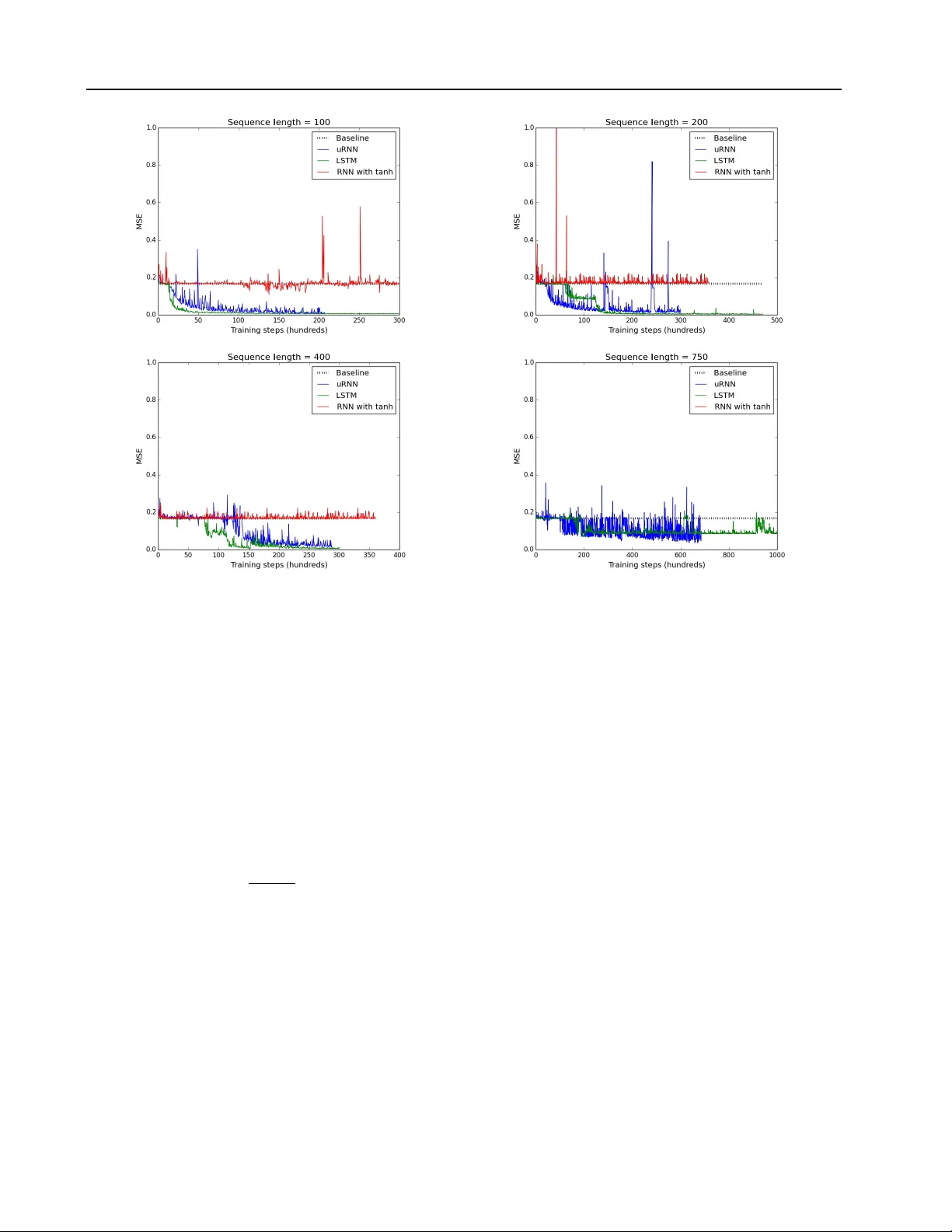
Unitary Evolution Recurr ent Neural Networks Martin Arjovsky ∗ M A R J OV S K Y @ D C . U B A . A R Amar Shah ∗ A S 7 9 3 @ C A M . AC . U K Y oshua Bengio Univ ersidad de Buenos Aires, Univ ersity of Cambridge, Univ ersit ´ e de Montr ´ eal. Y oshua Bengio is a CIF AR Senior Fellow . ∗ Indicates first authors. Ordering determined by coin flip. Abstract Recurrent neural networks (RNNs) are notori- ously dif ficult to train. When the eigen values of the hidden to hidden weight matrix de viate from absolute value 1, optimization becomes dif- ficult due to the well studied issue of vanish- ing and exploding gradients, especially when try- ing to learn long-term dependencies. T o circum- vent this problem, we propose a ne w architecture that learns a unitary weight matrix, with eigen- values of absolute v alue exactly 1. The chal- lenge we address is that of parametrizing uni- tary matrices in a w ay that does not require e x- pensiv e computations (such as eigendecomposi- tion) after each weight update. W e construct an expressi ve unitary weight matrix by composing sev eral structured matrices that act as building blocks with parameters to be learned. Optimiza- tion with this parameterization becomes feasible only when considering hidden states in the com- plex domain. W e demonstrate the potential of this architecture by achieving state of the art re- sults in sev eral hard tasks inv olving very long- term dependencies. 1. Introduction Deep Neural Networks hav e shown remarkably good per- formance on a wide range of complex data problems in- cluding speech recognition ( Hinton et al. , 2012 ), image recognition ( Krizhevsky et al. , 2012 ) and natural language processing ( Collobert et al. , 2011 ). Ho wever , training very deep models remains a difficult task. The main issue sur- rounding the training of deep networks is the vanishing and exploding gradients problems introduced by Hochre- Pr oceedings of the 33 rd International Conference on Machine Learning , New Y ork, NY , USA, 2016. JMLR: W&CP v olume 48. Copyright 2016 by the author(s). iter ( 1991 ) and sho wn by Bengio et al. ( 1994 ) to be nec- essarily arising when trying to learn to reliably store bits of information in any parametrized dynamical system. If gradients propagated back through a network vanish, the credit assignment role of backpropagation is lost, as infor- mation about small changes in states in the far past has no influence on future states. If gradients e xplode, gradient- based optimization algorithms struggle to trav erse down a cost surface, because gradient-based optimization assumes small changes in parameters yield small changes in the ob- jectiv e function. As the number of time steps considered in the sequence of states gro ws, the shrinking or expanding effects associated with the state-to-state transformation at individual time steps can grow exponentially , yielding re- spectiv ely vanishing or exploding gradients. See Pascanu et al. ( 2010 ) for a revie w . Although the long-term dependencies problem appears intractable in the absolute ( Bengio et al. , 1994 ) for parametrized dynamical systems, several heuristics hav e recently been found to help reduce its ef fect, such as the use of self-loops and gating units in the LSTM ( Hochre- iter & Schmidhuber , 1997 ) and GR U ( Cho et al. , 2014 ) re- current architectures. Recent w ork also supports the idea of using orthogonal weight matrices to assist optimization ( Saxe et al. , 2014 ; Le et al. , 2015 ). In this paper , we explore the use of orthogonal and unitary matrices in recurrent neural netw orks. W e start in Section 2 by showing a no vel bound on the propagated gradients in recurrent nets when the recurrent matrix is orthogonal. Sec- tion 3 discusses the difficulties of parameterizing real val- ued orthogonal matrices and how they can be alle viated by moving to the comple x domain. W e discuss a nov el approach to constructing expressi ve unitary matrices as the composition of simple unitary ma- trices which require at most O ( n log n ) computation and O ( n ) memory , when the state vector has dimension n . These are unlike general matrices, which require O ( n 2 ) computation and memory . Complex v alued representations Unitary Evolution Recurrent Neural Networks hav e been considered for neural networks in the past, but with limited success and adoption ( Hirose , 2003 ; Zimmer- mann et al. , 2011 ). W e hope our findings will change this. Whilst our model uses complex valued matrices and pa- rameters, all implementation and optimization is possible with real numbers and has been done in Theano ( Bergstra et al. , 2010 ). This along with other implementation details are discussed in Section 4 , and the code used for the e xper- iments is av ailable online. The potential of the developed model for learning long term dependencies with relatively few parameters is explored in Section 5 . W e find that the proposed architecture generally outperforms LSTMs and previous approaches based on orthogonal initialization. 2. Orthogonal W eights and Bounding the Long-T erm Gradient A matrix, W , is orthogonal if W > W = WW > = I . Orthogonal matrices hav e the property that they preserve norm (i.e. k W h k 2 = k h k 2 ) and hence repeated iterati ve multiplication of a vector by an orthogonal matrix leaves the norm of the vector unchanged. Let h T and h t be the hidden unit vectors for hidden layers T and t of a neural network with T hidden layers and T  t . If C is the objective we are trying to minimize, then the vanishing and exploding gradient problems refer to the decay or growth of ∂ C ∂ h t as the number of layers, T , grows. Let σ be a pointwise nonlinearity function, and z t +1 = W t h t + V t x t +1 h t +1 = σ ( z t +1 ) (1) then by the chain rule ∂ C ∂ h t = ∂ C ∂ h T ∂ h T ∂ h t = ∂ C ∂ h T T − 1 Y k = t ∂ h k +1 ∂ h k = ∂ C ∂ h T T − 1 Y k = t D k +1 W T k (2) where D k +1 = diag ( σ 0 ( z k +1 )) is the Jacobian matrix of the pointwise nonlinearity . In the following we define the norm of a matrix to refer to the spectral radius norm (or operator 2-norm) and the norm of a v ector to mean L 2 -norm. By definition of the oper- ator norms, for any matrices A , B and vector v we have k A v k ≤ k A k k v k and k AB k ≤ k A k k B k . If the weight matrices W k are norm preserving (i.e. orthogonal), then we pro ve     ∂ C ∂ h t     =      ∂ C ∂ h T T − 1 Y k = t D k +1 W T k      ≤     ∂ C ∂ h T     T − 1 Y k = t   D k +1 W T k   =     ∂ C ∂ h T     T − 1 Y k = t k D k +1 k . (3) Since D k is diagonal, k D k k = max j =1 ,...,n | σ 0 ( z ( j ) k ) | , with z ( j ) k the j -th pre-activ ation of the k -th hidden layer . If the absolute value of the deriv ativ e σ 0 can take some value τ > 1 , then this bound is useless, since k ∂ C ∂ h t k ≤    ∂ C ∂ h T    τ T − t which gro ws exponentially in T . W e there- fore cannot effecti vely bound ∂ C ∂ h t for deep networks, re- sulting potentially in exploding gradients. In the case | σ 0 | < τ < 1 , equation 3 proves that that ∂ C ∂ h t tends to 0 exponentially fast as T grows, resulting in guar- anteed vanishing gradients. This argument makes the rec- tified linear unit (ReLU) nonlinearity an attractive choice ( Glorot et al. , 2011 ; Nair & Hinton , 2010 ). Unless all the activ ations are killed at one layer, the maximum entry of D k is 1, resulting in k D k k = 1 for all layers k . W ith ReLU nonlinearities, we thus hav e     ∂ C ∂ h t     ≤     ∂ C ∂ h T     T − 1 Y k = t k D k +1 k =     ∂ C ∂ h T     . (4) Most notably , this result holds for a network of arbitrary depth and renders engineering tricks like gradient clipping unnecessary ( Pascanu et al. , 2010 ). T o the best of our knowledge, this analysis is a novel con- tribution and the first time a neural network architecture has been mathematically prov en to av oid exploding gradients. 3. Unitary Evolution RNNs Unitary matrices generalize orthogonal matrices to the complex domain. A complex valued, norm preserving ma- trix, U , is called a unitary matrix and is such that U ∗ U = UU ∗ = I , where U ∗ is the conjugate transpose of U . Di- rectly parametrizing the set of unitary matrices in such a way that gradient-based optimization can be applied is not straightforward because a gradient step will typically yield a matrix that is not unitary , and projecting on the set of uni- tary matrices (e.g., by performing an eigendecomposition) generally costs O ( n 3 ) computation when U is n × n . The most important feature of unitary and orthogonal ma- trices for our purpose is that they ha ve eigen values λ j with Unitary Evolution Recurrent Neural Networks absolute value 1. The follo wing lemma, prov ed in ( Hof f- man & K unze , 1971 ), may shed light on a method which can be used to efficiently span a large set of unitary matri- ces. Lemma 1. A complex squar e matrix W is unitary if and only if it has an eigendecomposition of the form W = VD V ∗ , where ∗ denotes the conjugate tr anspose. Here , V , D ∈ C n × n ar e complex matrices, wher e V is unitary , and D is a diagonal such that | D j,j | = 1 . Furthermor e, W is a r eal ortho gonal matrix if and only if for e very eigen- value D j,j = λ j with eigen vector v j , there is also a com- plex conjugate eigen value λ k = λ j with corr esponding eigen vector v k = v j . Writing λ j = e iw j with w j ∈ R , a nai ve method to learn a unitary matrix would be to fix a basis of eigenv ectors V ∈ C n × n and set W = VD V ∗ , (5) where D is a diagonal such that D j,j = λ j . Lemma 1 informs us how to construct a real orthogonal matrix, W . W e must (i) ensure the columns of V come in complex conjugate pairs, v k = v j , and (ii) tie weights w k = − w j in order to achiev e e iw j = e iw k . Most neu- ral network objecti ve functions are differentiable with re- spect to the weight matrices, and consequently w j may be learned by gradient descent. Unfortunately the above approach has undesirable proper- ties. Fixing V and learning w requires O  n 2  memory , which is unacceptable gi ven that the number of learned pa- rameters is O ( n ) . Further note that calculating V u for an arbitrary vector u requires O ( n 2 ) computation. Setting V to the identity would satisfy the conditions of the lemma, whilst reducing memory and computation requirements to O ( n ) , howe ver , W would remain diagonal, and ha ve poor representation capacity . W e propose an alternative strategy to parameterize unitary matrices. Since the product of unitary matrices is itself a unitary matrix, we compose sev eral simple, parameteric, unitary matrices to construct a single, expressi ve unitary matrix. The four unitary building blocks considered are • D , a diagonal matrix with D j,j = e iw j , with parame- ters w j ∈ R , • R = I − 2 v v ∗ k v k 2 , a reflection matrix in the complex vector v ∈ C n , • Π , a fixed random index permutation matrix, and • F and F − 1 , the F ourier and in verse Fourier trans- forms. Appealingly , D , R and Π all permit O ( n ) storage and O ( n ) computation for matrix vector products. F and F − 1 require no storage and O ( n log n ) matrix vector multiplica- tion using the Fast Fourier T ransform algorithm. A major advantage of composing unitary matrices of the form listed abov e, is that the number of parameters, memory and com- putational cost increase almost linearly in the size of the hidden layer . W ith such a weight matrix, immensely large hidden layers are feasible to train, whilst being impossible in traditional neural networks. W ith this in mind, in this work we choose to consider recur- rent neural networks with unitary hidden to hidden weight matrices. Our claim is that the ability to hav e large hidden layers where hidden states norms are preserved provides a powerful tool for modeling long term dependencies in sequence data. ( Bengio et al. , 1994 ) suggest that having a lar ge memory may be crucial for solving dif ficult tasks with long ranging dependencies: the smaller the state di- mension, the more information necessarily has to be elimi- nated when mapping a long sequence to a fixed-dimension state. W e call any RNN architecture which uses a unitary hidden to hidden matrix a unitary e volution RNN (uRNN). After experimenting with se veral structures, we settled on the fol- lowing composition W = D 3 R 2 F − 1 D 2 ΠR 1 F D 1 . (6) Whilst each but the permutation matrix is complex, we parameterize and represent them with real numbers for im- plementation purposes. When the final cost is real and dif- ferentiable, we may perform gradient descent optimization to learn the parameters. ( Y ang et al. , 2015 ) construct a real valued, non-orthogonal matrix using a similar parameter - ization with the motiv ation of parameter reduction by an order of magnitude on an industrial sized network. This combined with earlier work ( Le et al. , 2010 ) suggests that it is possible to create highly e xpressiv e matrices by compos- ing simple matrices with few parameters. In the following section, we explain details on how to implement our model and illustrate how we bypass the potential difficulties of working in the complex domain. 4. Architectur e details In this section, we describe the nonlinearity we used, how we incorporate real v alued inputs with complex valued hid- den units and map from complex hidden states to real out- puts. 4.1. Complex hidden units Our implementation represents all complex numbers us- ing real v alues in terms of their real and imaginary parts. Unitary Evolution Recurrent Neural Networks Under this framew ork, we sidestep the lack of support for complex numbers by most deep learning frameworks. Consider multiplying the comple x weight matrix W = A + i B by the complex hidden vector h = x + iy , where A , B , x, y are real. It is tri vially true that W h = ( A x − B y ) + i ( A y + B x ) . When we represent v ∈ C n as  Re ( v ) > , I m ( v ) >  > ∈ R 2 n , we compute complex matrix vector products with real numbers as follo ws  Re ( W h ) I m ( W h )  =  A − B B A   Re ( h ) I m ( h )  . (7) More generally , let f : C n → C n be any comple x func- tion and z = x + iy any complex v ector . W e may write f ( z ) = α ( x, y ) + iβ ( x, y ) where α, β : R n → R n . This allows us to implement ev erything using real valued oper- ations, compatible with any any deep learning frame work with automatic differentiation such as Theano. 4.2. Input to Hidden, Nonlinearity , Hidden to Output As is the case with most recurrent networks, our uRNN fol- lows the same hidden to hidden mapping as equation 1 with V t = V and W t = W . Denote the size of the complex valued hidden states as n h . The input to hidden matrix is complex v alued, V ∈ C n h × n in . W e learn the initial hidden state h 0 ∈ C n h as a parameter of the model. Choosing an appropriate nonlinearity is not trivial in the complex domain. As discussed in the introduction, using a ReLU is a natural choice in combination with a norm pre- serving weight matrix. W e first experimented with placing separate ReLU activ ations on the real and imaginary parts of the hidden states. Howe ver , we found that such a non- linearity usually performed poorly . Our intuition is that ap- plying separate ReLU nonlinearities to the real and imagi- nary parts brutally impacts the phase of a complex number , making it difficult to learn structure. W e speculate that maintaining the phase of hidden states may be important for storing information across a lar ge number of time steps, and our experiments supported this claim. A variation of the ReLU that we name modReLU , is what we finally chose. It is a pointwise nonlinearity , σ modReLU ( z ) : C → C , which af fects only the absolute value of a comple x number , defined as σ modReLU ( z ) =  ( | z | + b ) z | z | if | z | + b ≥ 0 0 if | z | + b < 0 (8) where b ∈ R is a bias parameter of the nonlinearity . For a n h dimensional hidden space we learn n h nonlinearity bias parameters, one per dimension. Note that the modReLU is similar to the ReLU in spirit, in fact more concretely σ modReLU ( z ) = σ ReLU ( | z | + b ) z | z | . T o map hidden states to output, we define a matrix U ∈ R n o × 2 n h , where n o is the output dimension. W e calculate a linear output as o t = U  Re ( h t ) I m ( h t )  + b o , (9) where b o ∈ R n o is the output bias. The linear output is real valued ( o t ∈ R n o ) and can be used for prediction and loss function calculation akin to typical neural networks (e.g. it may be passed through a softmax which is used for cross entropy calculation for classification tasks). 4.3. Initialization Due to the stability of the norm preserving operations of our network, we found that performance was not very sen- sitiv e to initialization of parameters. For full disclosure and reproducibility , we explain our initialization strategy for each parameter below . • W e initialize V and U (the input and out- put matrices) as in ( Glorot & Bengio , 2010 ), with weights sampled independently from uniforms, U h − √ 6 √ n in + n out , √ 6 √ n in + n out i . • The biases, b and b o are initialized to 0. This implies that at initialization, the network is linear with unitary weights, which seems to help early optimization ( Saxe et al. , 2014 ). • The reflection vectors for R 1 and R 2 are initialized coordinate-wise from a uniform U [ − 1 , 1] . Note that the reflection matrices are inv ariant to scalar multipli- cation of the parameter vector , hence the width of the uniform initialization is unimportant. • The diagonal weights for D 1 , D 2 and D 3 are sam- pled from a uniform, U [ − π , π ] . This ensures that the diagonal entries D j,j are sampled uniformly ov er the complex unit circle. • W e initialize h 0 with a uniform, U h − q 3 2 n h , q 3 2 n h i , which results in E  k h 0 k 2  = 1 . Since the norm of the hidden units are roughly preserved through unitary ev olution and inputs are typically whitened to hav e norm 1, we hav e hidden states, inputs and linear out- puts of the same order of magnitude, which seems to help optimization. 5. Experiments In this section we explore the performance of our uRNN in relation to (a) RNN with tanh activ ations, (b) IRNN ( Le et al. , 2015 ), that is an RNN with ReLU activ ations and with the recurrent weight matrix initialized to the identity , Unitary Evolution Recurrent Neural Networks Figure 1. Results of the copying memory problem for time lags of 100 , 200 , 300 , 500 . The LSTM is able to beat the baseline only for 100 times steps. Conv ersely the uRNN is able to completely solv e each time length in very fe w training iterations, without getting stuck at the baseline. and (c) LSTM ( Hochreiter & Schmidhuber , 1997 ) mod- els. W e show that the uRNN shines quantitativ ely when it comes to modeling long term dependencies and exhibits qualitativ ely dif ferent learning properties to the other mod- els. W e chose a handful of tasks to e valuate the performance of the various models. The tasks were especially created to be be pathologically hard, and hav e been used as bench- marks for testing the ability of a model to capture long-term memory ( Hochreiter & Schmidhuber , 1997 ; Le et al. , 2015 ; Grav es et al. , 2014 ; Martens & Sutske ver , 2011 ) Of the handful of optimization algorithms we tried on the various models, RMSProp ( Tieleman & Hinton , 2012 ) lead to fastest con vergence and is what we stuck to for all ex- periments here on in. Ho wev er , we found the IRNN to be particularly unstable; it only ran without blowing up with incredibly low learning rates and gradient clipping. Since the performance was so poor relativ e to other models we compare against, we do not show IRNN curves in the fig- ures. In each experiment we use a learning rate of 10 − 3 and a decay rate of 0 . 9 . For the LSTM and RNN models, we had to clip gradients at 1 to av oid exploding gradients. Gradient clipping was unnecessary for the uRNN. 5.1. Copying memory problem Recurrent networks ha ve been kno wn to hav e trouble re- membering information about inputs seen many time steps previously ( Bengio et al. , 1994 ; Pascanu et al. , 2010 ). W e therefore want to test the uRNN’ s ability to recall exactly data seen a long time ago. Follo wing a similar setup to ( Hochreiter & Schmidhuber , 1997 ), we outline the copy memory task. Consider 10 cate- gories, { a i } 9 i =0 . The input takes the form of a T + 20 length vector of categories, where we test over a range of values of T . The first 10 entries are sampled uniformly , indepen- dently and with replacement from { a i } 7 i =0 , and represent the sequence which will need to be remembered. The next T − 1 entries are set to a 8 , which can be thought of as the ’blank’ cate gory . The ne xt single entry is a 9 , which rep- resents a delimiter , which should indicate to the algorithm that it is no w required to reproduce the initial 10 categories in the output. The remaining 10 entries are set to a 8 . The required output sequence consists of T + 10 repeated en- tries of a 8 , followed by the first 10 categories of the input Unitary Evolution Recurrent Neural Networks Figure 2. Results of the adding problem for T = 100 , 200 , 400 , 750 . The RNN with tanh is not able to beat the baseline for any time length. The LSTM and the uRNN sho w similar performance across time lengths, consistently beating the baseline. sequence in exactly the same order . The goal is to mini- mize the average cross entropy of cate gory predictions at each time step of the sequence. The task amounts to hav- ing to remember a categorical sequence of length 10, for T time steps. A simple baseline can be established by considering an optimal strategy when no memory is a v ailable, which we deem the memoryless strategy . The memoryless strategy would be to predict a 8 for T + 10 entries and then predict each of the final 10 categories from the set { a i } 7 i =0 inde- pendently and uniformly at random. The categorical cross entropy of this strategy is 10 log(8) T +20 . W e ran experiments where the RNN with tanh acti vations, IRNN, LSTM and uRNN had hidden layers of size 80, 80, 40 and 128 respectively . This equates to roughly 6500 pa- rameters per model. In Figure 1 , we see that aside from the simplest case, both the RNN with tanh and more surpris- ingly the LSTMs get almost exactly the same cost as the memoryless strategy . This beha viour is consistent with the results of ( Grav es et al. , 2014 ), in which poor performance is reported for the LSTM for a very similar long term mem- ory problem. The uRNN consistently achie ves perfect performance in relativ ely few iterations, ev en when ha ving to recall se- quences after 500 time steps. What is remarkable is that the uRNN does not get stuck at the baseline at all, whilst the LSTM and RNN do. This behaviour suggests that the representations learned by the uRNN hav e qualitatively dif- ferent properties from both the LSTM and classical RNNs. 5.2. Adding Problem W e closely follo w the adding problem defined in ( Hochre- iter & Schmidhuber , 1997 ) to explain the task at hand. Each input consists of two sequences of length T . The first se- quence, which we denote x , consists of numbers sampled uniformly at random U [0 , 1] . The second sequence is an in- dicator sequence consisting of exactly two entries of 1 and remaining entries 0. The first 1 entry is located uniformly at random in the first half of the sequence, whilst the sec- ond 1 entry is located uniformly at random in the second half. The output is the sum of the tw o entries of the first se- quence, corresponding to where the 1 entries are located in the second sequence. A nai ve strategy of predicting 1 as the output regardless of the input sequence gives an e xpected mean squared error of 0 . 167 , the variance of the sum of two independent uniform distributions. This is our baseline to beat. Unitary Evolution Recurrent Neural Networks Figure 3. Results on pixel by pixel MNIST classification tasks. The uRNN is able to conv erge in a fraction of the iterations that the LSTM requires. The LSTM performs better on MNIST classification, but the uRNN outperforms on the more complicated task of permuted pixels. W e chose to use 128 hidden units for the RNN with tanh, IRNN and LSTM and 512 for the uRNN. This equates to roughly 16K parameters for the RNN with tanh and IRNN, 60K for the LSTM and almost 9K for the uRNN. All mod- els were trained using batch sizes of 20 and 50 with the best results being reported. Our results are shown in Figure 2 . The LSTM and uRNN models are able to con vincingly beat the baseline up to T = 400 time steps. Both models do well when T = 750 , but the mean squared error does not reach close to 0 . The uRNN achieves lo wer test error , but it’ s curve is more noisy . Despite having vastly more param- eters, we monitored the LSTM performance to ensure no ov erfitting. The RNN with tanh and IRNN were not able to beat the baseline for any number of time steps. ( Le et al. , 2015 ) re- port that their RNN solv e the problem for T = 150 and the IRNN for T = 300 , b ut they require over a million itera- tions before they start learning. Neither of the two mod- els came close to either the uRNN or the LSTM in perfor- mance. The stark difference in our findings are best ex- plained by our use of RMSprop with significantly higher learning rates ( 10 − 3 as opposed to 10 − 8 ) than ( Le et al. , 2015 ) use for SGD with momentum. 5.3. Pixel-by-pixel MNIST In this task, suggested by ( Le et al. , 2015 ), algorithms are fed pixels of MNIST ( LeCun et al. , 1998 ) sequentially and required to output a class label at the end. W e consider two tasks: one where pixels are read in order (from left to right, bottom to top) and one where the pix els are all randomly permuted using the same randomly generated permutation matrix. The same model architectures as for the adding problem were used for this task, except we now use a soft- max for category classification. W e ran the optimization algorithms until con ver gence of the mean categorical cross entropy on test data, and plot test accuracy in Figure 3 . Both the uRNN and LSTM perform applaudably well here. On the correct unpermuted MNIST pixels, the LSTM per- forms better , achie ving 98.2 % test accurracy v ersus 95.1% for the uRNN. Howe ver , when we permute the ordering of the pixels, the uRNN dominates with 91.4% of accuracy in contrast to the 88% of the LSTM, despite having less than a quarter of the parameters. This result is state of the art on this task, beating the IRNN ( Le et al. , 2015 ), which reaches close to 82% after 1 million training iterations. Notice that uRNN reaches con vergence in less than 20 thousand itera- tions, while it takes the LSTM from 5 to 10 times as many to finish learning. Permuting the pixels of MNIST images creates many longer term dependencies across pixels than in the origi- nal pix el ordering, where a lot of structure is local. This makes it necessary for a network to learn and remember more complicated dependencies across v arying time scales. The results suggest that the uRNN is better able to deal with such structure o ver the data, where the LSTM is better suited to more local sequence structure tasks. 5.4. Exploratory experiments Norms of hidden state gradients. As discussed in Sec- tion 2 , key to being able to learn long term dependencies is in controlling ∂ C ∂ h t . With this in mind, we explored ho w each model propagated gradients, by examining    ∂ C ∂ h t    as a function of t . Gradient norms were computed at the be- Unitary Evolution Recurrent Neural Networks Figure 4. From left to right. Norms of the gradients with respect to hidden states i.e.    ∂ C ∂ h t    at (i) beginning of training, (ii) after 100 iterations. (iii) Norms of the hidden states and (iv) L 2 distance between hidden states and final hidden state. The gradient norms of uRNNs do not decay as fast as for other models as training progresses. uRNN hidden state norms stay much more consistent over time than the LSTM. LSTM hidden states stay almost the same after a number of time steps, suggesting that it is not able to use new input information. ginning of training and again after 100 iterations of training on the adding problem. The curves are plotted in Figure 4 . It is clear that at first, the uRNN propagates gradients per- fectly , while each other model has exponentially vanishing gradients. After 100 iterations of training, each model ex- periences v anishing gradients, but the uRNN is best able to propagate information, having much less decay . Hidden state saturation. W e claim that typical recurrent architectures saturate, in the sense that after they acquire some information, it becomes much more difficult to ac- quire further information pertaining to longer dependen- cies. W e took the uRNN and LSTM models trained on the adding problem with T = 200 , and computed a for- ward pass with newly generated data for the adding prob- lem with T = 1000 . In order to sho w saturation effects, we plot the norms of the hidden states and the L 2 distance between each state and the last in Figure 4 . In our e xperiments, it is clear that the uRNN does not suffer as much as other models do. Notice that whilst the norms of hidden states in the uRNN gro w very steadily o ver time, in the LSTM they gro w very fast, and then stay constant after about 500 time steps. This beha viour may suggest that the LSTM hidden states saturate in their ability to incorporate new information, which is vital for modeling long com- plicated sequences. It is interesting to see that the LSTM hidden state at t = 500 , is close to that of t = 1000 , whilst this is far from the case in the uRNN. Again, this suggests that the LSTM’ s capacity to use new information to alter its hidden state sev erly de grades with sequence length. The uRNN does not suffer from this dif ficulty nearly as badly . A clear example of this phenomenon was observed in the adding problem with T = 750 . W e found that the Pearson correlation between the LSTM output prediction and the first of the two uniform samples (whose sum is the tar get output) was ρ = 0 . 991 . This suggests that the LSTM learnt to simply find and store the first sample, as it was unable to incorporate any more information by the time it reached the second, due to saturation of the hidden states. 6. Discussion There are a plethora of further ideas that may be explored from our findings, both with re gards to learning representa- tion and ef ficient implementation. For e xample, one hurdle of modeling long sequences with recurrent networks is the requirement of storing all hidden state values for the pur - pose of gradient backpropagation. This can be prohibiti ve, since GPU memory is typically a limiting factor of neural network optimization. Ho wev er , since our weight matrix is unitary , its in verse is its conjugate transpose, which is just as easy to operate with. If further we were to use an in vert- ible nonlinearity function, we would no longer need to store hidden states, since they can be recomputed in the back- ward pass. This could have potentially huge implications, as we would be able to reduce memory usage by an order of T , the number of time steps. This w ould make having immensely large hidden layers possible, perhaps enabling vast memory representations. In this paper we demonstrate state of the art performance on hard problems requiring long term reasoning and mem- ory . These results are based on a novel parameterization of unitary matrices which permit efficient matrix compu- tations and parameter optimization. Whilst complex do- main modeling has been widely succesful in the signal pro- cessing community (e.g. Fourier transforms, wa velets), we hav e yet to exploit the power of complex valued represen- tation in the deep learning community . Our hope is that this work will be a step forw ard in this direction. W e moti- vate the idea of unitary e volution as a novel way to mitigate the problems of vanishing and exploding gradients. Empir- ical evidence suggests that our uRNN is better able to pass gradient information through long sequences and does not suffer from saturating hidden states as much as LSTMs, typical RNNs, or RNNs initialized with the identity weight matrix (IRNNs). Unitary Evolution Recurrent Neural Networks Acknowledgments : W e thank the dev elopers of Theano ( Bergstra et al. , 2010 ) for their great work. W e thank NSERC, Compute Canada, Canada Research Chairs and CIF AR for their support. W e would also like to thank C ¸ aglar Gulc ¸ ehre, David Krueger , Soroush Mehri, Marcin Moczulski, Mohammad Pezeshki and Saizheng Zhang for helpful discussions, comments and code sharing. References Bengio, Y oshua, Simard, Patrice, and Frasconi, Paolo. Learning long-term dependencies with gradient descent is difficult. IEE T ransactions on Neural Networks , 5, 1994. Bergstra, James, Breuleux, Oli vier , Bastien, Fr ´ ed ´ eric, Lamblin, Pascal, Pascanu, Razvan, Desjardins, Guil- laume, Turian, Joseph, W arde-Farley , David, and Ben- gio, Y oshua. Theano: a CPU and GPU math expression compiler . Pr oceedings of the Python for Scientific Com- puting Confer ence (SciPy) , 2010. Cho, Kyunghyun, v an Merri ¨ enboer , Bart, Bahdanau, Dzmitry , and Bengio, Y oshua. On the properties of neu- ral machine translation: Encoder–Decoder approaches. In Eighth W orkshop on Syntax, Semantics and Structur e in Statistical T ranslation , October 2014. Collobert, Ronan, W eston, Jason, Bottou, L ´ eon, Karlen, Michael, Kavukcuoglu, Koray , and Kuksa, Pa vel. Natu- ral language processing (almost) from scratch. Journal of Machine Learning Resear ch , 12:2493–2537, 2011. Glorot, Xavier and Bengio, Y oshua. Understanding the difficulty of training deep feedforward neural networks. International Conference on Artificial Intelligence and Statistics (AIST ATS) , 2010. Glorot, Xavier , Bordes, Antoine, and Bengio, Y oshua. Deep sparse rectifier neural networks. International Confer ence on Artificial Intelligence and Statistics (AIS- T ATS) , 2011. Grav es, Alex, W ayne, Greg, and Danihelka, Ivo. Neural turing machines. arXiv pr eprint arXiv:1410.5401 , 2014. Hinton, Geof frey , Deng, Li, Y u, Dong, Dahl, George, Mo- hamed, Abdel-rahman, Jaitly , Na vdeep, Senior , Andre w , V anhoucke, V incent, Nguyen, P atrick, Sainath, T ara, and Kingsbury , Brian. Deep neural networks for acoustic modeling in speech recognition. Signal Processing Mag- azine , 2012. Hirose, Akira. Complex-valued neural networks: theories and applications , v olume 5. W orld Scientific Publishing Company Incorporated, 2003. Hochreiter , S. Untersuchungen zu dynamischen neu- ronalen Netzen. Diploma thesis, T .U. M ¨ unich, 1991. Hochreiter , Sepp and Schmidhuber , J ¨ urgen. Long short- term memory . Neur al Computation , 8(9):1735–1780, 1997. Hoffman, K enneth and Kunze, Ray . Linear Algebra . Pear - son, second edition, 1971. Krizhevsk y , Alex, Sutske ver , Ilya, and Hinton, Geoffre y E. Imagenet classification with deep conv olutional neu- ral networks. Neural Information Pr ocessing Systems , 2012. Le, Quoc, Sarl ´ os, T am ´ as, and Smola, Alex. Fastfood - ap- proximating kernel expansions in loglinear time. Inter - national Confer ence on Machine Learning , 2010. Le, Quoc V ., Na vdeep, Jaitly , and Hinton, Geof frey E. A simple way to initialize recurrent netw orks of rectified linear units. arXiv pr eprint arXiv:1504.00941 , 2015. LeCun, Y ann, Bottou, L ´ eon, Bengio, Y oshua, and Haffner , Patrick. Gradient-based learning applied to document recognition. Pr oceedings of the IEEE , 1998. Martens, James and Sutskev er , Ilya. Learning recurrent neural networks with hessian-free optimization. Inter - national Confer ence on Machine Learning , 2011. Nair , V inod and Hinton, Geoffre y E. Rectified linear units improv e restricted boltzmann machines. International Confer ence on Machine Learning , 2010. Pascanu, Razvan, Mikolov , T omas, and Bengio, Y oshua. On the dif ficulty of training recurrent neural networks. International Confer ence on Machine Learning , 2010. Saxe, Andrew M., McLelland, James L., and Ganguli, Surya. Exact solutions to the nonlinear dynamics of learning in deep linear neural networks. International Confer ence in Learning Repr esentations , 2014. T ieleman, Tijmen and Hinton, Geoffre y . Lecture 6.5- rmsprop: Divide the gradient by a running av erage of its recent magnitude. Coursera: Neural Networks for Machine Learning , 2012. Y ang, Zichao, Moczulski, Marcin, Denil, Misha, de Fre- itas, Nando, Smola, Alex, Song, Le, and W ang, Ziyu. Deep fried con vnets. International Confer ence on Com- puter V ision (ICCV) , 2015. Zimmermann, Hans-Georg, Minin, Alexey , and Kusherbae va, V ictoria. Comparison of the com- plex valued and real valued neural networks trained with gradient descent and random search algorithms. In ESANN , 2011.