Increasing the Interpretability of Recurrent Neural Networks Using Hidden Markov Models

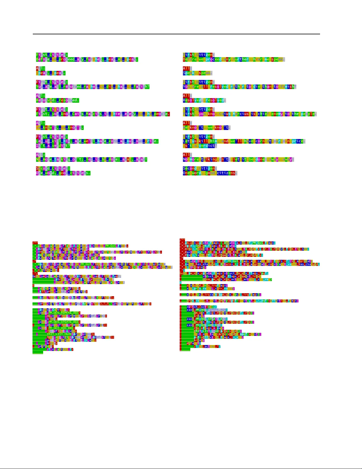
Incr easing the Interpr etability of Recurr ent Neural Netw orks Using Hidden Marko v Models V iktoriya Krakovna V K R A KO V NA @ FA S . H A RV A R D . E D U Department of Statistics, Harvard Uni v ersity Finale Doshi-V elez FI NA L E @ S E A S . H A RV A R D . E D U Department of Computer Science, Harvard Uni v ersity Abstract As deep neural networks continue to re v olu- tionize various application domains, there is in- creasing interest in making these powerful mod- els more understandable and interpretable, and narrowing down the causes of good and bad predictions. W e focus on recurrent neural net- works (RNNs), state of the art models in speech recognition and translation. Our approach to increasing interpretability is by combining an RNN with a hidden Markov model (HMM), a simpler and more transparent model. W e explore various combinations of RNNs and HMMs: an HMM trained on LSTM states; a hybrid model where an HMM is trained first, then a small LSTM is gi v en HMM state distributions and trained to fill in gaps in the HMM’ s performance; and a jointly trained hybrid model. W e find that the LSTM and HMM learn complementary information about the features in the text. 1. Introduction Follo wing the recent progress in deep learning, researchers and practitioners of machine learning are recognizing the importance of understanding and interpreting what goes on inside these black box models. Recurrent neural net- works hav e recently re volutionized speech recognition and translation, and these powerful models could be very useful in other applications in v olving sequential data. Howe v er , adoption has been slow in applications such as health care, where practitioners are reluctant to let an opaque expert system make crucial decisions. If we can make the inner workings of RNNs more interpretable, more applications can benefit from their power . 2016 ICML W orkshop on Human Interpr etability in Mac hine Learning (WHI 2016) , New Y ork, NY , USA. Copyright by the author(s). There are sev eral aspects of what makes a model or algorithm understandable to humans. One aspect is model complexity or parsimony . Another aspect is the ability to trace back from a prediction or model component to particularly influential features in the data ( R ¨ uping , 2006 ) ( Kim et al. , 2015 ). This could be useful for understanding mistakes made by neural networks, which hav e human- lev el performance most of the time, b ut can perform very poorly on seemingly easy cases. For instance, conv olu- tional networks can misclassify adversarial examples with very high confidence ( Nguyen et al. , 2015 ), and made headlines in 2015 when the image tagging algorithm in Google Photos mislabeled African Americans as gorillas. It’ s reasonable to expect recurrent networks to fail in similar ways as well. It would thus be useful to have more visibility into where these sorts of errors come from, i.e. which groups of features contrib ute to such flawed predictions. Sev eral promising approaches to interpreting RNNs have been dev eloped recently . Che et al. ( 2015 ) have approached this by using gradient boosting trees to predict LSTM output probabilities and explain which features played a part in the prediction. They do not model the internal structure of the LSTM, but instead approximate the entire architecture as a black box. Karpathy et al. ( 2016 ) showed that in LSTM language models, around 10% of the memory state dimensions can be interpreted with the nak ed eye by color-coding the text data with the state values; some of them track quotes, brackets and other clearly identifiable aspects of the text. Building on these results, we tak e a somewhat more systematic approach to looking for inter- pretable hidden state dimensions, by using decision trees to predict individual hidden state dimensions (Figure 2 ). W e visualize the ov erall dynamics of the hidden states by coloring the training data with the k-means clusters on the state vectors (Figures 3b , 3d ). W e explore se veral methods for building interpretable mod- els by combining LSTMs and HMMs. The existing body 46 Are RNNs and HMMs Mor e Interpretable When Combined? of literature mostly focuses on methods that specifically train the RNN to predict HMM states ( Bourlard & Mor gan , 1994 ) or posteriors ( Maas et al. , 2012 ), referred to as hybrid or tandem methods respectiv ely . W e first in vestig ate an approach that does not require the RNN to be modified in order to make it understandable, as the interpretation happens after the f act. Here, we model the big picture of the state changes in the LSTM, by extracting the hidden states and approximating them with a continuous emission hidden Markov model (HMM). W e then tak e the rev erse approach where the HMM state probabilities are added to the output layer of the LSTM (see Figure 1 ). The LSTM model can then make use of the information from the HMM, and fill in the gaps when the HMM is not performing well, resulting in an LSTM with a smaller num- ber of hidden state dimensions that could be interpreted individually (Figures 3 , 4 ). 2. Methods W e compare a hybrid HMM-LSTM approach with a con- tinuous emission HMM (trained on the hidden states of a 2-layer LSTM), and a discrete emission HMM (trained directly on data). 2.1. LSTM models W e use a character -le vel LSTM with 1 layer and no dropout, based on the Element-Research library . W e train the LSTM for 10 epochs, starting with a learning rate of 1, where the learning rate is halved whenev er exp( − l t ) > exp( − l t − 1 ) + 1 , where l t is the log likelihood score at epoch t . The L 2 -norm of the parameter gradient vector is clipped at a threshold of 5. 2.2. Hidden Markov models The HMM training procedure is as follows: Initialization of HMM hidden states: (Discrete HMM) Random multinomial dra w for each time step (i.i.d. across time steps). (Continuous HMM) K-means clusters fit on LSTM states, to speed up con v ergence relative to random initialization. At each iteration: 1. Sample states using Forw ard Filtering Backwards Sampling algorithm (FFBS, Rao & T eh ( 2013 )). 2. Sample transition parameters from a Multinomial- Dirichlet posterior . Let n ij be the number of tran- sitions from state i to state j . Then the posterior Figure 1: Hybrid HMM-LSTM algorithm. distribution of the i -th ro w of transition matrix T (corresponding to transitions from state i ) is: T i ∼ Mult ( n ij | T i ) Dir ( T i | α ) where α is the Dirichlet hyperparameter . 3. (Continuous HMM) Sample multi variate normal emission parameters from Normal-In v erse-W ishart posterior for state i : µ i , Σ i ∼ N ( y | µ i , Σ i ) N ( µ i | 0 , Σ i ) IW (Σ i ) (Discrete HMM) Sample the emission parameters from a Multinomial-Dirichlet posterior . Evaluation: W e e v aluate the methods on ho w well the y predict the ne xt observation in the v alidation set. For the HMM models, we do a forward pass on the validation set (no backward pass unlike the full FFBS), and compute the HMM state distribution vector p t for each time step t . Then we compute the predicti v e likelihood for the next observation as follows: P ( y t +1 | p t ) = n X x t =1 n X x t +1 =1 p tx t · T x t ,x t +1 · P ( y t +1 | x t +1 ) where n is the number of hidden states in the HMM. 47 Are RNNs and HMMs Mor e Interpretable When Combined? Figure 2: Decision tree predicting an individual hidden state dimension of the hybrid algorithm based on the preceding characters on the Linux data. The hidden state dimensions of the 10-state hybrid mostly track comment characters. 2.3. Hybrid models Our main hybrid model is put together sequentially , as shown in Figure 1 . W e first run the discrete HMM on the data, outputting the hidden state distrib utions obtained by the HMM’ s forward pass, and then add this information to the architecture in parallel with a 1-layer LSTM. The linear layer between the LSTM and the prediction layer is augmented with an e xtra column for each HMM state. The LSTM component of this architecture can be smaller than a standalone LSTM, since it only needs to fill in the gaps in the HMM’ s predictions. The HMM is written in Python, and the rest of the architecture is in T orch. W e also build a joint hybrid model, where the LSTM and HMM are simultaneously trained in T orch. W e imple- mented an HMM T orch module, optimized using stochastic gradient descent rather than FFBS. Similarly to the sequen- tial hybrid model, we concatenate the LSTM outputs with the HMM state probabilities. 3. Experiments W e test the models on sev eral text data sets on the character lev el: the Penn Tree Bank (5M characters), and two data sets used by Karpathy et al. ( 2016 ), Tin y Shakespeare (1M characters) and Linux Kernel (5M characters). W e chose k = 20 for the continuous HMM based on a PCA analysis of the LSTM states, as the first 20 components captured almost all the variance. T able 1 shows the predictive log likelihood of the next text character for each method. On all text data sets, the hybrid algorithm performs a bit better than the standalone LSTM with the same LSTM state dimension. This ef fect gets smaller as we increase the LSTM size and the HMM makes less difference to the prediction (though it can still mak e a difference in terms of interpretability). The hybrid algorithm with 20 HMM states does better than the one with 10 HMM states. The joint hybrid algorithm outperforms the sequential hybrid on Shak espeare data, but does worse on PTB and Linux data, which suggests that the joint hybrid is more helpful for smaller data sets. The joint hybrid is an order of magnitude slower than the sequential hybrid, as the SGD-based HMM is slo wer to train than the FFBS-based HMM. W e interpret the HMM and LSTM states in the hybrid algorithm with 10 LSTM state dimensions and 10 HMM states in Figures 3 and 4 , showing which features are identified by the HMM and LSTM components. In Figures 3a and 3c , we color-code the training data with the 10 HMM states. In Figures 3b and 3d , we apply k-means clustering to the LSTM state vectors, and color-code the training data with the clusters. The HMM and LSTM states pick up on spaces, indentation, and special characters in the data (such as comment symbols in Linux data). W e see some examples where the HMM and LSTM complement each other , such as learning different things about spaces and comments on Linux data, or punctuation on the Shake- speare data. In Figure 2 , we see that some indi vidual LSTM hidden state dimensions identify similar features, such as comment symbols in the Linux data. 48 Are RNNs and HMMs Mor e Interpretable When Combined? (a) Hybrid HMM component: colors correspond to 10 HMM states. Blue cluster identifies spaces. Green cluster (with white font) identifies punctuation and ends of words. Purple cluster picks up on some vo wels. (b) Hybrid LSTM component: colors correspond to 10 k-means clusters on hidden state vectors. Y ellow cluster (with red font) identifies spaces. Gre y cluster identifies punctuation (e xcept commas). Purple cluster finds some ’y’ and ’o’ letters. Figure 3: V isualizing HMM and LSTM states on Shakespeare data for the hybrid with 10 LSTM state dimensions and 10 HMM states. The HMM and LSTM components learn some complementary features in the text: while both learn to identify spaces, the LSTM does not completely identify punctuation or pick up on v o wels, which the HMM has already done. (c) Hybrid HMM component: colors correspond to 10 HMM states. Distinguishes comments and indentation spaces (green with yellow font) from other spaces (purple). Red cluster (with yello w font) identifies punctuation and brackets. Green cluster (yellow font) also finds capitalized variable names. (d) Hybrid LSTM component: colors correspond to 10 k-means clusters on hidden state vectors. Distinguishes comments, spaces at beginnings of lines, and spaces between words (red with white font) from indentation spaces (green with yellow font). Opening brackets are red (yello w font) and closing brackets are green (white font). Figure 4: V isualizing HMM and LSTM states on Linux data for the hybrid with 10 LSTM state dimensions and 10 HMM states. The HMM and LSTM components learn some complementary features in the te xt related to spaces and comments. 49 Are RNNs and HMMs Mor e Interpretable When Combined? T able 1: Predictive loglikelihood comparison on the text data sets (sorted by validation set performance). Data Method Parameters LSTM dims HMM states V alidation T raining Shakespeare Continuous HMM 1300 20 -2.74 -2.75 Discrete HMM 650 10 -2.69 -2.68 Discrete HMM 1300 20 -2.5 -2.49 LSTM 865 5 -2.41 -2.35 Hybrid 1515 5 10 -2.3 -2.26 Hybrid 2165 5 20 -2.26 -2.18 LSTM 2130 10 -2.23 -2.12 Joint hybrid 1515 5 10 -2.21 -2.18 Hybrid 2780 10 10 -2.19 -2.08 Hybrid 3430 10 20 -2.16 -2.04 Hybrid 4445 15 10 -2.13 -1.95 Joint hybrid 3430 10 10 -2.12 -2.07 LSTM 3795 15 -2.1 -1.95 Hybrid 5095 15 20 -2.07 -1.92 Hybrid 6510 20 10 -2.05 -1.87 Joint hybrid 4445 15 10 -2.03 -1.97 LSTM 5860 20 -2.03 -1.83 Hybrid 7160 20 20 -2.02 -1.85 Joint hybrid 7160 20 10 -1.97 -1.88 Linux Kernel Discrete HMM 1000 10 -2.76 -2.7 Discrete HMM 2000 20 -2.55 -2.5 LSTM 1215 5 -2.54 -2.48 Joint hybrid 2215 5 10 -2.35 -2.26 Hybrid 2215 5 10 -2.33 -2.26 Hybrid 3215 5 20 -2.25 -2.16 Joint hybrid 4830 10 10 -2.18 -2.08 LSTM 2830 10 -2.17 -2.07 Hybrid 3830 10 10 -2.14 -2.05 Hybrid 4830 10 20 -2.07 -1.97 LSTM 4845 15 -2.03 -1.9 Joint hybrid 5845 15 10 -2.00 -1.88 Hybrid 5845 15 10 -1.96 -1.84 Hybrid 6845 15 20 -1.96 -1.83 Joint hybrid 9260 20 10 -1.90 -1.76 LSTM 7260 20 -1.88 -1.73 Hybrid 8260 20 10 -1.87 -1.73 Hybrid 9260 20 20 -1.85 -1.71 Penn T ree Bank Continuous HMM 1000 100 20 -2.58 -2.58 Discrete HMM 500 10 -2.43 -2.43 Discrete HMM 1000 20 -2.28 -2.28 LSTM 715 5 -2.22 -2.22 Hybrid 1215 5 10 -2.14 -2.15 Joint hybrid 1215 5 10 -2.08 -2.08 Hybrid 1715 5 20 -2.06 -2.07 LSTM 1830 10 -1.99 -1.99 Hybrid 2330 10 10 -1.94 -1.95 Joint hybrid 2830 10 10 -1.94 -1.95 Hybrid 2830 10 20 -1.93 -1.94 LSTM 3345 15 -1.82 -1.83 Hybrid 3845 15 10 -1.81 -1.82 Hybrid 4345 15 20 -1.8 -1.81 Joint hybrid 6260 20 10 -1.73 -1.74 LSTM 5260 20 -1.72 -1.73 Hybrid 5760 20 10 -1.72 -1.72 Hybrid 6260 20 20 -1.71 -1.71 4. Conclusion and future work Hybrid HMM-RNN approaches combine the interpretabil- ity of HMMs with the predictiv e po wer of RNNs. Some- times, a small hybrid model can perform better than a standalone LSTM of the same size. W e use visualizations to show how the LSTM and HMM components of the hy- brid algorithm complement each other in terms of features learned in the data. References Bourlard, Herve and Morgan, Nelson. Connectionist speech r ecognition: a hybrid approac h , volume 247 of Kluwer international series in engineering and computer science . Kluwer Academic Publishers, Boston, 1994. Che, Zhengping, Purushotham, Sanjay , and Liu, Y an. Distilling Kno wledge from Deep Networks with Applications to Healthcare Domain. Neural Information Pr ocessing Systems W orkshop on Machine Learning for Healthcar e (MLHC) , 2015. Karpathy , Andrej, Johnson, Justin, and Li, Fei-Fei. V isualizing and Understanding Recurrent Networks. International Conference for Learning Representations W orkshop T rack , 2016. Kim, Been, Shah, Julie A., and Doshi-V elez, Finale. Mind the gap: A generativ e approach to interpretable feature selection and extraction. In Cortes, Corinna, Lawrence, Neil D., Lee, Daniel D., Sugiyama, Masashi, and Garnett, Roman (eds.), Neural Information Pr ocessing Systems (NIPS) , pp. 2260–2268, 2015. Maas, A., Le, Q., O’Neil, T ., V in yals, O., Nguyen, P ., and Ng, A. Recurrent Neural Networks for Noise Reduction in Robust ASR. In Pr oceedings of INTERSPEECH , 2012. Nguyen, Anh Mai, Y osinski, Jason, and Clune, Jeff. Deep neural networks are easily fooled: High confidence predictions for unrecognizable images. In IEEE Conference on Computer V ision and P attern Recognition, CVPR 2015, Boston, MA, USA, J une 7-12, 2015 , pp. 427–436, 2015. Rao, V inayak and T eh, Y ee Whye. Fast MCMC sampling for Markov jump processes and extensions. J ournal of Machine Learning Resear c h , 14:3207–3232, 2013. R ¨ uping, Stefan. Learning interpr etable models . PhD thesis, Dortmund Univ ersity of T echnology , 2006. 50