Bibliographic Analysis on Research Publications using Authors, Categorical Labels and the Citation Network

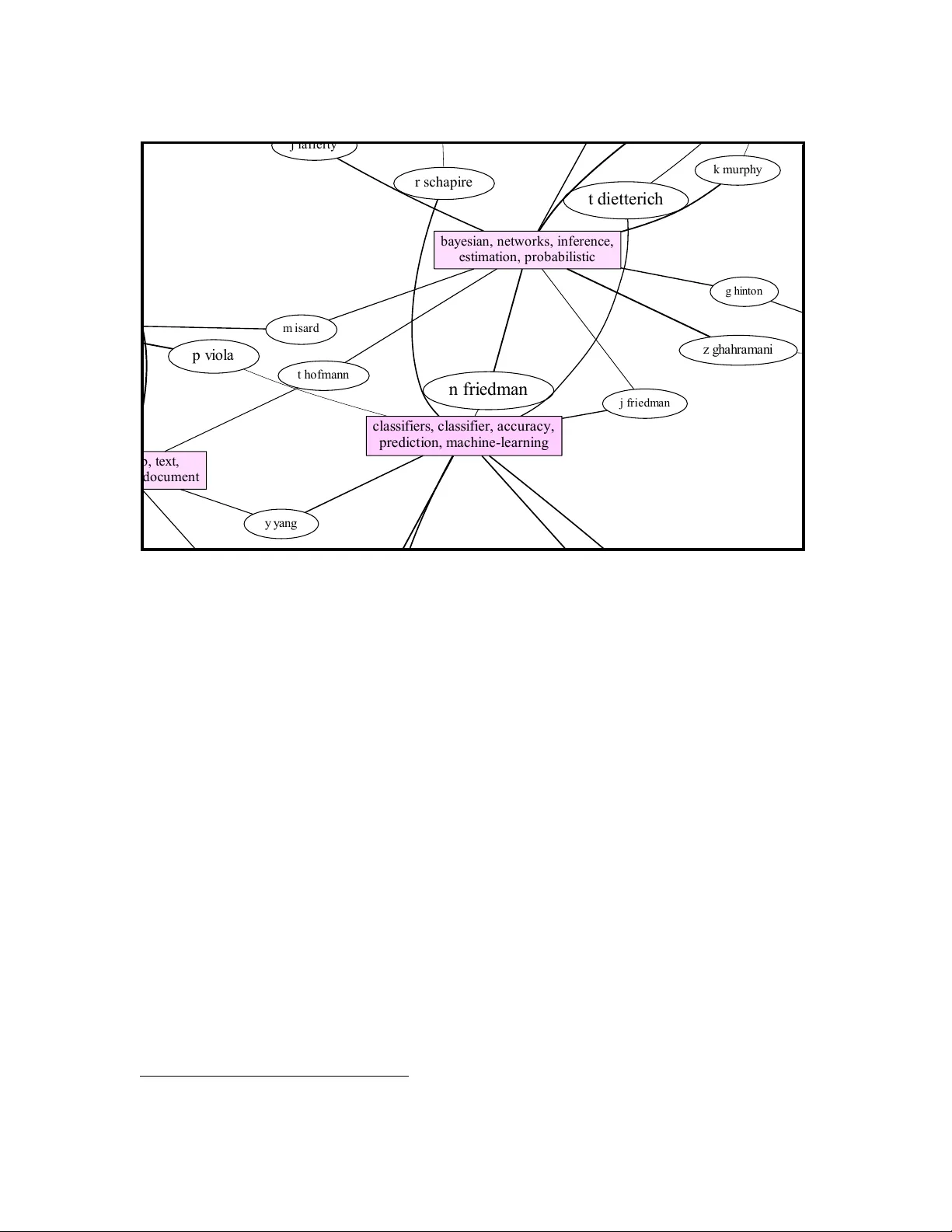
Preprint for article in Machine Learning 103 (2016) 185–213 Submitted 24 Mar 2015; Published 23 F eb 2016 Bibliographic Analysis on Researc h Publications using Authors, Categorical Lab els and the Citation Net work Kar W ai Lim kar w ai.lim@anu.edu.a u The A ustr alian National University and NICT A, Austr alia W ra y Bun tine wra y.buntine@monash.edu Monash University, A ustr alia Editor: Hang Li, Dinh Ph ung, T ru Cao, T u-Bao Ho, and Zhi-Hua Zhou Abstract Bibliographic analysis considers the author’s research areas, the citation net w ork and the pap er con ten t among other things. In this paper, w e com bine these three in a topic mo del that produces a bibliographic mo del of authors, topics and do cumen ts, using a nonparamet- ric extension of a combination of the Poisson mixed-topic link mo del and the author-topic mo del. This gives rise to the Citation Netw ork T opic Mo del (CNTM). W e prop ose a nov el and eﬃcient inference algorithm for the CNTM to explore subsets of research publications from CiteSeer X . The publication datasets are organised into three corp ora, totalling to ab out 168k publications with ab out 62k authors. The queried datasets are made av ailable online. In three publicly av ailable corp ora in addition to the queried datasets, our prop osed mo del demonstrates an improv ed p erformance in b oth mo del ﬁtting and do cumen t clus- tering, compared to several baselines. Moreo v er, our mo del allo ws extraction of additional useful knowledge from the corp ora, such as the visualisation of the author-topics net w ork. Additionally , we prop ose a simple metho d to incorp orate sup ervision into topic mo delling to ac hiev e further improv emen t on the clustering task. Keyw ords: Bibliographic analysis, T opic model, Bay esian nonparametric, Author-citation net w ork, Pitman-Y or pro cess 1. In troduction Mo dels of bibliographic data need to consider man y kinds of information. Articles are usually accompanied by metadata suc h as authors, publication data, categories and time. Cited pap ers can also b e av ailable. When authors’ topic preferences are mo delled, we need to asso ciate the do cumen t topic information someho w with the authors’. Join tly mo delling text data with citation net w ork information can b e challenging for topic mo dels, and the problem is confounded when also mo delling author-topic relationships. In this pap er, we prop ose a topic mo del to jointly mo del authors’ topic preferences, text con ten t 1 and the citation netw ork. The mo del is a nonparametric extension of previous mo dels discussed in Section 2 . Using simple assumptions and approximations, w e derive a no v el algorithm that allows the probabilit y vectors in the mo del to b e integrated out. This yields a Marko v c hain Monte Carlo (MCMC) inference via discrete sampling. 1. Abstract and publication title. c  2016 Lim and Buntine. DOI 10.1007/s10994-016-5554-z Lim and Buntine As an extension of our previous w ork ( Lim and Bun tine , 2014 ), w e prop ose a sup ervised approac h to improv e do cumen t clustering, by making use of categorical information that is av ailable. Our metho d allows the level of sup ervision to b e adjusted through a v ariable, giving us a mo del with no sup ervision, semi-sup ervised or fully sup ervised. Additionally , w e presen t a more extensive qualitativ e analysis of the learned topic mo dels, and displa y a visualisation snapshot of the learned author-topics netw ork. W e also p erform additional diagnostic tests to assess our prop osed topic mo del. F or example, we study the conv er- gence of the prop osed learning algorithm and rep ort on the computation complexity of the algorithm. In the next section, we discuss the related w ork. Section 3 , 4 and 5 detail our topic model and its inference algorithm. W e describ e the datasets in Section 6 and report on exp erimen ts in Section 7 . Applying our mo del on research publication data, w e demonstrate the mo del’s impro v ed p erformance, on b oth mo del ﬁtting and a clustering task, compared to several baselines. Additionally , in Section 8 , w e qualitatively analyse the inference results produced b y our model. W e ﬁnd that the learned topics ha v e high comprehensibilit y . Additionally , we presen t a visualisation snapshot of the learned topic mo dels. Finally , we p erform diagnostic assessmen t of the topic mo del in Section 9 and conclude the pap er in Section 10 . 2. Related W ork Laten t Dirichlet Allo cation (LDA) ( Blei et al. , 2003 ) is the simplest Bay esian topic mo del used in modelling text, whic h also allows easy learning of the mo del. T eh and Jordan ( 2010 ) prop osed the Hier ar chic al Dirichlet pr o c ess (HDP) LDA, which utilises the Diric hlet process (DP) as a nonparametric prior which allows a non-symmetric, arbitrary dimensional topic prior to b e used. F urthermore, one can replace the Dirichlet prior on the word vectors with the Pitman-Y or Pr o c ess (PYP , also kno wn as the tw o-parameter Poisson Dirichlet pro- cess) ( T eh , 2006b ), which mo dels the p o w er-la w of word frequency distributions in natural language ( Goldw ater et al. , 2011 ), yielding signiﬁcant improv emen t ( Sato and Nak agaw a , 2010 ). V ariants of LD A allow incorp orating more aspects of a particular task and here we consider authorship and citation information. The author-topic mo del (A TM) ( Rosen-Zvi et al. , 2004 ) uses the authorship information to restrict topic options based on author. Some recent w ork jointly mo dels the do cumen t citation netw ork and text conten t. This includes the r elational topic mo del ( Chang and Blei , 2010 ), the Poisson mixe d-topic link mo del (PMTLM) ( Zhu et al. , 2013 ) and Link-PLSA-LDA ( Nallapati et al. , 2008 ). An extensiv e review of these mo dels can b e found in Zhu et al. ( 2013 ). The Citation Author T opic (CA T) mo del ( T u et al. , 2010 ) mo dels the author-author netw ork on publications based on citations using an extension of the A TM. Note that our work is diﬀeren t to CA T in that we mo del the author-do cumen t-citation net w ork instead of author-author netw ork. The T opic-Link LDA ( Liu et al. , 2009 ) jointly mo dels author and text by using the distance b et w een the do cumen t and author topic vectors. Similarly the Twitter-Netw ork topic mo del ( Lim et al. , 2013 ) mo dels the author netw ork 2 based on author topic distribu- tions, but using a Gaussian pro cess to mo del the net w ork. Note that our work considers the author-do cument-citation of Liu et al. ( 2009 ). W e use the PMTLM of Zhu et al. ( 2013 ) 2. The author net w ork here corresponds to the Twitter follow er netw ork. 2 Bibliographic Anal ysis using Authors, Ca tegorical Labels and Cit a tion Network to mo del the net w ork, which lets one in tegrate PYP hierarchies with the PMTLM using eﬃcien t MCMC sampling. There is also existing w ork on analysing the degree of authors’ inﬂuence. On publication data, Kataria et al. ( 2011 ) and Mimno and McCallum ( 2007 ) analyse inﬂuential authors with topic mo dels, while W eng et al. ( 2010 ), T ang et al. ( 2009 ), and Liu et al. ( 2010 ) use topic mo dels to analyse users’ inﬂuence on so cial media. 3. Sup ervised Citation Netw ork T opic Mo del In our previous work ( Lim and Buntine , 2014 ), w e prop osed the Citation Netw ork T opic Mo del (CNTM) that jointly mo dels the text , authors , and the citation network of research publications (do cumen ts). The CNTM allows us to b oth mo del the authors and text b etter b y exploiting the correlation b etw een the authors and their researc h topics. How ever, the b eneﬁt of the abov e mo delling is not realised when the author information is simply missing from the data. This could b e due to error in data collection ( e.g. metadata not prop erly formatted), or even simply that the author information is lost during prepro cessing. In this section, we prop ose an extension of the CNTM that remedies the ab ov e issue, by making use of additional metadata that is a v ailable. F or example, the metadata could b e the researc h areas or keyw ords asso ciated with the publications, whic h are usually provided b y the authors during the publication submission. How ev er, this information might not alw a ys b e reliable as it is not standardised across diﬀeren t publishers or conferences. In this pap er, rather than using the mentioned metadata, we will instead incorp orate the categorical lab els that were previously used as ground truth for ev aluation. As such, our extension giv es rise to a sup ervised mo del, which we will call the Sup ervised Citation Netw ork T opic Mo del (SCNTM). W e ﬁrst describ e the topic mo del part of SCNTM for which the citations are not consid- ered, it will b e used for comparison later in Section 7 . W e then complete the SCNTM with the discussion on its netw ork comp onen t. The full graphical mo del for SCNTM is display ed in Figure 1 . T o clarify the notations used in this pap er, variables that ar e without subscript r epr esent a c ol le ction of variables of the same notation . F or instance, w d represen ts all the words in do cumen t d , that is, w d = { w d 1 , . . . , w dN d } where N d is the num b er of words in do cumen t d ; and w represen ts all words in a corpus, w = { w 1 , . . . , w D } , where D is the n um ber of do cumen ts. 3.1 Hierarc hical Pitman-Y or T opic Mo del The SCNTM uses b oth the Griﬃths-Engen-McCloskey (GEM) distribution ( Pitman , 1996 ) and the Pitman-Y or pr o c ess (PYP) ( T eh , 2006b ) to generate probability vectors. Both the GEM distribution and the PYP are parameterised by a disc ount parameter α and a c onc entr ation parameter β . The PYP is additionally parameterised b y a b ase distribution H , whic h is also the mean of the PYP when it can b e represented b y a probabilit y vector. Note that the base distribution can also b e a PYP . This giv es rise to the hierarc hical Pitman-Y or pro cess (HPYP). In mo delling authorship, the SCNTM mo diﬁes the approach of the author-topic mo del ( Rosen-Zvi et al. , 2004 ) which assumes that the words in a publication are equally attributed 3 Lim and Buntine Figure 1: Graphical mo del for SCNTM. The b o x on the top left with D 2 en tries is the citation net w ork on do cumen ts represented as a Bo olean matrix. The remainder is a nonparametric hierarc hical PYP topic mo del where the lab elled categories and authors are captured b y the topic v ectors ν . The topic v ectors ν inﬂuence the D do cumen ts’ topic v ectors θ 0 and θ based on the observ ed authors a or categories e . The latent topics and asso ciated words are represented by the v ariables z and w . The K topics, shown in the top righ t, ha ve bursty mo delling follo wing Bun tine and Mishra ( 2014 ). to the diﬀeren t authors. This is not reﬂected in practice since publications are often written more by the ﬁrst author, excepting when the order is alphab etical. Thus, we assume that the ﬁrst author is dominant and attribute all the w ords in a publication to the ﬁrst author. Although, w e could model the con tribution of eac h author on a publication by , sa y , using a Dirichlet distribution, w e found that considering only the ﬁrst author gives a simpler learning algorithm and cleaner results. The generative pro cess of the topic mo del comp onent of the SCNTM is as follows. W e ﬁrst sample a ro ot topic distribution µ with a GEM distribution to act as a base distribution for the author-topic distributions ν a for each author a , and also for the category-topic distributions ν e for each category e : µ ∼ GEM( α µ , β µ ) , (1) ν a | µ ∼ PYP( α ν a , β ν a , µ ) , a ∈ A . (2) ν e | µ ∼ PYP( α ν e , β ν e , µ ) , e ∈ E . (3) Here, A represents the set of all authors while E denotes the set of all categorical lab els in the text corpus. Note w e hav e used the same symbol ( ν ) for b oth the author-topic distributions and the category-topic distributions. W e in tro duce a parameter η called the author thr eshold whic h controls the level of sup ervision used by SCNTM. W e say an author a is signiﬁcant if the author has pro duced 4 Bibliographic Anal ysis using Authors, Ca tegorical Labels and Cit a tion Network more than or equal to η publications, i.e. signiﬁcance( a ) =  1 if P d I ( a d = a ) ≥ η 0 otherwise . (4) Here, a d represen ts the author for do cumen t d , and I ( 4 ) is the indicator function that ev aluates to 1 if 4 is true, else 0. Next, for eac h do cumen t d in a publication collection of size D , we sample the do cumen t- topic prior θ 0 d from ν a d or ν e d dep ending on whether the author a d for the do cumen t is signiﬁcan t: θ 0 d | a d , e d , ν ∼  PYP( α θ 0 d , β θ 0 d , ν a d ) if signiﬁcance( a d ) = 1 PYP( α θ 0 d , β θ 0 d , ν e d ) otherwise , d = 1 , . . . , D , (5) where e d is the categorical lab el asso ciated with do cumen t d . F or the sak e of notational simplicit y , we introduce a v ariable b to capture b oth the author and the category . W e let b tak es the v alue of 1 , . . . , A for each author in A , and let b takes the v alue of ( A + 1) , . . . , B for the categories in E . Note that B = |A| + |E | . Thus, w e can also write the distribution of θ 0 d as θ 0 d | ν b ∼ PYP( α θ 0 d , β θ 0 d , ν b ) d = 1 , . . . , D , (6) where b = a d if signiﬁcance( a d ) = 1, else b = e d . By modelling this wa y , we are able to handle missing authors and incorp orate sup ervision in to the SCNTM. F or example, choosing η = 1 allo ws us to make use of the categorical information for do cumen ts that hav e no v alid author. Alternativ ely , w e could select a higher η , this s mooths out the do cumen t-topic distributions for do cumen ts that are written b y authors who ha v e authored only a small n um ber of publications. This treatment leads to a b etter clustering result as these authors are usually not discriminativ e enough for prediction. On the extreme, we can set η = ∞ to ac hiev e full supervision. W e note that the SCNTM reverts to the CNTM when η = 0, in this case the mo del is not sup ervised. W e then sample the do cumen t-topic distribution θ d giv en θ 0 d : θ d | θ 0 d ∼ PYP( α θ d , β θ d , θ 0 d ) , d = 1 , . . . , D . (7) Note that instead of mo delling a single do cumen t-topic distribution, we mo del a do cumen t- topic hierarc h y with θ 0 and θ . The primed θ 0 represen ts the topics of the do cument in the con text of the citation netw ork. The unprimed θ represen ts the topics of the text, naturally related to θ 0 but not the same. Suc h modelling gives citation information a higher impact to tak e in to account the relativ ely low amount of citations compared to the text. The tec hnical details on the eﬀect of such mo delling is presented in Section 9.2 . F or the vocabulary side, w e generate a background word distribution γ given H γ , a discrete uniform vector of length |V | , i.e. H γ = ( · · · , 1 |V | , · · · ). V is the set of distinct word tok ens observed in a corpus. Then, w e sample a topic-w ord distribution φ k for each topic k , with γ as the base distribution: γ ∼ PYP( α γ , β γ , H γ ) , (8) φ k | γ ∼ PYP( α φ k , β φ k , γ ) , k = 1 , . . . , K . (9) 5 Lim and Buntine Mo delling word burstiness ( Buntine and Mishra , 2014 ) is imp ortan t since w ords in a doc- umen t are likely to rep eat in the do cumen t. The same applies to publication abstract, as shown in Section 6 . T o address this prop ert y , w e mak e the topics bursty so eac h do c- umen t only fo cuses on a subset of w ords in the topic. This is achiev ed by deﬁning the do cumen t-sp eciﬁc topic-word distribution φ 0 dk for each topic k in do cumen t d as: φ 0 dk | φ k ∼ PYP( α φ 0 dk , β φ 0 dk , φ k ) , d = 1 , . . . , D , k = 1 , . . . , K . (10) Finally , for each w ord w dn in do cumen t d , w e sample the corresp onding topic assignment z dn from the do cumen t-topic distribution θ d ; while the w ord w dn is sampled from the topic-w ord distribution φ 0 d giv en z dn : z dn | θ d ∼ Discrete( θ d ) , (11) w dn | z dn , φ 0 d ∼ Discrete( φ 0 dz dn ) , d = 1 , . . . , D , n = 1 , . . . , N d . (12) Note that w includes w ords from the publications’ title and abstract, but not the full article. This is b ecause title and abstract provide a go o d summary of a publication’s topics and th us more suited for topic mo delling, while the full article con tains to o m uc h technical detail that might not b e to o relev ant. In the next section, w e describ e the mo delling of the citation netw ork accompanying a publication collections. This completes the SCNTM. 3.2 Citation Net w or k Poisson Mo del T o mo del the citation netw ork b etw een publications, we assume that the citations are generated conditioned on the topic distributions θ 0 of the publications. Our approach is motiv ated by the degree-corrected v ariant of PMTLM ( Zh u et al. , 2013 ). Denoting x ij as the num ber of times document i citing document j , we model x ij with a P oisson distribution with mean parameter λ ij : x ij | λ ij ∼ P oisson( λ ij ) , λ ij = λ + i λ − j P k λ T k θ 0 ik θ 0 j k , i = 1 , . . . , D , j = 1 , . . . , D . (13) Here, λ + i is the prop ensity of do cumen t i to cite and λ − j represen ts the p opularit y of cited do cumen t j , while λ T k scales the k -th topic, eﬀectively p enalising common topics and strengthen rare topics. Hence, a citation from do cument i to do cumen t j is more likely when these do cumen ts are having relev ant topics. Due to the limitation of the data, the x ij can only b e 0 or 1, i.e. it is a Bo olean v ariable. Nevertheless, the Poisson distribution is used instead of a Bernoulli distribution b ecause it leads to dramatically reduced complexity in analysis ( Zhu et al. , 2013 ). Note that the Poisson distribution is similar to the Bernoulli distribution when the mean parameter is small. W e present a list of v ariables asso ciated with the SCNTM in T able 1 . 4. Mo del Representation and Posterior Lik eliho o d Before presen ting the p osterior used to dev elop the MCMC sampler, w e brieﬂy review handling of the hierarchical PYP mo dels in Section 4.1 . W e cannot pro vide an adequately detailed review in this pap er, thus we presen t the main ideas. 6 Bibliographic Anal ysis using Authors, Ca tegorical Labels and Cit a tion Network T able 1: List of V ariables for the Sup ervised Citation Netw ork T opic Mo del (SCNTM). V ariable Name Description z dn T opic T opical lab el for word w dn . w dn W ord Observed word or phrase at p osition n in do cumen t d . x ij Citations Num b er of times do cumen t i cites do cumen t j . a d Author Author for do cumen t d . e d Category Category lab el for do cument d . φ 0 dk Do cumen t-topic- w ord distribution Probabilit y distribution in generating words given do cumen t d and topic k . φ k T opic-word distribution W ord prior for φ 0 dk . θ d Do cumen t-topic distribution Probabilit y distribution in generating topics for do cumen t d . θ 0 d Do cumen t-topic prior T opic prior for θ d . ν b Author/category- topic distribution Probabilit y distribution in generating topics for author or category b . γ Global word distribution W ord prior for φ k . µ Global topic distribution T opic prior for ν b . α N Discoun t Discoun t parameter of the PYP N . β N Concen tration Concen tration parameter of the PYP N . H N Base distribution Base distribution of the PYP N . λ ij Rate Rate parameter or the mean for x ij . λ + i Cite prop ensit y Prop ensit y to cite for do cumen t i . λ − i Cited prop ensit y Prop ensit y to b e cited for do cument j . λ T k Scaling factor Citation scaling factor for topic k . 4.1 Mo delling with Hierarc hical PYPs The key to eﬃcient sampling with PYPs is to marginalise out the probabilit y v ectors ( e.g. topic distributions) in the model and record v arious asso ciated counts instead, th us yielding a collapsed sampler. While a common approac h here is to use the hierarc hical Chinese Restauran t Pro cess (CRP) of T eh and Jordan ( 2010 ), w e use another representation that requires no dynamic memory and has b etter inference eﬃciency ( Chen et al. , 2011 ). 7 Lim and Buntine W e denote f ∗ ( N ) as the marginalised likelihoo d asso ciated with the probability vector N . Since the v ector is marginalised out, the marginalised likelihoo d is in terms of — using the CRP terminology — the customer c ounts c N = ( · · · , c N k , · · · ) and the table c ounts t N = ( · · · , t N k , · · · ). The customer coun t c N k corresp onds to the num ber of data p oin ts ( e.g. w ords) assigned to group k ( e.g. topic) for v ariable N . Here, the table c ounts t N represen t the subset of c N that gets passed up the hierarch y (as customers for the parent probabilit y v ector of N ). Thus t N k ≤ c N k , and t N k = 0 if and only if c N k = 0 since the coun ts are non-negativ e. W e also denote C N = P k c N k as the total customer counts for no de N , and similarly , T N = P k t N k is the total table counts. The marginalised lik eliho od f ∗ ( N ), in terms of c N and t N , is given as f ∗ ( N ) = ( β N | α N ) T N ( β N ) C N Y k S c N k t N k ,α N , for N ∼ PYP( α N , β N , P ) . (14) S x y ,α is the generalised Stirling n um b er that is easily tabulated; b oth ( x ) C and ( x | y ) C denote the Pochhammer symbol (rising factorial), see Buntine and Hutter ( 2012 ) for details. Note the GEM distribution behav es lik e a PYP in whic h the table count t N k is alwa ys 1 for non-zero c N k . The innov ation of Chen et al. ( 2011 ) w as to notice that sampling with Equation ( 14 ) directly led to p oor p erformance. The problem was that sampling an assignmen t to a latent v ariable, sa y moving a customer from group k to k 0 (so c N k decreases by 1 and c N k 0 increases b y 1), the p oten tial eﬀect on t N k and t N k 0 could not immediately b e measured. Whereas, the hierarchical CRP automatically included table conﬁgurations in its sampling pro cess and th us included the inﬂuence of the hierarc h y in the sampling. Thus sampling directly with Equation ( 14 ) lead to comparatively p o or mixing. As a solution, Chen et al. ( 2011 ) dev elop a collapsed version of the hierarchical CRP follo wing the well known practice of Rao-Blac kw ellisation of sampling schemes ( Casella and Rob ert , 1996 ), which, while not b eing as fast p er step, it has tw o distinct adv an tages, (1) it requires no dynamic memory and (2) the sampling has signiﬁcantly low er v ariance so conv erges muc h faster. This has empirically b een shown to lead to b etter mixing of the samplers ( Chen et al. , 2011 ) and has b een conﬁrmed on diﬀerent complex topic mo dels ( Buntine and Mishra , 2014 ). The technique for collapsing the hierarc hical CRP uses Equation ( 14 ) but the coun ts ( c N , t N ) are no w deriv ed v ariables. They are deriv ed from Boolean v ariables asso ciated with eac h data p oin t. The technique comprises the following conceptual steps: (1) add Bo olean indicators u dn to the data ( z dn , w dn ) from which the counts c N and t N can b e deriv ed, (2) mo dify the marginalised p osterior accordingly , and (3) derive a sampler for the mo del. 4.1.1 Adding Boolean indica tors W e ﬁrst consider c θ d k , which has a “+1” contributed to for every z dn = k in do cumen t d , hence c θ d k = P n I ( z dn = k ). W e now introduce a new Bernoulli indic ator variable u θ d dn asso ciated with z dn , which is “on” (or 1) when the data z dn also contributed a “+1” to t θ d k . Note that t θ d k ≤ c θ d k , so every data contributing a “+1” to c θ d k ma y or ma y not con tribute a “+1” to t θ d k . The result is that one derives t θ d k = P n I ( z dn = k ) I ( u θ d dn = 1). No w consider the paren t of θ d , which is θ 0 d . Its customer count is deriv ed as c θ 0 d k = t θ d k . Its table count t θ 0 d k can now b e treated similarly . Those data z dn that contribute a “+1” 8 Bibliographic Anal ysis using Authors, Ca tegorical Labels and Cit a tion Network to t θ d k (and th us c θ 0 d k ) ha v e a new Bernoulli indicator v ariable u θ 0 d dn , which is used to derive t θ 0 d k = P n I ( z dn = k ) I ( u θ 0 d dn = 1), similar as b efore. Note that if u θ 0 d dn = 1 then necessarily u θ d dn = 1. Similarly , one can deﬁne Bo olean indicators for µ , ν b , φ 0 , φ , and γ to ha v e a full suite from whic h all the counts c N and t N are now derived. W e denote u dn = { u θ d dn , u θ 0 d dn , u ν b dn , u µ dn , u φ 0 d dn , u φ d dn , u γ dn } as the collection of the Bo olean indicators for data ( z dn , w dn ). 4.1.2 Probability of Boolean indica tors By symmetry , if there are t N k Bo olean indicators “on” (out of c N k ), we are indiﬀerent as to whic h is on. Thus the indicator v ariable u N dn is not stored, that is, we simply “forget” who con tributed a table count and re-sample u N dn as needed: p ( u N dn = 1) = t N k /c N k , p ( u N dn = 0) = 1 − t N k /c N k . (15) Moreo v er, this means that the marginalised likelihoo d f ∗ ( N ) of Equation ( 14 ) is extended to include the probability of u N , which is written in terms of c N , t N and u N as: f ( N ) = f ∗ ( N ) p  u N   c N , t N  = f ∗ ( N ) Y k  c N k t N k  − 1 . (16) 4.2 Lik eliho od for the Hierarchical PYP T opic Mo del W e use b old face capital letters to denote the set of all relev ant low er case v ariables. F or example, Z = { z 11 , · · · , z DN D } denotes the set of all topic assignments. V ariables W , T , C and U are similarly deﬁned, that is, they denote the set of all w ords, table counts, customer coun ts, and Bo olean indicators resp ectiv ely . Additionally , we denote ζ as the set of all h yp erparameters (suc h as the α ’s). With the probabilit y vectors replaced b y the coun ts, the lik elihoo d of the topic model can be written — in terms of f ( · ) as given in Equation ( 16 ) — as p ( Z , W , T , C , U | ζ ) ∝ f ( µ ) B Y b =1 f ( ν b ) ! D Y d =1 f ( θ 0 d ) f ( θ d ) K Y k =1 f ( φ 0 dk ) ! K Y k =1 f ( φ k ) ! f ( γ ) Y v  1 |V |  t γ v ! . (17) Note that the last term in Equation ( 17 ) corresp onds to the parent probability vector of γ (see Section 3.1 ), and v indexes the unique w ord tokens in vocabulary set V . Note that the extra terms for U are simply derived using Equation ( 16 ) and not stored in the mo del. So in the discussions b elo w we will usually represent U implicitly b y T and C , and introduce the U when explicitly needed. Note that ev en though the probability vectors are integrated out and not explicitly stored, they can easily b e estimated from the asso ciated coun ts. The probabilit y vector N can b e estimated from its p osterior mean given the counts and parent probabilit y vector P : ˆ N =  · · · , ( α N T N + β N ) P k + c N k − α N T N k β N + C N , · · ·  . (18) 9 Lim and Buntine 4.3 Lik eliho od for the Citation Netw ork Poisson Mo del F or the citation netw ork, the Poisson likelihoo d for each x ij is given as p ( x ij | λ, θ ) = λ x ij ij x ij ! e λ ij ≈ λ + i λ − j X k λ T k θ 0 ik θ 0 j k ! x ij exp − λ + i λ − j X k λ T k θ 0 ik θ 0 j k ! . (19) Note that the term x ij ! is dropp ed in Equation ( 19 ) due to the limitation of the data that x ij ∈ { 0 , 1 } , thus x ij ! is ev aluated to 1. With conditional indep endence of x ij , the join t lik elihoo d for the whole citation netw ork X = { x 11 , · · · , x DD } can b e written as p ( X | λ, θ 0 ) = Y i ( λ + i ) g + i ( λ − i ) g − i ! Y ij X k λ T k θ 0 ik θ 0 j k ! x ij exp − X ij k λ + i λ − j λ T k θ 0 ik θ 0 j k ! , (20) where g + i is the num ber of citations for publication i , g + i = P j x ij , and g − i is the num ber of times publication i b eing cited, g − i = P j x j i . W e also make a simplifying assumption that x ii = 1 for all do cumen ts i , that is, all publications are treated as self-cited. This assumption is imp ortan t since deﬁning x ii allo ws us to rewrite the joint likelihoo d into Equation ( 20 ), whic h leads to a cleaner learning algorithm that utilises an eﬃcient cac hing. Note that if we do not deﬁne x ii , we hav e to explicitly consider the case when i = j in Equation ( 20 ) which results in messier summation and pro ducts. Note the likelihoo d in Equation ( 20 ) contains the do cumen t-topic distribution θ 0 in v ector form. This is problematic as p erforming inference with the likelihoo d requires the probabilit y vectors θ 0 , ν and µ to b e stored explicitly (instead of coun ts as discussed in Section 4.1 ). T o ov ercome this issue, w e prop ose a nov el representation that allows the probabilit y vectors to remain integrated out. Suc h representation also leads to an eﬃcient sampling algorithm for the citation netw ork, as we will see in Section 5 . W e in tro duce an auxiliary variable y ij , named the citing topic , to denote the topic that prompts publication i to cite publication j . T o illustrate, for a biolo gy publication that cites a machine le arning publication for the learning tec hnique, the citing topic w ould b e ‘mac hine learning’ instead of ‘biology’. F rom Equation ( 13 ), w e mo del the citing topic y ij as jointly Poisson with x ij : x ij , y ij = k | λ, θ 0 ∼ P oisson  λ + i λ − j λ T k θ 0 ik θ 0 j k  . (21) Incorp orating Y , the set of all y ij , we rewrite the citation net w ork lik eliho od as p ( X , Y | λ, θ 0 ) ∝ Y i ( λ + i ) g + i ( λ − i ) g − i Y k  λ T k  1 2 P i h ik Y ik θ 0 ik h ik exp − X ij λ + i λ − j λ T y ij θ 0 iy ij θ 0 j y ij ! , (22) where h ik = P j x ij I ( y ij = k ) + P j x j i I ( y j i = k ) is the num ber of connections publication i made due to topic k . T o integrate out θ 0 , we note the term θ 0 ik h ik app ears like a multinomial likelihoo d, so we absorb them in to the lik eliho od for p ( Z , W , T , C , U | ζ ) where they correspond to additional 10 Bibliographic Anal ysis using Authors, Ca tegorical Labels and Cit a tion Network coun ts for c θ 0 i , with h ik added to c θ 0 i k . T o disambiguate the source of the counts, w e will refer to these customer counts contributed by x ij as network c ounts , and denote the augmented coun ts ( C plus netw ork counts) as C + . F or the exp onential term, we use the delta metho d ( Oehlert , 1992 ) to approximate R q ( θ ) exp( − g ( θ )) d θ ≈ exp( − g ( ˆ θ )) R q ( θ ) d θ , where ˆ θ is the exp ected v alue according to a distribution prop ortional to q ( θ ). This approximation is rea- sonable as long as the terms in the exp onen tial are small (see App endix A ). The approximate full p osterior of SCNTM can then b e written as p ( Z , W , T , C + , U , X , Y | λ, ζ ) ≈ p ( Z , W , T , C + , U | ζ ) Y i ( λ + i ) g + i ( λ − i ) g − i Y k ( λ T k ) g T k exp − X ij λ + i λ − j λ T y ij ˆ θ 0 iy ij ˆ θ 0 j y ij ! , (23) where g T k = 1 2 P i h ik . W e note that p ( Z , W , T , C + , U | ζ ) is the same as Equation ( 17 ) but no w with C + instead of C . In the next section, w e demonstrate that our mo del represen tation gives rise to an in tuitiv e sampling algorithm for learning the mo del. W e also show how the Poisson mo del in tegrates in to the topic mo delling framework. 5. Inference T ec hniques Here, we derive the Marko v chain Mon te Carlo (MCMC) algorithms for learning the SC- NTM. W e ﬁrst describ e the sampler for the topic mo del and then for the citation netw ork. The full inference pro cedure is p erformed b y alternating b et ween the t w o samplers. Finally , w e outline the h yp erparameter samplers that are used to estimate the h yp erparameters automatically . 5.1 Sampling for the Hierarc hical PYP T opic Mo del T o sample the words’ topic Z and the asso ciated coun ts T and C in the SCNTM, we design a Metrop olis-Hastings (MH) algorithm based on the collapsed Gibbs sampler designed for the PYP ( Chen et al. , 2011 ). The concept of the MH sampler is analogous to LDA, which consists of (1) decrementing the counts asso ciated with a word, (2) sampling the resp ectiv e new topic assignment for the word, and (3) incremen ting the asso ciated counts. How ever, our sampler is more complicated than LD A. In particular, we ha v e to consider the indicators u N dn describ ed in Section 4.1 op erating on the hierarch y of PYPs. Our MH sampler consists of t w o steps. First w e sample the latent topic z dn asso ciated with the word w dn . W e then sample the customer counts C and table counts T . The sampler pro ceeds by considering the laten t v ariables asso ciated with a given word w dn . First, w e decrement the coun ts asso ciated with the word w dn and the latent topic z dn . This is achiev ed b y sampling the suite of indicators u dn according to Equation ( 15 ) and decremen ting the relev an t customer counts and table coun ts. F or example, w e decrement c θ d z dn b y 1 if u θ d dn = 1. After decrementing, w e apply a Gibbs sampler to sample a new topic z dn from its conditional p osterior distribution, given as p ( z new dn | Z − dn , W , T − dn , C + − dn , U − dn , ζ ) = X u dn p  z new dn , u dn   Z − dn , W , T − dn , C + − dn , U − dn , ζ  . (24) 11 Lim and Buntine Note that the join t distribution in Equation ( 24 ) can b e written as the ratio of the lik eliho o d for the topic mo del (Equation ( 17 )): p ( Z , W , T , C + , U | ζ ) p ( Z − dn , W , T − dn , C + − dn , U − dn | ζ ) . (25) Here, the sup erscript  − dn indicates that the topic z dn , indicators and the asso ciated coun ts for w ord w dn are not observed in the resp ective sets, i.e. the state after decremen t. Addi- tionally , we use the sup erscripts  new and  old to denote the prop osed sample and the old v alue resp ectiv ely . The mo dularised likelihoo d of Equation ( 17 ) allo ws the conditional p os- terior (Equation ( 24 )) to b e computed easily , since it simpliﬁes to ratios of likelihoo d f ( · ), whic h simpliﬁes further since the coun ts diﬀer by at most 1 during sampling. F or instance, the ratio of the P ochhammer sym b ols, ( x | y ) C +1 / ( x | y ) C , simpliﬁes to x + C y , while the ratio of Stirling num b ers, such as S y +1 x +1 ,α /S y x,α , can be computed quic kly via cac hing ( Buntine and Hutter , 2012 ). Next, w e pro ceed to sample the relev ant customer coun ts and table counts given the new z dn = k . W e prop ose an MH algorithm for this. W e deﬁne the prop osal distribution for the new customer coun ts and table counts as q  T new , C + new    Z , W , T − dn , C + − dn , ζ  ∝ p  Z , W , T new , C + new , U new   ζ  p  Z , W , T − dn , C + − dn , U − dn   ζ  (26) where p ( Z , W , T , C + , U | ζ ) ∝ f ( µ ) B Y b =1 f ( ν b ) ! D Y d =1 f ( θ 0 d ) f ( θ d ) K Y k =1 f ( φ 0 dk ) ! K Y k =1 f ( φ k ) ! f ( γ ) Y v  1 |V |  t γ v ! . (27) Here, the p oten tial sample space for T new and C new are restricted to just t k + i and c k + i where i is either 0 or 1. Doing so allows us to av oid considering the exp onen tially many p ossibilities of T and C . The acceptance probabilit y asso ciated with the newly sampled T new and C new is A = p  Z , W , T new , C + new , U new   ζ  p  Z , W , T old , C + old , U old   ζ  · q  T old , C + old   Z , W , T − dn , C + − dn ζ  q  T new , C + new   Z , W , T − dn , C + − dn ζ  = 1 . (28) Th us w e alw a ys accept the prop osed sample. 3 Note that since µ is GEM distributed, incremen ting t µ k is equiv alen t to sampling a new topic, i.e. the num ber of topics increases b y 1. 3. The algorithm is named MH algorithm instead of Gibbs sampling due to the fact that the sample space for the counts is restricted and th us w e are not sampling from the posterior directly . 12 Bibliographic Anal ysis using Authors, Ca tegorical Labels and Cit a tion Network 5.2 Sampling for the Citation Net w ork F or the citation netw ork, w e prop ose another MH algorithm. The MH algorithm can b e summarised in three steps: (1) estimate the do cumen t topic prior θ 0 , (2) prop ose a new citing topic y ij , and (3) accept or reject the prop osed y ij follo wing an MH scheme. Note that the MH algorithm is similar to the sampler for the topic model, where w e decrement the counts, sample a new state and up date the counts. Since all probabilit y v ectors are represen ted as counts, we do not need to deal with their vector form. Additionally , our MH algorithm is in tuitiv e and simple to implement. Lik e the w ords in a do cumen t, each citation is assigned a topic, hence the w ords and citations can b e thought as voting to determine a do cumen ts’ topic. W e describ e our MH algorithm for the citation netw ork as follo ws. First, for each do cumen t d , w e estimate the exp ected do cumen t-topic prior ˆ θ 0 d from Equation ( 18 ). Then, for eac h do cumen t pair ( i, j ) where x ij = 1, we decrement the net w ork coun ts associated with x ij , and re-sample y ij with a prop osal distribution derived from Equation ( 21 ): p ( y new ij = k | ˆ θ 0 i , ˆ θ 0 j ) ∝ λ T k ˆ θ 0 ik ˆ θ 0 j k exp  − λ + i λ − j λ T k ˆ θ 0 ik ˆ θ 0 j k  , (29) whic h can b e further simpliﬁed since the terms inside the exp onen tial are very small, hence the exp term appro ximates to 1. W e empirically insp ected the exp onential term and we found that almost all of them are b et w een 0 . 99 and 1. This means the ratio of the exp o- nen tials is not signiﬁcant for sampling new citing topic y new ij . So we ignore the exp onen tial term and let p ( y new ij = k | ˆ θ 0 i , ˆ θ 0 j ) ∝ λ T k ˆ θ 0 ik ˆ θ 0 j k . (30) W e compute the acceptance probability A for the newly sampled y new ij = y 0 , changed from y old ij = y ∗ , and the successive change to the do cumen t-topic priors (from ˆ θ 0 old to ˆ θ 0 new ): A = exp  − P ij k λ + i λ − j λ T k ˆ θ 0 ik new ˆ θ 0 j k new  exp  − P ij k λ + i λ − j λ T k ˆ θ 0 ik old ˆ θ 0 j k old  p ( Z , W , T , C + new , U | ζ ) p ( Z , W , T , C + old , U | ζ ) × λ T y ∗ ˆ θ 0 iy ∗ new ˆ θ 0 j y ∗ new λ T y 0 θ 0 iy 0 old θ 0 j y 0 old P k λ T k ˆ θ 0 ik old ˆ θ 0 j k old P k λ T k ˆ θ 0 ik new ˆ θ 0 j k new . (31) Note that we hav e abused the notations i and j in the ab o v e equation, where the i and j in the summation indexes all do cumen ts instead of p oin ting to particular do cumen t i and do cument j . W e decided against in troducing additional v ariables to make things less confusing. Finally , if the sample is accepted, we up date y ij and the asso ciated custome r coun ts. Otherwise, we discard the sample and revert the changes. 5.3 Hyp erparameter Sampling Hyp erparameter sampling for the priors are imp ortan t ( W allac h et al. , 2009 ). In our infer- ence algorithm, w e sample the concentration parameters β of all PYPs with an auxiliary 13 Lim and Buntine Algorithm 1 Inference Algorithm for the Citation Netw ork T opic Mo del 1. Initialise the mo del b y assigning a random topic assignmen t z dn to eac h w ord w dn and constructing the relev ant customer counts c N k and table counts t N k for all v ariables N . 2. F or eac h w ord w dn in each do cumen t d : i. Decrement the counts asso ciated with z dn and w dn . ii. Sample a new topic z dn with its conditional p osterior in Equation ( 24 ). iii. Sample the counts T and C with the prop osal distribution in Equation ( 26 ). 3. F or eac h citation x ij = 1: i. Decrement the netw ork counts asso ciated with x ij and y ij . ii. Sample a new citing topic y ij with the prop osal distribution in Equation ( 30 ). iii. Accept or reject the sampled y ij with the acceptance probability in Equation ( 31 ). 4. Up date the hyperparameters β , λ + , λ − and λ T . 5. Rep eat steps 2-4 until the mo del conv erges or a ﬁx num b er of iterations reac hed. v ariable sampler ( T eh , 2006a ), but leav e the discoun t parameters α ﬁxed. W e do not sample the α due to the coupling of the parameter with the Stirling num b ers cache. Here we outline the pro cedure to sample the concen tration parameter β N of a PYP distributed v ariable N , using an auxiliary v ariable sampler. Assuming eac h β N has a Gamma distributed hyperprior with shap e τ 0 and rate τ 1 , we ﬁrst sample the auxiliary v ariables ξ and ψ j for j ∈ { 0 , T N − 1 } : ξ | β N ∼ Beta( C N , β N ) , ψ j | α N , β N ∼ Bernoulli  β N β N + j α N  . (32) W e then sample a new β 0 N from the following conditional p osterior given the auxiliary v ariables: β 0 N | ξ , ψ ∼ Gamma  τ 0 + P j ψ j , τ 1 − log (1 − ξ )  . (33) In addition to the PYP hyperparameters, we also sample λ + , λ − and λ T with a Gibbs sampler. W e let the hyperpriors for λ + , λ − and λ T to b e Gamma distributed with shap e  0 and rate  1 . With the conjugate Gamma prior, the p osteriors for λ + i , λ − i and λ T k are also Gamma distributed, so they can b e sampled directly . ( λ + i | X , λ − , λ T θ 0 ) ∼ Gamma   0 + g + i ,  1 + P k λ T k θ 0 ik P j λ − j θ 0 j k  , (34) ( λ − i | X , λ + , λ T θ 0 ) ∼ Gamma   0 + g − i ,  1 + P k λ T k θ 0 ik P j λ + j θ 0 j k  , (35) ( λ T k | X , Y , λ + , λ − , θ 0 ) ∼ Gamma   0 + 1 2 P i h ik ,  1 + λ T k ( P j λ + j θ 0 j k )( P j λ − j θ 0 j k )  . (36) W e apply v ague priors to the hyperpriors by setting τ 0 = τ 1 =  0 =  1 = 1. Before we pro ceed with the next section on the datasets used in the paper, w e summarise the full inference algorithm for the SCNTM in Algorithm 1 . 14 Bibliographic Anal ysis using Authors, Ca tegorical Labels and Cit a tion Network T able 2: Summary of the datasets used in the pap er, showing the num b er of publications, citations, authors, unique word tok ens, the a v erage n um ber of w ords in each docu- men t, and the av erage p ercen tage of unique words rep eated in a do cument. Note: author information is not a v ailable in the last three datasets. Datasets Publications Citations Authors V o cabulary W ords/Do c %Rep eat ML 139 227 1 105 462 43 643 8 322 59 . 4 23 . 3 M10 10 310 77 222 6 423 2 956 57 . 8 24 . 3 AvS 18 720 54 601 11 898 4 770 58 . 9 17 . 0 CS 3 312 4 608 − 3 703 31 . 8 − Cora 2 708 5 429 − 1 433 18 . 2 − PubMed 19 717 44 335 − 4 209 67 . 6 40 . 1 6. Data W e p erform our exp erimen ts on subsets of CiteSeer X data 4 whic h consists of scien tiﬁc pub- lications. Each publication from CiteSeer X is accompanied by title , abstr act , keywor ds , au- thors , citations and other metadata. W e prepare three publication datasets from CiteSeer X for ev aluations. The ﬁrst dataset corresp onds to Mac hine Learning (ML) publications, whic h are queried from CiteSeer X using the keyw ords from Microsoft Academic Search. 5 The ML dataset contains 139,227 publications. Our second dataset corresp onds to pub- lications from ten distinct research areas. The query w ords for these ten disciplines are c hosen such that the publications form distinct clusters. W e name this dataset M10 (Mul- tidisciplinary 10 classes), which is made of 10,310 publications. F or the third dataset, we query publications from b oth arts and science disciplines. Arts publications are made of history and r eligion publications, while the science publications contain physics , chemistry and biolo gy research. This dataset consis ts of 18,720 publications and is named AvS (Arts v ersus Science) in this pap er. These queried datasets are made a v ailable online. 6 The k eyw ords used to create the datasets are obtained from Microsoft Academic Searc h, and are listed in Appendix B . F or the clustering ev aluation in Section 7.4 , we treat the query categories as the ground truth. How ev er, publications that span multiple disciplines can b e problematic for clustering ev aluation, hence w e simply remov e the publications that satisfy the queries from more than one discipline. Nonetheless, the lab els are inherently noisy . The metadata for the publications can also b e noisy , for instance, the authors ﬁeld may some- times displa y publication’s keyw ords instead of the authors, publication title is sometimes an URL, and table of conten ts can b e mistak enly parsed as the abstract. W e discuss our treatmen ts to these issues in Section 6.1 . W e also note that non-English publications are discarded using langid.py ( Lui and Baldwin , 2012 ). In addition to the manually queried datasets, we also mak e use of existing datasets from LINQS ( Sen et al. , 2008 ) 7 to facilitate comparison with existing work. In particular, we 4. http://citeseerx.ist.psu.edu/ 5. http://academic.research.microsoft.com/ 6. http://karwai.weebly.com/publications.html 7. http://linqs.cs.umd.edu/projects/projects/lbc/ 15 Lim and Buntine T able 3: Categories of the datasets. Datasets Classes Categorical Lab els ML 1 Mac hine Learning M10 10 Agriculture, Archaeology , Biology , Computer Science, Physics, Financial Economics, Industrial Engineering, Material Science, P etroleum Chemistry , So cial Science AvS 5 History , Religion, Physics, Chemistry , Biology CS 6 Agen ts, AI, DB, IR, ML, HCI Cora 7 Case Based, Genetic Algorithms, Neural Netw orks, Theory , Probabilistic Metho ds, Reinforcemen t Learning, Rule Learning PubMed 3 “Diab etes Mellitus, Exp erimen tal”, Diab etes Mellitus T yp e 1, Diab etes Mellitus Type 2 use their CiteSeer, Cora and PubMed datasets. Their CiteSeer data consists of Computer Science publications and hence w e name the dataset CS to remov e ambiguit y . Although these datasets are small, they are fully lab elled and thus useful for clustering ev aluation. Ho w ev er, these three datasets do not come with additional metadata suc h as the authorship information. Note that the CS and Cora datasets are presen ted as Boolean matrices, i.e. the word counts information is lost and we assume that all words in a do cument o ccur only once. Additionally , the w ords ha v e b een conv erted to in teger so they do not conv ey an y semantics. Although this representation is less useful for topic mo delling, w e still use them for the sake of comparison. F or the PubMed dataset, w e recov er the w ord counts from TF-IDF using a simple assumption (see App endix C ). W e present a summary of the datasets in T able 2 and their resp ective categorical lab els in T able 3 . 6.1 Data Noise Remo v al Here, we brieﬂy discuss the steps taken to reduce the corrupted en tries in the CiteSeer X datasets (ML, M10 and AvS). Note that the keywor ds ﬁeld in the publications are often empt y and are sometimes noisy , that is, they contain irrelev ant information such as section heading and title, which makes the keyw ords unreliable source of information as categories. Instead, w e simply treat the k eyw ords as part of the abstracts. W e also remo v e the URLs from the data since they do not provide an y additional useful information. Moreo v er, the author information is not consistently presen ted in CiteSeer X . Some of the authors are shown with full name, some with ﬁrst name initialised, while some others are preﬁxed with title (Prof, Dr. etc. ). W e thus standardise the author information by remo ving all title from the authors, initialising all ﬁrst names and discarding the middle names. Although standardisation allows us to match up the authors, it do es not s olv e the problem that diﬀerent authors who hav e the same initial and last name are treated as a single author. F or example, b oth Bruce Lee and Brett Lee are standardised to B Lee. Note this corresp onds to a whole researc h problem ( Han et al. , 2004 , 2005 ) and hence not addressed in this pap er. Occas ionally , institutions are mistak enly treated as authors in CiteSeer X data, 16 Bibliographic Anal ysis using Authors, Ca tegorical Labels and Cit a tion Network example includes Americ an Mathematic al So ciety and T e chnische Universit¨ at M¨ unchen . In this case, we remov e the in v alid authors using a list of exclusion words. The list of exclusion w ords is presented in App endix D . 6.2 T ext Prepro cessing Here, we discuss the prepro cessing pip eline adopted for the querie d datasets (note LINQS data were already processed). First, since publication text con tains many technical terms that are made of m ultiple words, w e tok enise the text using phrases (or collo cations) instead of unigr am w ords. Th us, phrases like de cision tr e e are treated as single token rather than t w o distinct words. Then, we use LingPipe ( Carp en ter , 2004 ) 8 to extract the signiﬁcant phrases from the respective datasets. W e refer the readers to the online tutorial 9 for details. In this pap er, we use the word wor ds to mean b oth unigram words and phrases. W e then change all the words to lo w er case and ﬁlter out certain words. W ords that are remov ed are stop wor ds , common w ords and rare w ords. More sp eciﬁcally , we use the stop words list from MALLET ( McCallum , 2002 ). 10 W e deﬁne common words as w ords that app ear in more than 18% of the publications, and rare words are words that o ccur less than 50 times in each dataset. Note that the thresholds are determined by insp ecting the words remo v ed. Finally , the tokenised w ords are stored as arra ys of in tegers. W e also split the datasets to 90% training set for training the topic mo dels, and 10% test set for ev aluations detailed in Section 7 . 7. Exp erimen ts and Results In this section, we describ e exp eriments that compare the SCNTM against several baseline topic mo dels. The baselines are HDP-LDA with burstiness ( Bun tine and Mishra , 2014 ), a nonparametric extension of the A TM, the P oisson mixed-topic link model (PMTLM) ( Zh u et al. , 2013 ). W e also displa y the results for the CNTM without the citation netw ork for comparison purp ose. W e ev aluate these mo dels quantitativ ely with go o dness-of-ﬁt and clustering measures. 7.1 Exp erimen tal Settings In the follo wing exp eriments, we initialise the concentration parameters β of all PYPs to 0 . 1, noting that the hyperparameters are up dated automatically . W e set the discount parameters α to 0 . 7 for all PYPs corresp onding to the “ wor d ” side of the SCNTM ( i.e. γ , φ , φ 0 ). This is to induce p o w er-la w b eha viour on the word distributions. W e simply set the α to 0 . 01 for all other PYPs. Note that the n um ber of topics gro w with data in nonparametric topic mo delling. T o prev en t the learned topics from b eing to o ﬁne-grained, w e set a limit to the maxim um num b er of topics that can b e learned. In particular, we ha v e the num ber of topics cap at 20 for the ML dataset, 50 for the M10 dataset and 30 for the AvS dataset. F or all the topic mo dels, our exp erimen ts ﬁnd that the num ber of topics alwa ys conv erges 8. http://alias- i.com/lingpipe/ 9. http://alias- i.com/lingpipe/demos/tutorial/interestingPhrases/read- me.html 10. http://mallet.cs.umass.edu/ 17 Lim and Buntine to the cap. F or CS, Cora and PubMed datasets, we ﬁx the n um ber of topics to 6, 7 and 3 resp ectiv ely for comparison against the PMTLM. When training the topic mo dels, we run the inference algorithm for 2,000 iterations. F or the SCNTM, the MH algorithm for the citation netw ork is p erformed after the 1,000th iteration. This is so the topics can b e learned from the collapsed Gibbs sampler ﬁrst. This giv es a faster learning algorithm and also allo ws us to assess the “ value-adde d ” by the citation netw ork to topic mo delling (see Section 9.1 ). W e rep eat each exp erimen t ﬁv e times to reduce the estimation error of the ev aluation measures. 7.2 Estimating the T est Do cumen ts’ T opic Distributions The topic distribution θ 0 on the test do cuments is required to p erform v arious ev aluations on topic mo dels. These topic distributions are unkno wn and hence need to b e estimated. Standard practice uses the ﬁrst half of the text in each test document to estimate θ 0 , and uses the other half for ev aluations. How ever, since abstracts are relativ ely shorter compared to articles, adopting such practice would mean there are to o little text to b e used for ev aluations. Instead, w e used only the w ords from the publication title to estimate θ 0 , allo wing more words for ev aluation. Moreov er, title is also a go od indicator of topic so it is well suited to be used in estimating θ 0 . The estimated θ 0 will b e used in p erplexity and clustering ev aluations b elo w. W e note that for the clustering task, b oth title and abstract text are used in estimating θ 0 as there is no need to use the text for clustering ev aluation. W e brieﬂy describ e ho w we estimate the topic distributions θ 0 of the test do cumen ts. Denoting w dn to represent the w ord at p osition n in a test document d , w e indep endently estimate the topic assignment z dn of word w dn b y sampling from its predictive p osterior distribution given the learned topic distributions ν and topic-wor d distributions φ : p ( z dn = k | w dn , ν, φ ) ∝ ν bk φ kw dn , (37) where b = a d if signiﬁcance( a d ) = 1, else b = e d . Note that the in termediate distributions φ 0 are integrated out (see App endix E ). W e then build the customer counts c θ d from the sampled z (for simplicit y , w e set the corresp onding table counts as half the customer coun ts). With these, we then estimate the do cumen t-topic distribution θ 0 from Equation ( 18 ). If citation netw ork information is present, we reﬁne the do cumen t-topic distribution θ 0 d using the linking topic y d j for train do cument j where x d j = 1. The linking topic y d j is sampled from the estimated θ 0 d and is added to the customer counts c θ 0 d , which further up dates the do cumen t-topic distribution θ 0 d . Doing the ab o v e gives a sample of the do cumen t-topic distribution θ 0 ( s ) d . W e adopt a Mon te Carlo approac h by generating R = 500 samples of θ 0 ( s ) d , and calculate the Monte Carlo estimate of θ 0 d : ˆ θ 0 d = P s θ 0 ( s ) d R . (38) 18 Bibliographic Anal ysis using Authors, Ca tegorical Labels and Cit a tion Network T able 4: P erplexity for the train and test do cumen ts for all datasets, low er p erplexit y is b etter. Note that nonparametric A TM is not p erformed for the last three datasets due to the lack of authorship information in these datasets. Mo dels P erplexit y T rain T est T rain T est ML M10 Burst y HDP-LD A 4904 . 2 ± 71 . 3 4992 . 9 ± 65 . 6 1959 . 4 ± 32 . 8 2265 . 2 ± 68 . 2 Non-parametric A TM 2238 . 2 ± 12 . 2 2460 . 3 ± 11 . 3 1562 . 9 ± 18 . 1 1814 . 0 ± 23 . 2 CNTM w/o netw ork 1918 . 2 ± 4 . 3 2057 . 6 ± 3 . 6 912 . 7 ± 10 . 9 1186 . 1 ± 8 . 3 SCNTM ( η = 0) 1851.8 ± 8 . 5 1990.8 ± 11 . 4 824.0 ± 12 . 0 1048.3 ± 21 . 4 AvS CS Burst y HDP-LD A 2460 . 4 ± 66 . 4 2612 . 8 ± 91 . 7 1509 . 2 ± 4 . 1 1577 . 8 ± 33 . 8 Non-parametric A TM 2199 . 7 ± 5 . 0 2481 . 7 ± 6 . 1 N/A N/A CNTM w/o netw ork 1621 . 5 ± 19 . 5 2079 . 4 ± 2 . 6 1509 . 4 ± 4 . 1 1580 . 2 ± 32 . 6 SCNTM ( η = 0) 1620.6 ± 2 . 2 2028.0 ± 10 . 9 1275.3 ± 14 . 0 1530.8 ± 49 . 8 Cora PubMed Burst y HDP-LD A 678 . 1 ± 2 . 0 706 . 8 ± 17 . 0 299.9 ± 0 . 2 300.1 ± 1 . 2 CNTM w/o netw ork 682 . 4 ± 1 . 5 702 . 5 ± 13 . 4 301 . 0 ± 0 . 2 301 . 2 ± 1 . 2 SCNTM ( η = 0) 621.1 ± 6 . 7 688.0 ± 15 . 7 312 . 3 ± 1 . 3 303 . 2 ± 1 . 2 7.3 Go o dness-of-ﬁt T est P erplexit y is a p opular metric used to ev aluate the go odness-of-ﬁt of a topic model. Per- plexit y is negatively related to the likelihoo d of the observed w ords W giv en the mo del, so the low er the b etter: p erplexit y ( W ) = exp − P D d =1 P N d n =1 log p ( w dn | θ 0 d , φ ) P D d =1 N d ! , (39) where p ( w dn | θ 0 d , φ ) is obtained by summing o v er all p ossible topics: p ( w dn | θ 0 d , φ ) = X k p ( w dn | z dn = k , φ k ) p ( z dn = k | θ 0 d ) = X k φ kw dn θ 0 dk , (40) again noting that the distributions φ 0 and θ are integrated out (see the metho d in Ap- p endix E ). W e can calculate the p erplexit y estimate for b oth the training data and test data. Note that the p erplexit y estimate is unbiased since the word s used in estimating θ are not used for ev aluation. W e presen t the p erplexit y result in T able 4 , sho wing the signiﬁcantly (at 5% signiﬁcance level) b etter performance of SCNTM against the baselines on ML, M10 and AvS datasets. F or these datasets, inclusion of citation information also provides additional impro v emen t for model ﬁtting, as sho wn in the comparison with CNTM without netw ork comp onen t. F or the CS, Cora and PubMed datasets, the nonparametric A TM was not 19 Lim and Buntine T able 5: Comparison of clustering p erformance. The best PMTML results are chosen for comparison, from T able 2 in Zhu et al. ( 2013 ). Mo dels Purit y NMI Purit y NMI M10 AvS Burst y HDP-LD A 0 . 66 ± 0 . 02 0 . 67 ± 0 . 01 0.75 ± 0 . 03 0.66 ± 0 . 01 Non-parametric A TM 0 . 58 ± 0 . 01 0 . 63 ± 0 . 00 0 . 69 ± 0 . 02 0 . 64 ± 0 . 01 CNTM w/o netw ork 0 . 61 ± 0 . 04 0 . 67 ± 0 . 01 0 . 72 ± 0 . 03 0.66 ± 0 . 01 SCNTM ( η = 0) 0 . 67 ± 0 . 03 0 . 69 ± 0 . 02 0 . 72 ± 0 . 01 0.66 ± 0 . 00 SCNTM ( η = 10) 0.73 ± 0 . 02 0.72 ± 0 . 01 0 . 73 ± 0 . 01 0.66 ± 0 . 01 SCNTM ( η = ∞ ) 0 . 70 ± 0 . 03 0 . 70 ± 0 . 02 0 . 73 ± 0 . 02 0.66 ± 0 . 01 CS Cora PMTLM N/A 0 . 51 N/A 0 . 41 Burst y HDP-LD A 0 . 46 ± 0 . 11 0 . 63 ± 0 . 03 0 . 34 ± 0 . 03 0 . 58 ± 0 . 01 CNTM w/o netw ork 0 . 51 ± 0 . 07 0 . 67 ± 0 . 02 0 . 37 ± 0 . 03 0 . 63 ± 0 . 01 SCNTM ( η = 0) 0 . 51 ± 0 . 08 0 . 66 ± 0 . 02 0 . 39 ± 0 . 03 0 . 63 ± 0 . 02 SCNTM ( η = ∞ ) 0.54 ± 0 . 10 0.69 ± 0 . 04 0.47 ± 0 . 06 0.66 ± 0 . 03 PubMed PMTLM N/A 0 . 27 Burst y HDP-LD A 0.53 ± 0 . 04 0.73 ± 0 . 01 CNTM w/o netw ork 0 . 47 ± 0 . 04 0 . 69 ± 0 . 01 SCNTM ( η = 0) 0 . 46 ± 0 . 02 0 . 69 ± 0 . 01 SCNTM ( η = ∞ ) 0 . 52 ± 0 . 01 0 . 72 ± 0 . 01 p erformed due to the lack of authorship information. W e note that the results for other η is not presented as they are signiﬁcantly worse than η = 0. This is b ecause the mo dels are more restrictiv e, causing the likelihoo d to b e worse. W e like to p oin t out that when no author is observed, the CNTM is more akin to a v arian t of HDP-LDA which uses PYP instead of DP , this explains why the p erplexity results are v ery similar. 7.4 Do cumen t Clustering Next, we ev aluate the clustering abilit y of the topic mo dels. Recall that topic mo dels assign a topic to eac h word in a document, essen tially performing a soft clustering in which the mem b ership is given b y the do cumen t-topic distribution θ . F or the following ev aluation, we con v ert the soft clustering to hard clustering by choosing a topic that b est represents the do cumen ts, hereafter called the dominant topic . The dominant topic corresp onds to the topic that has the highest prop ortion in a topic distribution. As mentioned in Section 6 , for M10 and AvS datasets, w e assume their ground truth classes corresp ond to the query categories used in creating the datasets. The ground truth classes for CS, Cora and PubMed datasets are provided. W e ev aluate the clustering p erfor- mance with purity and normalise d mutual information (NMI) ( Manning et al. , 2008 ). Pu- 20 Bibliographic Anal ysis using Authors, Ca tegorical Labels and Cit a tion Network rit y is a s imple clustering measure which can b e in terpreted as the prop ortion of do cumen ts correctly clustered, while NMI is an information theoretic measures used for clustering com- parison. F or ground truth classes S = { s 1 , . . . , s J } and obtained clusters R = { r 1 , . . . , r K } , the purity and NMI are computed as purit y( S , R ) = 1 D X k max j | r k ∩ s j | , NMI( S , R ) = 2 I ( S ; R ) H ( S ) + H ( R ) , (41) where I ( S ; R ) denotes the mutual information and H ( · ) denotes the entrop y: I ( S ; R ) = X k, j | r k ∩ s j | D log 2 D | r k ∩ s j | | r k || s j | , H ( R ) = − X k | r k | D log 2 | r k | D . (42) The clustering results are presented in T able 5 . W e can see that the SCNTM greatly outp erforms the PMTLM in NMI ev aluation. Note that for a fair comparison against PMTLM, the exp eriments on the CS, Cora and PubMed datasets are ev aluated with a 10- fold cross v alidation. W e ﬁnd that incorp orating sup ervision in to the topic mo del leads to impro v emen t on clustering task, as predicted. How ev er, this is not the case for the PubMed dataset. W e s uspect this is b ecause the publications in the PubMed dataset are highly related to one another so the category lab els are less useful (see T able 3 ). 8. Qualitativ e Analysis of Learned T opic Mo dels W e mo v e on to p erform qualitative analysis on the learned topic mo dels in this section. More sp eciﬁcally , w e insp ect the learned topic-word distributions, as well as the topics asso ciated with the authors. Additionally , we prese n t a visualisation of the author-topic net w ork learned b y the SCNTM. 8.1 T opical Summary of the Datasets By analysing the topic-w ord distribution φ k for eac h topic k , we obtain the topical summary of the datasets. This is achiev ed by querying the top words asso ciated with each topic k from φ k , which are learned by the SCNTM. The top words give us an idea of what the topics are ab out. In T able 6 , we displa y some ma jor topics extracted and the corresp onding top words. W e note that the topic lab els are manually assigned based on the top words. F or example, w e ﬁnd that the ma jor topics asso ciated with the ML dataset are v arious disciplines on machine learning such as reinforcement learning and data mining. W e did not display the topical summary for the CS, Cora and PubMed datasets. The reason b eing that the original w ord information is lost in the CS and Cora datasets since the words were conv erted in to in tegers, which are not meaningful. While for the PubMed dataset, we ﬁnd that the topics are to o similar to each other and th us not in teresting. This is mainly b ecause the PubMed datase t fo cuses only on one particular topic, which is on Diab etes Mellitus. 8.2 Analysing Authors’ Researc h Area In SCNTM, w e mo del the author-topic distribution ν i for each author i . This allows us to analyse the topical in terest of each author in a collection of publications. Here, we fo cus 21 Lim and Buntine T able 6: T opical summary for the ML, M10 and AvS datasets. The top w ords are extracted from the topic-word distributions φ learned by SCNTM. T opic T op W ords ML Reinforcemen t Learning reinforcemen t, agen ts, con trol, state, task Ob ject Recognition face, video, ob ject, motion, tracking Data Mining mining, data mining, research, patterns, knowledge SVM k ernel, supp ort vector, training, clustering, space Sp eec h Recognition recognition, sp eec h, sp eech recognition, audio, hidden mark o v M10 DNA Sequencing genes, gene, sequence, binding sites, dna Agriculture soil, water, conten t, soils, ground Financial Market v olatility , market, mo dels, risk, price Ba y esian Mo delling ba y esian, metho ds, mo dels, probabilistic, estimation Quan tum Theory quan tum, theory , quan tum mec hanics, classical, quantum ﬁeld AvS Language Mo delling t yp e, p olymorphism, types, language, systems Molecular Structure copp er, protein, mo del, water, structure Quan tum Theory theory , quantum, mo del, quantum mechanics, systems So cial Science research, developmen t, countries, information, south africa F amily W ell-b eing c hildren, health, research, so cial, w omen T able 7: Ma jor authors and their main research area. T op words are extracted from the topic-w ord distribution φ k corresp onding to the dominant topic k of the author. Author T opic T op W ords D. Aerts Quan tum Theory quantum, theory , quan tum mec hanics, classical Y. Bengio Neural Net w ork net w orks, learning, recurren t, neural C. Boutilier Decision Making decision making, agents, decision, theory , agent S. Thrun Rob ot Learning rob ot, rob ots, control, autonomous, learning M. Baker Financial Market market, risk, ﬁrms, returns, ﬁnancial E. Segal Gene Clustering clustering, pro cesses, gene expression, genes P . T abuada Con trol System systems, h ybrid, con trol systems, system, control L. Ingb er Statistical Mec hanic statistical, mechanics, systems, users, interactions on the M10 dataset since it cov ers a more diverse research areas. F or each author i , we can determine their dominant topic k by lo oking for the largest topic in ν i . Kno wing the dominan t topic k of the authors, w e can then extract the corresp onding top w ords from the topic-w ord distribution φ k . In T able 7 , we display the dominant topic asso ciated with sev eral ma jor authors and the corresp onding top w ords. F or instance, we can see that 22 Bibliographic Anal ysis using Authors, Ca tegorical Labels and Cit a tion Network o b j e c t s , f a c e , r e c o g n i t i o n , m o t i o n , t r a c k i n g w a v e l e t , s e g m e n t a t i o n , t r a n s f o r m , m o t i o n , s h a p e ne t w or k, ne t w or ks , di s t ri but e d, de s i g n, pa ra l l e l c l a s s i fi e rs , c l a s s i fi e r, a c c u ra c y, pre di c t i on, m a c hi ne - l e a rn i ng l i n e a r , f u n c t i o n , f u n c t i o n s , a p p r o x i m a t i o n , o p t i m i z a t i o n r e t r i e v a l , w e b , t e x t , i m a g e - r e t r i e v a l , d o c u m e n t b a y e s i a n , n e t w o r k s , i n f e r e n c e , e s t i m a t i o n , p r o b a b i l i s t i c r o b o t , c o n t r o l , r o b o t s , e n v i r o n m e n t , m o b i l e - r o b o t l a n g u a g e , w o r d , r e c o g n i t i o n , t e x t , t r a i n i n g s e a r c h , o p t i m i z a t i o n , g e n e t i c - a l g o r i t h m s , g e n e t i c - a l g o r i t h m , e v o l u t i o n a r y n e t w o r k , n e u r a l - n e t w o r k s , n e t w o r k s , n e u r a l - n e t w o r k , n e u r a l u s e r , h u m a n , r e s e a r c h , i n t e r a c t i o n , s p e e c h s a t i s f i a b i l i t y , l o g i c , r e a s o n i n g , b o o l e a n , s a t s p e e c h , s p e e c h - r e c o g n i t i o n , r e c o g n i t i o n , a c o u s t i c , a u d i o m i n i n g , d a t a - m i n i n g , c l u s t e r i n g , p a t t e r n s , d a t a b a s e c l u s t e r i n g , k e r n e l , s p a c e , f e a t u r e , d i s t a n c e d a t a - m i n i n g , n e t w o r k , s o f t w a r e , d e t e c t i o n , s e c u r i t y r e i n f o r c e m e n t , c o n t r o l , s t a t e , p o l i c y , p l a n n i n g c h a n n e l , c o d i n g , e r r o r , r a t e , e s t i m a t i o n a g e n t s , g a m e s , g a m e , a g e n t , r e i n f o r c e m e n t g h i n t o n m g a l e s s s i n g h y r u i b s c h ö l k o p f z g h a h r a m a n i t d i e t t e r i c h s t h r u n r k o h a v i m k e a r n s n f r i e d m a n t j o a c h i m s d k o l l e r y f r e u n d t h o f m a n n j q u i n l a n c b u r g e s d l o w e y y a n g s c h e n d a h a d h e c k e r m a n r s c h a p i r e j l a f f e r t y a b l u m r a g r a w a l r s u t t o n j f r i e d m a n t c o o t e s p v i o l a k m u r p h y p b e l h u m e u r m s w a i n l k a e l b l i n g w c o h e n m i s a r d Figure 2: Snapshot of the author-topics net w ork from the ML dataset. The pink rectangles represen t the learned topics, their in tensit y (pinkness) corresp onds to the topic prop ortion. The ellipses represent the authors, their size corresp onds to the author’s inﬂuence in the corpus. The strength of the connections are given by the lines’ thickness. the author D. Aerts’s main research area is in quan tum theory , while M. Baker fo cuses on ﬁnancial mark ets. Again, w e note that the topic labels are man ually assigned to the authors based on the top w ords asso ciated with their dominant topics. 8.3 Author-topics Net w ork Visualisation In addition to insp ecting the topic and word distributions, we present a wa y to graphically visualise the author-topics netw ork extracted by SCNTM, using Graphviz . 11 On the ML, M10 and AvS datasets, w e analyse the inﬂuential authors and their connections with the v arious topics learned by SCNTM. The inﬂuential authors are determined based on a mea- sure we call author inﬂuence, which is the sum of the λ − of all their publications, i.e. the inﬂuence of an author i is P d λ − d I ( a d = i ). Note that a d denotes the author of do cumen t d , and I ( · ) is the indicator function, as previously deﬁned. Figure 2 sho ws a snapshot of the author-topics netw ork of the ML dataset. The pink rectangles in the snapshot represent the topics learned by SCNTM, showing the top w ords of the asso ciated topics. The colour in tensit y (pinkness) of the rectangle sho ws the relative 11. http://www.graphviz.org/ 23 Lim and Buntine w eigh t of the topics in the corpus. Connected to the rectangles are ellipses represen ting the authors, their size is determined by their corresp onding author inﬂuence in the corpus. F or eac h author, the thickness of the line connecting to a topic shows the relative weigh t of the topic. Note that not all connections are shown, some of the weak connections are dropp ed to create a neater diagram. In Figure 2 , we can see that Z. Ghahramani works mainly in the area of Ba y esian inference, as illustrated by the strong connection to the topic with top word s “bay esian, netw orks, inference, estimation, probabilistic”. While N. F riedman w orks in b oth Bay esian inference and mac hine learning classiﬁcation, though with a greater prop ortion in Bay esian inference. Due to the large size of the plots, we present online 12 the full visualisation of the author-topics netw ork learned from the CiteSeer X datasets. 9. Diagnostics In this section, w e p erform some diagnostic tests for the SCNTM. W e assess the con vergence of the MCMC algorithm asso ciated with SCNTM and insp ect the coun ts asso ciated with the PYP for the do cument-topic distributions. Finally , w e also present a discussion on the running time of the SCNTM. 9.1 Con v ergence Analy sis It is imp ortan t to assess the con v ergence of an MCMC algorithm to make sure that the algorithm is not prematurely terminated. In Figure 3 , we show the time series plot of the training w ord log likelihoo d P d,n log( p ( w dn | z dn , φ 0 )) corresp onds to the SCNTM trained with and without the net w ork information. Recall that for SCNTM, the sampler for the topic mo del is ﬁrst p erformed for 1,000 iterations b efore running the full MCMC algorithm. F rom Figure 3 , w e can clearly see that the sampler conv erges quickly . F or SCNTM, it is interesting to see that the log lik elihoo d improv es signiﬁcan tly once the netw ork infor- mation is used for training (red lines), suggesting that the citation information is useful. Additionally , we like to note that the acceptance rate of the MH algorithm for the cita- tion netw ork a v erages ab out 95%, which is very high, suggesting that the prop osed MH algorithm is eﬀective. 9.2 Insp ecting Do cumen t-topic Hierarch y As previously men tioned, mo delling the do cument-topic hierarch y allows us to balance the contribution of text information and citation information to w ard topic mo delling. In this section, we insp ect the customer and table counts asso ciated with the do cument-topic distributions θ 0 and θ to give an insight on how the ab o v e mo delling works. W e ﬁrst note that the num b er of words in a do cumen t tend to b e higher than the n um ber of citations. W e illustrate with an example from the ML dataset. W e lo ok at the 600th document, whic h contains 84 words but only 4 citations. The w ords are assigned to tw o topics and w e hav e c θ 1 = 53 and c θ 2 = 31. These customer counts are con tributed to θ 0 b y wa y of the corresp onding table counts t θ 1 = 37 and t θ 2 = 20. The citations contribute counts directly to θ 0 , in this case, three of the citations are assigned the ﬁrst topic while another one is 12. https://drive.google.com/folderview?id=0B74l2KFRFZJmVXdmbkc3UlpUbzA (please download and view with a web bro wser for best quality) 24 Bibliographic Anal ysis using Authors, Ca tegorical Labels and Cit a tion Network 500 1000 1500 2000 -285000 -280000 -275000 I t erat ion s Log li keli hood With Network Without Network Figure 3: (Coloured) T raining w ord log lik eliho o d vs iterations during training of the CNTM with and without the net w ork comp onen t. The red lines sho w the log lik eliho ods of the SCNTM with the citation netw ork while the blue lines rep- resen t the SCNTM without the citation netw ork. The ﬁve runs are from ﬁve diﬀeren t folds of the Cora dataset. assigned to the second topic. The customer count for θ 0 is the sum of the table counts from θ and the coun ts from citations. Thus, c θ 0 1 = 37 + 3 = 40 and c θ 0 2 = 20 + 1 = 21. Note that the counts from θ 0 are used to determine the topic composition of the document. By mo delling the do cumen t-topic hierarch y , we ha v e eﬀectiv ely diluted the inﬂuence of text information. This is essential to counter the higher num b er of words compared to citations. 9.3 Computation Complexit y Finally , we brieﬂy discuss the computational complexity of the prop osed MCMC algorithm for the SCNTM. Although w e did not particularly optimise our implementation for al- gorithm sp eed, the algorithm is of linear time with the n um ber of words, the num ber of citations and the num ber of topics. All implementations are written in Java . W e implemen ted a general sampling framew ork that w orks with arbitrary PYP netw ork, this allows us to test v arious PYP topic mo dels with ease and without sp ending to o muc h time in co ding. Ho w ev er, having a general framework for PYP topic mo dels means it is harder to optimise the implementation, thus it p erforms slow er than existing implemen ta- tions (such as hca 13 ). Nev ertheless, the running time is linear with the n um ber of words in the corpus and the n um ber of topics, and constan t time with the num ber of citations. A na ¨ ıv e implementation of the MH algorithm for the citation netw ork would b e of p olynomial time, due to the calculation of the double summation in the posterior. How ever, 13. http://mloss.org/software/view/527/ 25 Lim and Buntine T able 8: Time tak en to p erform 2,000 iterations of the MCMC algorithm given the statistics of the datasets. The rep orted SCNTM run time corresp onds to η = ∞ . Datasets T otal W ords Citations Num ber of T opics Time [mins] ML 8 270 084 1 105 462 20 16 444 M10 595 918 77 222 50 1 845 AvS 1 102 608 54 601 30 2 092 CS 105 322 4 608 6 43 Cora 49 286 5 429 7 26 PubMed 1 332 869 44 335 3 397 with caching and reform ulation of the double summation, w e can ev aluate the p osterior in linear time. Our implementation of the MH algorithm is linear (in time) with the num ber of citations and the num b er of topics, and it is constant time with resp ect to the num ber of words. The MCMC algorithm is constant time with resp ect to the num b er of authors. T able 8 shows the av erage time tak en to p erform the MCMC algorithm for 2000 itera- tions. All the exp erimen ts were p erformed with a machine having Intel(R) Core(TM) i7 CPU @ 3.20GHz (though only 1 pro cessor was used) and 24 Gb RAM. 10. Conclusions In this pap er, we hav e prop osed the Sup ervised Citation Netw ork T opic Mo del (SCNTM) as an extension of our previous work ( Lim and Bun tine , 2014 ) to jointly mo del research publications and their citation netw ork. The SCNTM mak es use of the author information as well as the categorical lab els asso ciated with eac h do cumen t for sup ervised learning. The SCNTM p erforms text mo delling with a hierarc hical PYP topic mo del and mo dels the citations with the P oisson distribution given the learned topic distributions. W e also prop osed a no v el learning algorithm for the SCNTM, whic h exploits the conjugacy of the Diric hlet distribution and the Multinomial distribution, allo wing the sampling of the citation net w orks to b e of similar form to the collapsed sampler of a topic mo del. As discussed, our learning algorithm is intuitiv e and easy to implement. The SCNTM oﬀers substan tial performance impro vemen t o v er previous w ork ( Zh u et al. , 2013 ). On three CiteSeer X datasets and three existing and publicly av ailable datasets, w e demonstrate the impro v emen t of joint topic and netw ork mo delling in terms of mo del ﬁtting and clustering ev aluation. Additionally , incorp orating sup ervision into the SCNTM pro vides further impro v emen t on the clustering task. Analysing the learned topic mo dels let us extract useful information on the corp ora, for instance, w e can insp ect the learned topics asso ciated with the do cumen ts and examine the researc h interest of the authors. W e also visualise the author-topic netw ork learned b y the SCNTM, whic h allows us to hav e a quic k lo ok at the connection b et w een the authors by wa y of their researc h areas. 26 Bibliographic Anal ysis using Authors, Ca tegorical Labels and Cit a tion Network Ac kno wledgments NICT A is funded by the Australian Go v ernmen t through the Department of Comm unica- tions and the Australian Research Council through the ICT Centre of Excellence Program. The authors wish to thank CiteSeer X for providing the data. App endix A. Delta Metho d Approximation W e employ the Delta Metho d to show that Z q ( θ ) exp( − g ( θ )) d θ ≈ exp( − g ( ˆ θ )) Z q ( θ ) d θ for small g ( ˆ θ ) , (43) where ˆ θ is the exp ected v alue according to a distribution prop ortional to q ( θ ), more sp ecif- ically , deﬁne p ( θ ) as the probability density of θ , we hav e ˆ θ = E [ θ ] = Z θ p ( θ ) d θ , q ( θ ) = constan t × p ( θ ) . (44) First we note that the T aylor expansion for a function h ( θ ) = exp( − g ( θ )) at ˆ θ is h ( θ ) = ∞ X n =0 1 n !  h ( n ) ( ˆ θ )  ( θ − ˆ θ ) n , (45) where h ( n ) ( ˆ θ ) denotes the n -th deriv ative of h ( · ) ev aluated at ˆ θ : h ( n ) ( ˆ θ ) =  − g 0 ( ˆ θ )  n h ( ˆ θ ) . (46) Multiply Equation ( 45 ) with q ( θ ) and integrating giv es Z q ( θ ) h ( θ ) d θ = ∞ X n =0 1 n !  h ( n ) ( ˆ θ )  Z q ( θ ) ( θ − ˆ θ ) n d θ = ∞ X n =0 1 n !  − g 0 ( ˆ θ )  n Z q ( θ ) ( θ − ˆ θ ) n d θ . (47) Since g ( ˆ θ ) is small, the term  − g 0 ( ˆ θ )  n b ecomes exp onen tially smaller as n increases. Here w e let  − g 0 ( ˆ θ )  n ≈ 0 for n ≥ 2. Hence, con tin uing from Equation ( 47 ): Z q ( θ ) h ( θ ) d θ ≈ h ( ˆ θ ) Z q ( θ ) d θ +  − g 0 ( ˆ θ )  h ( ˆ θ ) Z q ( θ ) ( θ − ˆ θ ) d θ | {z } 0 ≈ h ( ˆ θ ) Z q ( θ ) d θ . (48) 27 Lim and Buntine App endix B. Keywords for Querying the CiteSeer X Datasets 1. F or ML dataset: Mac hine Learning: machine le arning, neur al network, p attern r e c o gnition, indexing term, supp ort ve ctor machine, le arning algorithm, c omputer vision, fac e r e c o gnition, fe atur e extr action, image pr o c essing, high dimensionality, image se gmentation, p attern classiﬁc a- tion, r e al time, fe atur e sp ac e, de cision tr e e, princip al c omp onent analysis, fe atur e sele ction, b ackpr op agation, e dge dete ction, obje ct r e c o gnition, maximum likeliho o d, statistic al le arning the ory, sup ervise d le arning, r einfor c ement le arning, r adial b asis function, supp ort ve ctor, em algorithm, self or ganization, image analysis, hidden markov mo del, artiﬁcial neur al net- work, indep endent c omp onent analysis, genetic algorithm, statistic al mo del, dimensional r e duction, indexation, unsup ervise d le arning, gr adient desc ent, lar ge sc ale, maximum likeli- ho o d estimate, statistic al p attern r e c o gnition, cluster algorithm, markov r andom ﬁeld, err or r ate, optimization pr oblem, satisﬁability, high dimensional data, mobile r ob ot, ne ar est neigh- b our, image se quenc e, neur al net, sp e e ch r e c o gnition, classiﬁc ation ac cur acy, diginal image pr o c essing, factor analysis, wavelet tr ansform, lo c al minima, pr ob ability distribution, b ack pr op agation, p ar ameter estimation, pr ob abilistic mo del, fe atur e ve ctor, fac e dete ction, ob- je ctive function, signal pr o c essing, de gr e e of fr e e dom, sc ene analysis, eﬃcient algorithm, c omputer simulation, facial expr ession, le arning pr oblem, machine vision, dynamic system, b ayesian network, mutual information, missing value, image datab ase, char acter r e c o gni- tion, dynamic pr o gr am, ﬁnite mixtur e mo del, line ar discriminate analysis, image r etrieval, inc omplete data, kernel metho d, image r epr esentation, c omputational c omplexity, textur e fe atur e, le arning metho d, prior know le dge, exp e ctation maximization, c ost function, multi layer p er c eptr on, iter ate d r eweighte d le ast squar e, data mining . 2. F or M10 dataset: Biology: enzyme, gene expr ession, amino acid, escherichia c oli, tr anscription factor, nucle otides, dna se quenc e, sac char omyc es c er evisiae, plasma membr ane, embryonics . Computer Science: neur al network, genetic algorithm, machine le arning, information r etrieval, data mining, c omputer vision, artiﬁcial intel ligent, optimization pr oblem, supp ort ve ctor machine, fe atur e sele ction . So cial Science: developing c ountry, higher e duc ation, de cision making, he alth c ar e, high scho ol, so cial c apital, so cial scienc e, public he alth, public p olicy, so cial supp ort . Financial Economics: sto ck r eturns, inter est r ate, sto ck market, sto ck pric e, exchange r ate, asset pric es, c apital market, ﬁnancial market, option pricing, c ash ﬂow . Material Science: micr ostructur es, me chanic al pr op erty, gr ain b oundary, tr ansmis- sion ele ctr on micr osc opy, c omp osite material, materials scienc e, titanium, silic a, diﬀer ential sc anning c alorimetry, tensile pr op erties . Ph ysics: magnetic ﬁeld, quantum me chanics, ﬁeld the ory, black hole, kinetics, string the ory, elementary p articles, quantum ﬁeld the ory, sp ac e time, star formation . P etroleum Chemistry: ﬂy ash, diesel fuel, methane, methyl ester, diesel engine, natur al gas, pulverize d c o al, crude oil, ﬂuidize d b e d, activate d c arb on . Industrial Engineering: p ower system, c onstruction industry, induction motor, p ower c onverter, c ontr ol system, voltage sour c e inverter, p ermanent magnet, digital signal pr o c es- sor, sensorless c ontr ol, ﬁeld oriente d c ontr ol . 28 Bibliographic Anal ysis using Authors, Ca tegorical Labels and Cit a tion Network Arc haeology: r adio c arb on dating, ir on age, br onze age, late pleisto c ene, midd le stone age, upp er p ale olithic, ancient dna, e arly holo c ene, human evolution, late holo c ene . Agriculture: irrigation water, soil water, water str ess, drip irrigation, gr ain yield, cr op yield, gr owing se ason, soil pr oﬁle, soil salinity, cr op pr o duction 3. F or AvS dataset: History: ninete eth c entury, c old war, south afric a, for eign p olicy, civil war, world war ii, latin americ a, western eur op e, vietnam, midd le e ast . Religion: so cial supp ort, foster c ar e, child welfar e, human natur e, e arly intervention, gender diﬀer enc e, sexual abuse, young adult, self este em, so cial servic es . Ph ysics: magnetic ﬁeld, quantum me chanics, string the ory, ﬁeld the ory, numeric al simulation, black hole, thermo dynamics, phase tr ansition, ele ctric ﬁeld, gauge the ory . Chemistry: crystal structur e, mass sp e ctr ometry, c op p er, aque ous solution, binding site, hydr o gen b ond, oxidant str ess, fr e e r adic al, liquid chr omato gr aphy, or ganic c omp ound . Biology: genetics, enzyme, gene expr ession, p olymorphism, nucle otides, dna se quenc e, sac char omyc es c er evisiae, c el l cycle, plasma membr ane, embryonics . App endix C. Recov ering W ord Counts from TF-IDF The PubMed dataset ( Sen et al. , 2008 ) w as preprocessed to TF-IDF (term frequency-in v erse do cumen t frequency) format, i.e. the raw word coun t information is lost. Here, we describ e ho w we recov er the w ord count information, using a simple and reasonable assumption – that the least o ccurring words in a do cumen t only o ccur once. W e denote t dw as the TF-IDF for word w in do cument d , f dw as the corresp onding term frequency (TF), and i w as the inv erse do cumen t frequency (IDF) for w ord w . Our aim is to recov er the w ord counts c dw giv en the TF-IDF. TF-IDF is computed 14 as t dw = f dw × i w , f dw = c dw P w c dw , i w = log P d 1 P d I ( c dw > 0) , (49) where I ( · ) is the indicator function. W e note that I ( c dw > 0) = I ( t dw > 0) since the TF-IDF for a w ord w is p ositiv e if and only if the corresp onding word count is p ositiv e. This allows us to compute the IDF i w easily from Equation ( 49 ). W e can then determine the TF: f dw = t dw /i w = t dw ×  log P d 1 P d I ( t dw > 0)  − 1 . (50) No w we are left with computing c dw giv en the f dw , how ever, w e can obtain inﬁnitely man y solutions since w e can alwa ys m ultiply c dw b y a constant and get the same f dw . F ortunately , since w e are working with natural language, it is reasonable to assume that the least o ccurring words in a do cument only o ccur once, or mathematically , c dw = 1 for w = arg min w f dw . (51) 14. Note that there are multiple wa ys to deﬁne a TF-IDF in practice. The speciﬁc TF-IDF formula used by the PubMed dataset was determined via trial-and-error and elimination. 29 Lim and Buntine Th us we can work out the normaliser P w c dw and reco v er the word counts for all words in all do cumen ts. P w c dw = 1 min w f dw , c dw = f dw × P w c dw . (52) App endix D. Exclusion W ords to Detect Inv alid Authors Belo w is a list of w ords we use to ﬁlter out inv alid authors during prepro cessing step: so ciety, university, universit¨ at, universitat, author, advisor, acknow le dgement, vide o, math- ematik, abstr act, industrial, r eview, example, dep artment, information, enterprises, infor- matik, lab or atory, intr o duction, encyclop e dia, algorithm, se ction, available App endix E. Integrating Out Probability Distributions Here, w e show how to in tegrate out probabilit y distributions using the exp ectation of a PYP: p ( w dn | z dn = k , φ k ) = Z φ 0 dk p ( w dn , φ 0 dk | z dn , φ k ) = Z φ 0 dk p ( w dn | z dn , φ 0 dk ) p ( φ 0 dk | φ k ) = Z φ 0 dk φ 0 dkw dn p ( φ 0 dk | φ k ) = E [ φ 0 dkw dn | φ k ] = φ kw dn , (53) where E [ · ] denotes the exp ectation v alue. W e note that the last step (Equation ( 53 )) follo ws from the fact that the expected v alue of a PYP is the probabilit y vector corresp onding to the base distribution of the PYP (when the base distribution is a probability distribution). A similar approach can b e taken to in tegrate out the θ in Equation ( 40 ). References Blei, D., Ng, A., and Jordan, M. (2003). Latent Dirichlet Allo cation. JMLR , 3:993–1022. Bun tine, W. and Hutter, M. (2012). A Bay esian view of the Poisson-Dirichlet pro cess. A rXiv e-prints . Bun tine, W. and Mishra, S. (2014). Exp erimen ts with non-parametric topic mo dels. In KDD , pages 881–890. ACM. Carp en ter, B. (2004). Phrasal queries with LingPip e and Lucene: ad ho c genomics text retriev al. In TREC . Casella, G. and Rob ert, C. P . (1996). Rao-blackw ellisation of sampling sc hemes. Biometrika , 83(1):81–94. 30 Bibliographic Anal ysis using Authors, Ca tegorical Labels and Cit a tion Network Chang, J. and Blei, D. (2010). Hierarchical relational mo dels for do cumen t net w orks. The A nnals of Applie d Statistics , 4(1):124–150. Chen, C., Du, L., and Buntine, W. (2011). Sampling table conﬁgurations for the hierarc hical Poisson-Diric hlet pro cess. In ECML , pages 296–311. Springer-V erlag. Goldw ater, S., Griﬃths, T., and Johnson, M. (2011). Pro ducing p o wer-la w distributions and damping word frequencies with t w o-stage language mo dels. JMLR , 12:2335–2382. Han, H., Giles, C. L., Zha, H., Li, C., and Tsioutsiouliklis, K. (2004). Tw o sup ervised learning approaches for name disambiguation in author citations. In JCDL , pages 296– 305. ACM. Han, H., Zha, H., and Giles, C. L. (2005). Name disambiguation in author citations using a K-wa y sp ectral clustering metho d. In JCDL , pages 334–343. ACM. Kataria, S., Mitra, P ., Caragea, C., and Giles, C. L. (2011). Con text sensitiv e topic mo dels for author inﬂuence in do cumen t netw orks. In IJCAI , pages 2274–2280. AAAI Press. Lim, K. W. and Buntine, W. (2014). Bibliographic analysis with the citation netw ork topic mo del. In ACML , pages 142–158. Lim, K. W., Chen, C., and Bun tine, W. (2013). Twitter-net w ork topic model: A full Ba y esian treatmen t for social net work and text modeling. In NIPS T opic Mo del workshop . Liu, L., T ang, J., Han, J., Jiang, M., and Y ang, S. (2010). Mining topic-lev el inﬂuence in heterogeneous netw orks. In CIKM , pages 199–208. A CM. Liu, Y., Niculescu-Mizil, A., and Gryc, W. (2009). T opic-link LDA: Joint mo dels of topic and author communit y . In ICML , pages 665–672. ACM. Lui, M. and Baldwin, T. (2012). langid.p y: An oﬀ-the-shelf language identiﬁcation to ol. In A CL , pages 25–30. ACL. Manning, C., Raghav an, P ., and Sc h ¨ utze, H. (2008). Intr o duction to Information R etrieval . Cam bridge Univ ersit y Press. McCallum, A. K. (2002). MALLET: A machine learning for language to olkit. http: //www.cs.umass.edu/ ~ mccallum/mallet . Mimno, D. and McCallum, A. (2007). Mining a digital library for inﬂuen tial authors. In JCDL , pages 105–106. ACM. Nallapati, R., Ahmed, A., Xing, E., and Cohen, W. (2008). Join t latent topic mo dels for text and citations. In KDD , pages 542–550. A CM. Oehlert, G. W. (1992). A note on the delta method. The Americ an St atistician , 46(1):27–29. Pitman, J. (1996). Some developmen ts of the Blackw ell-Macqueen urn scheme. L e ctur e Notes-Mono gr aph Series , pages 245–267. 31 Lim and Buntine Rosen-Zvi, M., Griﬃths, T., Steyvers, M., and Sm yth, P . (2004). The author-topic model for authors and do cuments. In UAI , pages 487–494. AUAI Press. Sato, I. and Nak agaw a, H. (2010). T opic mo dels with p o w er-la w using Pitman-Yor pro cess. In KDD , pages 673–682. A CM. Sen, P ., Namata, G., Bilgic, M., Getoor, L., Gallagher, B., and Eliassi-Rad, T. (2008). Collectiv e classiﬁcation in netw ork data. AI Magazine , 29(3):93–106. T ang, J., Sun, J., W ang, C., and Y ang, Z. (2009). So cial inﬂuence analysis in large-scale net w orks. In KDD , pages 807–816. A CM. T eh, Y. W. (2006a). A Ba y esian interpretation of in terpolated Kneser-Ney . T echnical rep ort, Sc ho ol of Computing, National Universit y of Singap ore. T eh, Y. W. (2006b). A hierarchical Ba y esian language mo del based on Pitman-Yor pro- cesses. In ACL , pages 985–992. ACL. T eh, Y. W. and Jordan, M. (2010). Hierarchical Bay esian nonparametric mo dels with ap- plications. In Bayesian Nonp ar ametrics: Principles and Pr actic e . Cambridge Universit y Press. T u, Y., Johri, N., Roth, D., and Ho c k enmaier, J. (2010). Citation author topic mo del in exp ert search. In COLING , pages 1265–1273. A CL. W allach, H., Mimno, D., and McCallum, A. (2009). Rethinking LD A: Why priors matter. In NIPS , pages 1973–1981. W eng, J., Lim, E.-P ., Jiang, J., and He, Q. (2010). TwitterRank: Finding topic-sensitive inﬂuen tial Twitterers. In WSDM , pages 261–270. ACM. Zh u, Y., Y an, X., Geto or, L., and Moore, C. (2013). Scalable text and link analysis with mixed-topic link mo dels. In KDD , pages 473–481. ACM. 32

Bibliographic Analysis on Research Publications using Authors, Categorical Labels and the Citation Network

Original Paper

Comments & Academic Discussion

Leave a Comment

Original Paper

Related Papers

Comments & Academic Discussion

Leave a Comment