Online and Distributed learning of Gaussian mixture models by Bayesian Moment Matching

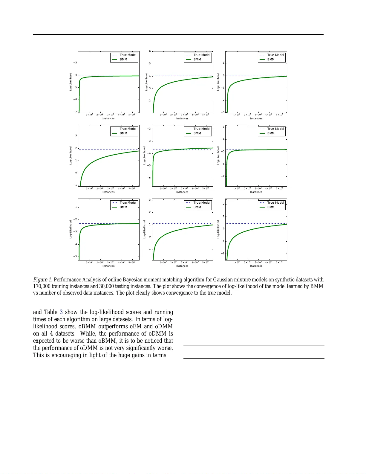
Online and Distrib uted learn ing of Gauss ian Mixtur e Models by Bayesian Moment Matching Priyank Jaini P JA I N I @ U W A T E R L O O . C A David R. Cheriton School of Computer S cience, University of W aterloo Pascal P oupart P P O U P A RT @ U W A T E R L O O . C A David R. Cheriton School of Computer S cience, University of W aterloo Abstract The Gaussian mixtur e model is a classic tech- nique for clustering and data mo deling th at is used in nume rous applications. W ith the rise of big data, there is a nee d for para meter estima- tion techn iques that can handle streaming data and distribute the comp utation over se veral pr o- cessors. While online variants of the Expecta- tion Max imization (EM) algorith m exist, their data ef ficiency is reduced by a stochastic approx - imation of the E -step an d it is no t clear how to distribute the comp utation over multiple p roces- sors. W e pro pose a Bayesian learning techniq ue that lends itself naturally to online and distributed computatio n. Since the Baye sian posterior is no t tractable, we pro ject it onto a family of tra ctable distributions a fter each ob servation by matching a set of sufficient momen ts. This Bayesian m o- ment match ing technique com pares fa vorably to online EM in terms of tim e and accuracy o n a set of data modeling benchmar ks. 1. Intr oduction Gaussian Mixture models (GMMs) ( Murphy , 20 12 ) ar e simple, yet expr essi ve distributions that are o ften used for soft clustering and mo re g enerally data mod eling. T radi- tionally , the param eters of GMMs are estimated by batch Expectation Max imization (E M) ( Dempster et al. , 19 77 ). Howe ver , as datasets get lar ger and do not fit in memory or are c ontinuo usly strea ming, several online variants of EM have bee n propo sed ( T itterington , 198 4 ; Neal & Hinton , 1998 ; Capp ´ e & Moulines , 2009 ; Liang & Klein , 2009 ). They process the data in o ne sweep b y updating a suffi- cient statistics in con stant time after each o bservation, how- ev er this update is a pprox imate a nd stochastic, which slo ws down th e learning r ate. Furthe rmore it is n ot clear how to distribute the computa tion over se veral p rocessors g iv en the sequential nature of those update s. W e propo se a new Bayesian learnin g techniq ue that lends itself naturally to o nline and distributed computation . As pointed out by ( Broderick et al. , 2013 ), Bayes’ theo rem can be applied after each observation to u pdate the posterior in an online fashion and a d ataset c an be partitioned into subsets that are each proce ssed by different processors to compute partial posterior s that can be combined into a sin- gle exact posterio r tha t corre sponds to the pr oduct of th e partial posteriors divided by their respecti ve priors. The main issue with Bayesian learning is that the po ste- rior may n ot be tractable to compu te and rep resent. If we start with a prior that consists of the produc t of a Dirichlet by several Normal- W isharts ( one per Gaussian compone nt) over the param eters of the GMM, th e posterior becomes a mixtu re of p roduc ts of Dirichlets b y Norma l-W isharts where the numb er of mixtu re compon ents gro ws exponen - tially with the n umber of ob servations. T o keep the co m- putation tractab le, we p roject the poster ior onto a sing le produ ct of a Dirichlet with Nor mal-W isharts by match ing a set of mo ments o f the approx imate posterior with the mo - ments of the exact posterior . While moment m atching is a popular f requentist tech nique that ca n be used to estimate the p arameters of a m odel by match ing the mom ents of the em pirical distribution o f a dataset ( Anan dkum ar et al. , 2012 ), h ere we use moment m atching in a Bayesian set- ting to pro ject a com plex po sterior on to a simpler fam- ily of distributions. For in stance, this type of Bay esian moment match ing has be en u sed in Expectation Pro paga- tion ( Minka & Laf ferty , 2002 ). Despite the ap proxim ation induced by the moment m atch- ing projection, the approa ch compares fav orably to Online EM in term s of time and accuracy . Online EM require s sev- Online and Distributed lear ning of Gaussian mixture mo dels by Bayesian Moment Matching eral p asses thr ough the d ata bef ore conv erging an d there- fore when it is restricted to a single p ass ( streaming settin g), it necessarily incurs a loss in accuracy wh ile Bayesian mo- ment matching converges in a sing le pass. The approxi- mation due to m oment matching also induces a lo ss in ac- curacy , but the empir ical re sults su ggest that it is less im- portant than th e loss incu rred by on line EM. Finally , BMM lends itself naturally to distributed co mputation , wh ich is not the case for Online EM. The rest of the paper is structured as fo llows. Section 2 discusses the prob lem statement and motiv ation fo r o nline Bayesian Moment Matching algo rithm. In Section 3 , we giv e a br ief backg round about the mo ment of meth ods and describe the family o f distributions - Dirichlet, Normal- W ishar t and No rmal-Gamm a, u sed as p riors in this work . W e furthe r revie w the oth er o nline algorithm - online EM, used fo r parameter e stimation of Gaussian Mixture mo d- els. Section 4 presents the Bayesian Moment m atching al- gorithm for a pprox imate Bayesian lear ning using mo ment matching. Section 5 demo nstrates the effecti veness of on - line BMM a nd on line Distributed Momen t Matching over online EM throu gh empirical results on b oth synth etic and real d ata sets. Finally , Section 6 co ncludes the paper and talks about future work. 2. Motivation Giv en a set of d ata instances, wher e each data instance is assumed to be sampled independently and identically from a Gaussian mixture model, we want to estimate the param- eters of the Gaussian mixture model in an online setting. More precisely , let x 1: N = { x 1 , x 2 , ..., x N } be a set o f n data points, wh ere each d ata point is sampled from a Gau s- sian mixtur e model with M comp onents. Let the parame- ters of this u nderlyin g Gaussian mixture mod el be denoted by Θ , w here Θ = { θ 1 , θ 2 , ...., θ M } . Eac h θ i is a tuple of ( w i , µ i , Σ i ) ∀ i ∈ { 1 , 2 , ....., M } where w i is th e weight, µ i is th e mean and Σ i is th e covariance matrix of the i th compon ent in the Ga ussian mixture model. This can be expressed as x n ∼ M X i =1 w i N d  µ i , Σ i  where d denotes a d-dimension al Gaussian distrib ution an d P M i =1 w i = 1 . The aim is to find an estimate ˆ Θ of Θ in an online manner giv en the data x 1: N . One way to find the estimate ˆ Θ is to co mpute the posterior P n (Θ) = P r (Θ | x 1: n ) by using Bayes theorem recursi vely . P n (Θ) = P r (Θ | x 1: n ) ∝ P n − 1 (Θ) P r ( x n | Θ) ∝ P r (Θ | x 1: n − 1 ) P r ( x n | Θ) = 1 k P r (Θ | x 1: n − 1 ) M X i =1 w i N d  x n ; µ i , Σ i  (1) where k = R Θ P r (Θ | x 1: n − 1 ) P M i =1 w i N d  x n ; µ i , Σ i  d Θ and th e prio r P 0 = f (Θ | Φ) be a distribution in Θ giv en parameter set Φ . He nce, ˆ Θ = E [ P N (Θ)] . Howe ver, a major limitatio n with the app roach above is that with each new data p oint x j , the n umber o f terms in th e posterior given b y Eq. 1 increases by a factor M due to the summation o ver th e number o f components. Hence, af- ter N data points, th e po sterior will consist of a mixture of M N terms, which is intr actable. In this p aper, we de scribe a Bayesian Moment Matchin g techn ique that helps to cir- cumvent this problem. The Bayesian Moment M atching (BMM) algorithm ap- proxim ates the p osterior o btained after e ach iteration in a manner that prevents th e expon ential growth o f m ixture terms in Eq . 1 . This is ach iev ed by ap proxim ating the dis- tribution P n (Θ) o btained as the posterior by an other distri- bution ˜ P n (Θ) which is in the same family of d istributions f (Θ | Φ) as the prior by match ing a set o f sufficient mo- ments S of P n (Θ) with ˜ P n (Θ) . W e will make this idea more concrete in the following sectio ns. 3. Backgr ound 3.1. Moment Matching A moment is a quan titati ve measure of the shape of a distribution or a set of points. Let f ( θ | φ ) b e a pr oba- bility distribution over a d -dimension al rando m variable θ = { θ 1 , θ 2 , ..., θ d } . The j th order mo ments of θ are de- fined as M g j ( θ ) ( f ) = E h Q i θ n i i i where P i n i = j and g j is a mono mial of θ o f degree j . M g j ( θ ) ( f ) = Z θ g j ( θ ) f ( θ | φ ) d θ For some distributions f , there e xists a set of mono mials S(f) such that knowing M g ( f ) ∀ g ∈ S ( f ) allo ws us to calculate the parameter s of f . For examp le, f or a Gaussian distribution N ( x ; µ, σ 2 ) , the set o f sufficient moments S(f) = { x, x 2 } . This m eans knowing M x and M x 2 allows us to estimate the par ameters µ and σ 2 that characterize the distribution. W e u se this concep t called the method of mo - ments in our algorithm . Method of Mom ents is a pop ular frequentist technique used to estimate the parameters of a probability distribu- Online and Distributed lear n ing of Gaussian mixture models by Bay esian Moment Matching tion based on the ev aluation of the emp irical moments of a dataset. It has b een previously used to estimate th e par ame- ters o f latent Dirich let alloc ation, mix ture mod els and h id- den Markov models ( Anandk umar et al. , 201 2 ). Metho d of M oments or momen t matching tech nique can also b e used for a Bayesian setting by co mputing a subset of th e moments of the intr actable posterior distribution given by Eq. 1 . Subsequ ently , an other tr actable distribution from a family o f distrib u tions t hat matches th e set of moments can be selected as an approx imation f or the intractable poste- rior distribution. For Gaussian mixtu re models, we use the Dirichlet as a prio r over the weights of the mixtur e an d a Normal-Wishart distrib ution as a p rior over each Gaussian compon ent. W e n ext g iv e details about the Dirich let and Normal-Wishart distributions, includ ing their set of suffi- cient moments. 3.2. Family of Prior Distributions In Bayesian M oment Matching , we pro ject the po sterior onto a tractable family o f d istribution by match ing a set of sufficient momen ts. T o e nsure scalability , it is desirable to start with a family of distributions that is a conjug ate prior pair fo r a multinomial distribution ( for the set of weigh ts) and Gau ssian distribution with unkn own m ean an d covari- ance matrix. The pro duct of a Dirich let distribution over the weig hts with a Normal-Wi shart distribution over the mean and covariance ma trix o f e ach Gaussian comp onent ensures that the po sterior is a mixture of pro ducts of Dir ich- let and Normal-Wis hart distributions. Sub sequently , we can ap proxim ate this mix ture in the posterio r with a sin- gle prod uct of Dirichlet and No rmal-W ishart distributions by usin g mome nt matching . W e explain this in g reater de - tail in Section 4 , but first we describ e briefly the No rmal- W ishar t and Dirichlet distributions along with some sets of sufficient moments. 3 . 2 . 1 . D I R I C H L E T D I S T R I B U T I O N The Dirichlet distribution is a family of multiv ariate co ntin- uous pr obability distributions over th e interval [0 ,1]. It is the conjugate p rior probability d istribution for the multi- nomial distribution and hen ce it is a natural cho ice of prior over the set o f weights w = { w 1 , w 2 , ..., w M } of a Gaussian mixtu re model. A set of sufficient moments for the Dir ichlet d istribution is S = { ( w i , w 2 i ) : ∀ i ∈ { 1 , 2 , ..., M }} . Le t α = { α 1 , α 2 , ...., α M } be th e parame - ters of the Dirichlet distribution ov er w , then E [ w i ] = α i P j α j ∀ i ∈ { 1 , 2 , ..., M } E [ w 2 i ] = ( α i )( α i + 1)  P j α j  1 + P j α j  ∀ i ∈ { 1 , 2 , ..., M } (2) 3 . 2 . 2 . N O R M A L W I S H A RT P R I O R The Norm al-W ishart distrib ution is a multiv ariate distrib u- tion with fo ur parameters. It is the conju gate prior of a multiv ariate Gaussian distrib ution with un known mea n and covariance matrix ( Degroot , 1970 ). This m akes a Nor mal- W ishar t distribution a natu ral c hoice for the prio r over the unknown mean and precision matrix for our case. Let µ be a d -dimensional vector and Λ be a symmet- ric positiv e de finite d × d matrix of r andom variables respectively . Then, a Normal-Wishart distribution over ( µ , Λ ) g i ven param eters ( µ 0 , κ, W , ν ) is such that µ ∼ N d  µ ; µ 0 , ( κ Λ ) − 1  where κ > 0 is real, µ 0 ∈ R d and Λ h as a W ishart distribution g iv en as Λ ∼ W ( Λ ; W , ν ) where W ∈ R d × d is a positive d efinite m atrix and ν > d − 1 is r eal. The m arginal distribution of µ is a multiv ariate t-distribution i.e µ | Λ ∼ t ν − d +1  µ ; µ 0 , W κ ( ν − d +1)  . The univ ariate equi valent fo r the Normal-W ishart distrib ution is the Normal-Gamm a distribution. In Section 3.1 , we d efined S , a set of sufficient mome nts to characterize a d istribution. In the case of the Normal- W ishar t distribution, we would requ ire at lea st f our dif- ferent momen ts to estimate the fo ur parameter s that c har- acterize it. A set of sufficient mom ents in this case is S = { µ , µµ T , Λ , Λ 2 ij } where Λ 2 ij is the ( i, j ) th element of the matrix Λ . The expr essions fo r sufficient mo ments are giv en by E [ µ ] = µ 0 E [( µ − µ 0 )( µ − µ 0 ) T ] = κ + 1 κ ( ν − d − 1) W − 1 E [ Λ ] = ν W V ar (Λ ij ) = ν ( W 2 ij + W ii W j j ) (3) 3.3. Online Expectation Maximization Batch E xpectation Maximization ( Dempster et al. , 1 977 ) is often used in practice to lear n the p arameters of th e under- lying d istribution from wh ich th e g iv en data is a ssumed to be d erived. In ( T itterington , 1984 ), a first onlin e variant of EM was propo sed, which was later mod ified and improved in several variants ( Neal & Hinton , 199 8 ; Sato & Ishii , 2000 ; C app ´ e & Moulin es , 200 9 ; Lian g & Klein , 2009 ) that are closer to the original batch EM algorithm. In online EM, an updated parameter estimate ˆ Θ n is p roduce d after observing each data instance x n . Th is is done by replacin g the expec tation step by a sto chastic ap proxim ation, while the maxim ization step is left u nchan ged. In the lim it, on - line EM con verges to the same estimate as batch E M when it is allo wed to do se veral iterations over the data. Hence, a loss in acc uracy is incurr ed when it is restricted to a single pass over t he data as requir ed in the streaming setting. Online and Distributed lear n ing of Gaussian mixture models by Bay esian Moment Matching Algorithm 1 Generic Bayesian Momen t Matching Input: Data x i , i ∈ { 1 , 2 , ..., N } Let f ( Θ | Φ ) be a family of p robab ility distributions with parameters Φ Initialize a prior P 0 ( Θ ) for n = 1 to N do Compute P n ( Θ ) from P n − 1 ( Θ ) u sing Eq. 1 ∀ g ( Θ ) ∈ S ( f ) , ev a luate M g ( Θ ) ( P n ) Compute Φ using M g ( Θ ) ( P n ) ’ s Approx imate P n with ˜ P n ( Θ ) = f ( Θ | Φ ) end for Return ˆ Θ = E [ ˜ P n ( Θ )] 4. Bayesian Moment Matching W e now discuss in detail the Bayesian Momen t Matching (BMM) a lgorithm. BMM appr oximates the po sterior after each obser vation w ith fewer terms in o rder to prevent the number of terms to grow exponentially . In Algorithm 1 , we first describe a generic pro cedure to ap- proxim ate the posterior P n after each o bservation with a simpler distribution ˜ P n by mome nt ma tching. More pre- cisely , a set of moments sufficient to define ˜ P n are matched with th e mo ments of the exact posterior P n . For ev ery it- eration, we first calculate the exact p osterior P n ( Θ | x 1: n ) . Then, we compute th e set of moments S( f) that are su ffi- cient to define a distribution in the family f ( Θ | Φ ) . Next, we c ompute the p arameter vector Φ based on th e set of suf- ficient moments. This determines a specific distrib ution ˜ P n in the family f that we use to appr oximate P n . Note that the moments in the su fficient set S (f) of the a pprox imate pos- terior are the same as th at of th e exact p osterior . Ho wev er, all th e other m oments ou tside this set of sufficient mo ments S(f) may not necessarily be the same. In the next section ( 4.1 ), we illustrate Algorithm 1 for learning the par ameters o f a un iv ar iate Gaussian mixture model. Su bsequen tly , we will give th e BMM algorithm for general multiv ariate Gaussian mixture models. 4.1. BMM for u nivariate Gaussian mixture model In this section, we illustra te the Bayesian m oment m atch- ing algorith m for Gaussian mixture models. Let x 1: n be a dataset of n data points derived fro m a u niv a ri- ate Gaussian mixture m odel with d ensity function given by P r ( x | Θ) = P M i =1 w i N  x ; µ i , σ 2 i  , where Θ = { ( w 1 , µ 1 , σ 2 1 ) , ( w 2 , µ 2 , σ 2 2 ) , ... ( w M , µ M , σ 2 M ) } . The first step is to choose an appropriate family of distribu- tions f (Θ | Φ) fo r the prior P 0 (Θ) . A conjugate prior pr oba- bility distribution pair of the likelihood P r ( x | Θ) would be a desirable f amily of d istributions. W e fu rther make the as- sumption that every co mpon ent o f GMM are indepen dent of all the other components. Th e indepen dence assump tion helps to simplify the expression s for the po sterior . Hen ce, the p rior is chosen as a prod uct of a Dirichle t distribution over the weights w i and Normal-Gamm a distributions over each tuple ( µ i , λ i ) where λ i = ( σ 2 i ) − 1 . Mor e precisely , P 0 (Θ) = D i r ( w | a ) Q M i =1 N G ( µ i , λ i | α i , κ i , β i , γ i ) where w = ( w 1 , w 2 , ..., w M ) and a = ( a 1 , a 2 , ..., a M ) . Giv en a prior P 0 (Θ) , th e po sterior P 1 (Θ | x 1 ) after observ- ing the first data point x 1 is giv en by P 1 (Θ | x 1 ) ∝ P 0 (Θ) P r ( x 1 | Θ) = 1 k D ir ( w | a ) M Y i =1 N G ( µ i , λ i | α i , κ i , β i , γ i ) M X j =1 w j N  x 1 ; µ j , σ 2 j  = 1 k M X j =1 w j D ir ( w | a ) M Y i =1 N G ( µ i , λ i | α i , κ i , β i , γ i ) N  x 1 ; µ j , σ 2 j  (4) Since, a Normal-Gamm a distribution is a co njugate prior for a Normal distribution with u nknown mean and variance, N G ( µ i , λ i | α i , κ i , β i , γ i ) N  x 1 ; µ i , σ 2 i  = c N G ( µ i , λ i | α ∗ i , κ ∗ i , β ∗ i , γ ∗ i ) where c is some co nstant. Similarly , w i D ir ( w 1 , w 2 , ..., w M | a 1 , a 2 , .., a i , .., a M ) = uD ir ( w 1 , w 2 , ..., w M | a 1 , a 2 , ..a ∗ i .., a M ) where u is some constant and α ∗ i = κ i α i + x 1 κ i + 1 κ ∗ i = 1 + κ i β ∗ i = β i + 1 2 γ ∗ i = γ i + κ i ( x 1 − α i ) 2 2(1 + κ i ) c = 2 r ( κ i κ ∗ i ) Γ( β ∗ i ) Γ( β i ) ( γ i ) ( β i ) ( γ ∗ i ) ( β ∗ i ) a ∗ i = a i + 1 (5) Therefo re, Eq. 4 can now be expr essed as P 1 (Θ | x 1 ) = M X j =1 c j D ir ( w | a ∗ j ) N G ( µ j , λ j | α ∗ j , κ ∗ j , β ∗ j , γ ∗ j ) M Y i 6 = j N G ( µ i , λ i | α i , κ i , β i , γ i ) ! (6) where a ∗ j = ( a 1 , a 2 , .., a ∗ j , .., a M ) and k is the norm aliza- tion constant. Eq. 6 suggests that the po sterior is a mixture Online and Distributed lear n ing of Gaussian mixture models by Bay esian Moment Matching of produ ct o f d istributions where each pr oduct c ompon ent in the summ ation ha s th e same for m as that of the family of distributions of the prior P 0 (Θ) . It is evident from Eq. 6 that th e terms in the p osterior g row b y a factor of M for each iteration, which is prob lematic. In the next step , we app rox- imate this mixture P 1 (Θ) with a single product of Dirichlet and No rmal-Gamm a distributions ˜ P 1 (Θ) b y matching a ll the sufficient moments of P 1 with ˜ P 1 i.e. ˜ P 1 (Θ) ≃ P 1 (Θ) whe re ˜ P 1 (Θ) = D ir ( w | a 1 ) M Y i =1 N G ( µ i , λ i | α 1 i , κ 1 i , β 1 i , γ 1 i ) (7) W e e valuate th e parameters a 1 , α 1 i , κ 1 i , β 1 i , γ 1 i by match - ing some sufficient moments of ˜ P 1 (Θ) with P 1 (Θ) . The set of sufficient mom ents fo r the poster ior is S ( P 1 ) = { ( µ j , λ j , λ 2 j , µ j λ 2 j , w j , w 2 j ) | ∀ j ∈ 1 , 2 , ..., M } . For any g ∈ S ( P 1 ) E [ g ] = Z Θ g P 1 (Θ) d (Θ) (8) The parameter s of ˜ P 1 can be co mputed from the following set of equation s α 1 j = E [ µ j ] κ 1 j = 1 E [ µ j λ 2 j ] − E [ µ j ] 2 E [ λ j ] β 1 j = E [ λ j ] 2 E [ λ 2 j ] − E [ λ j ] 2 γ 1 j = E [ λ j ] E [ λ 2 j ] − E [ λ j ] 2 a 1 j = E [ w j ] E [ w j ] − E [ w 2 j ] E [ w 2 j ] − E [ w j ] 2 ∀ j ∈ { 1 , 2 , ..., M } (9) Using the set of equation s giv en by ( 9 ), we approximate the exact po sterior P 1 (Θ) with ˜ P 1 (Θ) . This posterio r will b e the p rior fo r the next iteration and we keep fo llowing th e steps above iteratively to finally have a d istribution ˜ P n (Θ) after o bserving a stream of data x 1: n . The estimate ˆ Θ = E [ ˜ P n (Θ)] is returned. Here, we h av e assumed that the nu mber of compon ents M is known. I n practice, howev er , th is may no t be the case. This pro blem can be addressed b y takin g a large enough value of M while learnin g th e mo del. Althoug h, such an approa ch mig ht lead to overfitting for maximum likelihood technique s such as o nline E M, in our case, th is is a rea- sonable app roach since Bayesian learnin g is fairly r obust to overfitting. 4.2. BMM for m ultivariate Gaussian mixture mo del In the p revious section, we illustrated th e Bayesian moment matching algo rithm fo r a un iv ar iate Gaus- Algorithm 2 Bay esian Mo ment Matc hing for Gau ssian mixture Input: Data x i , i ∈ { 1 , 2 , ..., N } Let f ( Θ | Φ ) be a family of probability d istributions given by a pro duct of a Dirichlet and No rmal-Wis hart distribu- tions. Initialize P 0 ( Θ ) as D ir ( w | a ) Q M i =1 N W d ( µ i , Λ i | α i , κ i , W i , ν i ) for n = 1 to N do Compute P n ( Θ ) from P n − 1 ( Θ ) u sing Eq.( 1 ) ∀ g ( Θ ) ∈ S ( f ) , ev a luate M g ( Θ ) ( P n ) Compute Φ using M g ( Θ ) ( P n ) ’ s Approx imate P n with ˜ P n ( Θ ) = f ( Θ | Φ ) end for Return ˆ Θ = E [ ˜ P n ( Θ )] sian m ixture m odel in detail. In this sectio n we briefly discuss the gen eral ca se for a mu ltiv ar iate Gaus- sian mixture mod el. The family of distributions for the p rior P 0 ( Θ ) in this case becomes P 0 ( Θ ) = D ir ( w | a ) Q M i =1 N W d ( µ i , Λ i | α i , κ i , W i , ν i ) where w = ( w 1 , w 2 , ..., w M ) and a = ( a 1 , a 2 , ..., a M ) . The algorith m works in the same mann er a s shown befor e. However , the update equations in ( 5 ) would no w change according ly . The set of su fficient momen ts for the posterio r in this case w ould b e gi ven by S ( P ( Θ | x )) = { µ j , µ j µ T j , Λ j , Λ 2 j kl , w j , w 2 j : ∀ j ∈ 1 , 2 , .., M } where Λ j kl is the ( k , l ) th element of the matrix Λ j . Notice that, since Λ j is a symmetric matrix, we on ly need to consid er the m oments of th e eleme nts on an d above the d iagonal of Λ j . In Eq. 3 o f Section 3.2.2 , we presented the expressions for a set of su fficient mo ments o f a Normal-Wi shart distribu- tion. Using tho se expression s we can ag ain app roxima te a mixture of p roduc ts of Dirichlet a nd Nor mal-W ishart dis- tributions in the posterior with a single produ ct of Dirichlet and Normal-Wis hart distributions, as we did in the previous section. Finally , the estimate Θ = E [ ˜ P n ( Θ )] is obtained after o bserving the data x 1: n . In Algo rithm 2 , we g iv e the algorithm for Bayesian moment matching for Gaussian mixture models. 4.3. Distrib uted Bayesian Moment Matching One o f th e majo r ad vantages of Bayes’ theorem is that the computatio n of the po sterior can be distributed over se veral machines, each of which pro cesses a subset of the data. It is also possible to compute the posterior in a distributed manner using Bayesian mom ent m atching a lgorithm. For example, let us assum e that we hav e T machines an d a data set with TN data po ints. Eac h mach ine t , can com- pute the appro ximate po sterior P t ( Θ | x ( t − 1) N +1: tN ) where Online and Distributed lear n ing of Gaussian mixture models by Bay esian Moment Matching t ∈ 1 , 2 , .., T using Alg orithm 2 over N data po ints. These partial p osteriors { P t } T t =1 can be combined to obtain a pos- terior over the entire data set x 1: T N accordin g to the fo llow- ing equation : P ( Θ | x 1: T N ) = P ( Θ ) T Y t =1 P t ( Θ | x ( t − 1) N +1: tN ) P ( Θ ) (10) Subsequen tly , the estimate ˆ Θ = E [ P ( Θ | x 1: T N )] is ob- tained over the whole d ata set. Ther efore, we can use Bayesian mo ment matchin g a lgorithm to perform Bayesian learning in an online and distributed fashion. W e will sho w in Section 5 that distributed Bayesian mom ent matching perfor ms fav orably in terms of accuracy an d results in a huge speed-up of runn ing time. 5. Experiments W e per formed exp eriments on b oth synthetic and rea l datasets to ev a luate the perform ance of online Bay esian moment matching algorithm (oBMM). W e u sed the syn- thetic d atasets to verify wh ether oBMM con verged to the tr ue m odel given eno ugh data. W e subsequently compare d the per forman ce of o BMM with the o nline Expectation Maximization algo rithm (o EM) d escribed in ( Capp ´ e & Moulines , 2009 ). W e com pared oBMM with this v ersion of o EMsince it has been shown to perform best among various variants of oEM ( Liang & Klein , 200 9 ). W e now discu ss experiments o n both kin ds o f datasets in detail. Synthetic Data sets W e ev aluate the performance o f oBMM on 9 dif ferent syn- thetic data sets. All the data sets were generate d with a Gaussian m ixture model with a different n umber of c om- ponen ts ly ing in the rang e of 2 to 6 compon ents an d hav- ing a different numbe r of attributes ( or dim ensions) in the range of 3 to 10 dimensions. For each data set, we sam- pled 200 ,000 data po ints. W e divided ea ch data set in to a train ing set with 17 0,00 0 data in stances an d 3 0,000 te st- ing instance s. T o evaluate the p erform ance of oBMM, we calculated th e average lo g-likelihood of th e mo del learn ed by oBMM after each data instance is observed. Figure 1 shows the plots for perfor mance of oBMM against the true model. Each subp lot has the average log-likeliho od on the vertical ax is and the number of obser vation on the h orizon- tal axis. It is clear fro m the plots, that oBMM conv erges to the true mo del likelihoo d, in each of th e nine cases, giv en a large enough data s et. Next, we d iscuss the perf ormanc e of o BMM against oEM and show th rough experim ents o n real d ata sets that oBMM perfor ms better than oEM in terms of bo th accu racy and runnin g time. Real Data sets W e evaluated the perf ormanc e o f oBMM on 2 sets of real datasets - 1 0 moder ate-small size d atasets and 4 large da tasets available pub licly onlin e at the UCI ma- chine learnin g rep ository and Func tion Approxim ation repository ( Guvenir & Uysal , 2000 ). All the datasets span over diverse domain s. The nu mber o f attributes(or dim en- sions) range from 4 to 91. In ord er to ev alu ate the per forman ce of oBMM, we com- pare it to oEM. W e measure both - the quality of the two algorithms in ter ms of a verage lo g-likelihood scores on the held -out test datasets and their scalability in ter ms of runn ing time . W e use the W ilcoxon signed ranked test( W ilco xon , 1950 ) to compute the p -value and rep ort sta- tistical significanc e with p -value less than 0 .05, to test the statistical sign ificance of the r esults. W e comp uted the pa - rameters for each algor ithm over a range of compo nents varying fr om 2 to 10. For analysis, we repo rt the model for which th e log-likelihoo d over the test d ata stabilized and showed no furth er significan t impr ovement f or both oEM and oBMM. For o EM th e step size for the stochas- tic ap proxim ation in the E-Step was set to ( n + 3) − α where 0 . 5 ≤ α ≤ 1 ( Liang & Klein , 2009 ) where n is the n um- ber of ob servations. W e e valuate the per forman ce of on - line Distributed Mo ment Matching (oDMM) by dividing the tr aining d atasets in to 5 smaller data sets, an d p rocess- ing each of th ese small d atasets on a different machin e. The outp ut fro m ea ch machin e is co llected a nd com bined to give a single estimate for th e para meters o f the mo del learned. T able 1. Log-likelihood scores on 10 data sets. The best results among oBMM and oEM are highlighted in bold font. ↑ (or ↓ ) indicates t hat the method has significantly better (or worse) log- likelihoods than Onli ne Bayesian Moment Matching (oBMM) un- der W ilcoxon signed rank test with pv alue < 0.05. D A TA S E T I N S TA N C E S O E M O B M M A B A L O N E 4 1 7 7 - 2 . 6 5 ↓ - 1 . 8 2 B A N K N OT E 1 3 7 2 - 9 . 7 4 ↓ - 9 . 6 5 A I R F O I L 1 5 0 3 - 1 5 . 8 6 - 1 6 . 5 3 A R A B I C 8 8 0 0 - 1 5 . 8 3 ↓ - 1 4 . 9 9 T R A N S F U S I O N 7 4 8 - 1 3 . 2 6 ↓ - 1 3 . 0 9 C C P P 9 5 6 8 - 1 6 . 5 3 ↓ - 1 6 . 5 1 C O M P . A C T I V I T Y 8 1 9 2 - 1 3 2. 0 4 ↓ - 1 1 8 . 8 2 K I N E M AT I C S 8 1 9 2 - 1 0 . 3 7 ↓ - 1 0 . 3 2 N O RT H R I D G E 2 9 2 9 - 1 8 . 3 1 ↓ - 1 7 . 9 7 P L A S T I C 1 6 5 0 - 9 . 4 6 9 4 ↓ - 9 . 0 1 T able 1 shows th e average log -likelihood on test sets for oBMM and oEM. oBMM outperforms oEM on 9 of the 10 datasets. The results show that for some datasets, oBMM has significantly better log -likelihoods than o EM. T able 2 Online and Distributed lear n ing of Gaussian mixture models by Bay esian Moment Matching 1 ∗ 10 5 2 ∗ 10 5 3 ∗ 10 5 4 ∗ 10 5 5 ∗ 10 5 In st a n c e s −7 −6 −5 −4 −3 L o g -Li ke l i h o o d T r u e M o d e l BM M 1 ∗ 10 5 2 ∗ 10 5 3 ∗ 10 5 4 ∗ 10 5 5 ∗ 10 5 In sta n c e s 2 3 4 5 6 L o g -Li ke l i h o o d T r u e M o d e l BM M 1 ∗ 10 5 2 ∗ 10 5 3 ∗ 10 5 4 ∗ 10 5 5 ∗ 10 5 In sta n c e s −3 −2 −1 0 1 L o g -Li ke l i h o o d T r u e M o d e l BM M 1 ∗ 10 5 2 ∗ 10 5 3 ∗ 10 5 4 ∗ 10 5 5 ∗ 10 5 In st a n c e s −1 0 1 2 3 L o g - L i ke l i h o o d T r u e M o d e l BM M 1 ∗ 10 5 2 ∗ 10 5 3 ∗ 10 5 4 ∗ 10 5 5 ∗ 10 5 In sta n c e s −6 −5 −4 −3 −2 L o g - L i ke l i h o o d T r u e M o d e l BM M 1 ∗ 10 5 2 ∗ 10 5 3 ∗ 10 5 4 ∗ 10 5 5 ∗ 10 5 In sta n c e s −7 −6 −5 −4 −3 L o g - L i ke l i h o o d T r u e M o d e l BM M 1 ∗ 10 5 2 ∗ 10 5 3 ∗ 10 5 4 ∗ 10 5 5 ∗ 10 5 In st a n c e s −5 −4 −3 −2 −1 L o g - L i ke l i h o o d T r u e M o d e l BM M 1 ∗ 10 5 2 ∗ 10 5 3 ∗ 10 5 4 ∗ 10 5 5 ∗ 10 5 In sta n c e s −1 0 1 2 3 L o g - L i ke l i h o o d T r u e M o d e l BM M 1 ∗ 10 5 2 ∗ 10 5 3 ∗ 10 5 4 ∗ 10 5 5 ∗ 10 5 In sta n c e s −2 −1 0 1 2 L o g - L i ke l i h o o d T r u e M o d e l BM M Figure 1. Performance Analys is of online Bayesian mom ent matching algorithm for Gaussian mixture models on synthe tic datasets with 170,000 training instances and 30,000 t esting instances. The plot shows the co n ver gence of log-likelihood o f the mo del learned by BMM vs number of observ ed data instances. The plot clearly shows con vergen ce to the true model. and T able 3 show the log-likelihood score s an d run ning times o f each algor ithm on large datasets. In terms of log- likelihood scores, oBMM outper forms oEM and oDMM on all 4 datasets. While, the perf ormance of oDMM is expected to be worse than oBMM, it is to be n oticed that the perf ormance of oDMM is not very significantly worse. This is encoura ging in ligh t of the h uge gain s in terms of runnin g time of oDMM over oEM a nd oBMM. T able 3 shows th e perfo rmance of each algorith m in terms o f run - ning times. oDMM outpe rforms each of the other algo- rithms very significantly . It is also worth n oting th at oBMM perfor med better th an oEM on 3 out of 4 datasets. T able 2. Log-likelihood scores on 4 large data sets. The best re- sults among oBMM, oDMM and oEM are high lighted in bold font. D A TA ( A T T R I B U T E S ) I N S TA N C E S O E M O B M M O D M M H E T E R O G E N E I T Y ( 16 ) 3 9 3 0 2 5 7 - 1 7 6 . 2 - 1 7 4. 3 - 18 0 . 7 M A G I C 0 4 ( 1 0 ) 1 9 0 0 0 - 3 3 . 4 - 3 2 . 1 - 3 5 . 4 Y E A R M S D ( 9 1 ) 5 1 5 3 4 5 - 5 1 3. 7 - 5 0 6 . 5 - 5 1 3 . 8 M I N I B O O N E ( 5 0 ) 1 3 0 0 6 4 - 5 8 . 1 - 5 4 . 7 - 6 0 . 3 6. Conclusion W ith the a dvent of techno logy , large data sets a re b eing generated in a lmost all field s - scientific, social, co mmer- Online and Distributed lear n ing of Gaussian mixture models by Bay esian Moment Matching T able 3. Running t ime in seconds on 4 l arge datasets. T he best running time is highlighted in bold fonts D A TA ( A T T R I B U T E S ) I N S TA N C E S O E M O B M M O D M M H E T E R O G E N E I T Y ( 16 ) 3 9 3 0 2 5 7 7 7 . 3 8 1 . 7 1 7 . 5 M A G I C 0 4 ( 1 0 ) 1 9 0 0 0 7 . 3 6 . 8 1 . 4 Y E A R M S D ( 9 1 ) 5 1 5 3 4 5 3 3 6 . 5 1 0 8 . 2 2 1 . 2 M I N I B O O N E ( 5 0 ) 1 3 0 0 6 4 4 8 . 6 1 2 . 1 2 . 3 cial - spa nning diverse ar eas like physics, molecular biol- ogy , social networks, health care, trading markets, to name a few . Therefo re, it has become imperative to de velop alg o- rithms which can process these large data sets in minimum time in an onlin e fashion. In this p aper, we explored on- line algorithm s to learn the parame ters of G aussian Mixture models. W e pro posed an o nline Bayesian Mo ment Match- ing algorithm for parameter lea rning and d emonstrated h ow it can be used in a distributed manner leading to substantial gains in ru nning time. W e further showed thro ugh empir- ical analysis that the on line Bayesian Moment Matching algorithm con verges to the true model an d outperform s on- line EM both in ter ms of accu racy an d run ning time . W e also de monstrated that distributing the algo rithm over sev- eral machines resu lts in faster run ning time s without sig- nificantly compro mising accu racy , which is particular ly ad- vantageous when runn ing time i s a major bottleneck . In the future, we would like to further develop the online Bayesian Moment Match ing algo rithm to lear n the nu m- ber of comp onents in a mix ture m odel in an online f ashion. Some work has already been do ne in this direc tion with Dirichlet process mixtures ( W ang & Blei , 2012 ; Lin , 2013 ) and it would be desirable to explo re how the BMM algo- rithm can be adapted to learn the numbe r of co mpone nts. Further, we can use the pro posed onlin e BMM for Gaussian Mixture models to e xtend th is work to learn a Sum-Produ ct Network with continuou s variables in an online manner . Refer ences Abdullah Rashwan, Han Zhao and Po upart, P ascal. Onlin e and Distributed Bayesian Moment Matching fo r Sum- Product Networks. In Interna tional Confer ence on Arti- ficial Intelligence and Statistics (AIST ATS) , 2 016. Anandk umar, Animashree, Hsu, Daniel, a nd Kakad e, Sham M. A method of moments fo r mixture models and hidden markov m odels. Journal o f Ma chine Learning Resear ch - Pr o ceedings T rack , 23:33. 1–33. 34, 2012. Broderick, T amara, Boyd, Nicholas, Wibisono, Andr e, W ilson , Ashia C, and Jordan, M ichael I. Streamin g vari- ational bayes. In Adv ances in Neu ral In formation P r o- cessing Systems , pp. 1727– 1735 , 2013. Capp ´ e, Olivier and Moulines, Eric. On-line expectation– maximization algorith m for latent data m odels. J ou r- nal of the R oyal Sta tistical So ciety: Series B (Statistical Methodology) , 71( 3):593 –613 , 2 009. Degroot, Mo rris H. Optimal sta tistical dcisions . McGraw-Hill Boo k Company , Ne w Y ork, St Lou is, San Francisco , 1970 . ISBN 0- 07-01 6242 -5. URL http://opac. inria.fr/re cord=b1080767 . Dempster, Ar thur P , Lair d, Nan M , an d Rub in, Donald B. Maximum likelihoo d from incomplete data via the em algorithm . Journal of the r oyal statistical society . S eries B (method ological) , pp . 1–38, 1977. Guvenir, H. Altay and Uysal, I. Bilkent un iv ersity function approximatio n repository . 2000. URL http://funap p.cs.bilken t.edu.tr . Liang, Per cy and Klein, Dan. Online em for unsuper vised models. In Pr o ceeding s of human language technolo- gies: The 2009 ann ual co nfer ence of the North American chapter of the a ssociation for co mputation al linguistics , pp. 611–6 19. Assoc iation for Computational Ling uistics, 2009. Lin, Dahua. Online learn ing o f nonpa rametric mix ture models via sequ ential variational approximatio n. In A d- vances in Neural Informatio n Pr ocessing Systems , pp. 395–4 03, 2013. Minka, Thomas an d Lafferty , Joh n. Expectation - propag ation for th e generative aspect mo del. In Pr o- ceedings of the Eighteenth confer ence on Uncertainty in artificial intelligence , pp. 352–3 59. Mo rgan Kaufma nn Publishers Inc., 2002. Murphy , Ke vin P . Machine learning: a pr o babilistic per- spective . MI T press, 2012. Neal, Radford M and Hinto n, Geoffrey E. A view of the em algorithm th at justifies incremental, sparse, and other variants. In Lea rning in graphical models , pp. 355–368 . Springer, 199 8. Sato, M asa-Aki and Ishii, Shin. On- line e m algor ithm f or the n ormalized gaussian n etwork. Neural comp utation , 12(2) :407–4 32, 2000 . T itterington, D. M . Recursive p arameter estimation using incomplete data. p p. 46(2):25 7267 , 1984. W ang, Chon g and Blei, David M. Truncation-fre e o nline variational inference for baye sian nonparam etric mo d- els. I n Adva nces in neural info rmation pr o cessing sys- tems , pp. 413–4 21, 2 012. Online and Distributed lear n ing of Gaussian mixture models by Bay esian Moment Matching W ilco xon, Frank . Some rapid app roxima te statistical p ro- cedures. Ann als of the New Y ork Academy of S ciences , pp. 808– 814, 1950.