Bayesian Reinforcement Learning: A Survey

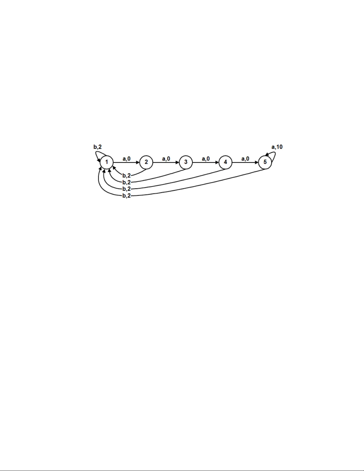
F oundations and T rends R  in Machine Learning V ol. 8, No. 5-6 (2015) 359–492 c  2015 M. Ghav amzadeh, S. Mannor, J. Pineau, and A. T amar DOI: 10.1561/2200000049 Ba yesian Reinfo rcement Lea rning: A Survey Mohammad Gha v amzadeh A dob e Researc h & INRIA mohammad.gha v amzadeh@inria.fr Shie Mannor T ec hnion shie@ee.tec hnion.ac.il Jo elle Pineau McGill Univ ersit y jpineau@cs.mcgill.ca A viv T amar Univ ersit y of California, Berk eley a vivt@b erk eley .edu Contents 1 Intro duction 3 2 T echnical Background 11 2.1 Multi-Armed Bandits . . . . . . . . . . . . . . . . . . . . 11 2.2 Ma rk ov Decision Pro cesses . . . . . . . . . . . . . . . . . 14 2.3 P a rtially Observable Ma rk ov Decision Pro cesses . . . . . . 18 2.4 Reinfo rcement Lea rning . . . . . . . . . . . . . . . . . . . 20 2.5 Ba y esian Lea rning . . . . . . . . . . . . . . . . . . . . . . 22 3 Ba y esian Bandits 29 3.1 Classical Results . . . . . . . . . . . . . . . . . . . . . . . 30 3.2 Ba y es-UCB . . . . . . . . . . . . . . . . . . . . . . . . . . 33 3.3 Thompson Sampling . . . . . . . . . . . . . . . . . . . . . 33 4 Mo del-based Bay esian Reinforcement Lea rning 41 4.1 Mo dels and Rep resentations . . . . . . . . . . . . . . . . . 41 4.2 Explo ration/Exploitation Dilemma . . . . . . . . . . . . . 45 4.3 Oﬄine V alue App ro ximation . . . . . . . . . . . . . . . . 46 4.4 Online nea r-my opic value app ro ximation . . . . . . . . . . 48 4.5 Online T ree Search App ro ximation . . . . . . . . . . . . . 50 4.6 Metho ds with Explo ration Bonus to A chieve P A C Gua rantees 56 4.7 Extensions to Unkno wn Rew a rds . . . . . . . . . . . . . . 64 iii iv 4.8 Extensions to Continuous MDPs . . . . . . . . . . . . . . 67 4.9 Extensions to P a rtially Observable MDPs . . . . . . . . . 69 4.10 Extensions to Other Prio rs and Structured MDPs . . . . . 72 5 Mo del-free Bay esian Reinforcement Lea rning 75 5.1 V alue F unction Algo rithms . . . . . . . . . . . . . . . . . 75 5.2 Ba y esian P olicy Gradient . . . . . . . . . . . . . . . . . . 86 5.3 Ba y esian A cto r-Critic . . . . . . . . . . . . . . . . . . . . 95 6 Risk-a w a re Ba y esian Reinfo rcement Lea rning 101 7 BRL Extensions 109 7.1 P A C-Bay es Model Selection . . . . . . . . . . . . . . . . . 109 7.2 Ba y esian Inverse Reinfo rcement Lea rning . . . . . . . . . . 110 7.3 Ba y esian Multi-agent Reinfo rcement Lea rning . . . . . . . 113 7.4 Ba y esian Multi-T ask Reinforcement Lea rning . . . . . . . . 113 8 Outlo ok 117 A ckno wledgements 121 App endices 123 A Index of Symb ols 125 B Discussion on GPTD Assumptions on the Noise Pro cess 129 References 131 Abstract Ba y esian metho ds for mac hine learning ha v e b een widely inv estigated, yielding principled metho ds for incorp orating prior information in to inference algorithms. In this surv ey , w e pro vide an in-depth review of the role of Ba y esian metho ds for the reinforcemen t learning (RL) paradigm. The ma jor incen tiv es for incorp orating Ba y esian reasoning in RL are: 1) it pro vides an elegant approach to action-selection (explo- ration/exploitation) as a function of the uncertain t y in learning; and 2) it pro vides a mac hinery to incorp orate prior knowledge into the al- gorithms. W e ﬁrst discuss mo dels and metho ds for Bay esian inference in the simple single-step Bandit mo del. W e then review the extensive recen t literature on Ba y esian metho ds for mo del-based RL, where prior information can b e expressed on the parameters of the Marko v mo del. W e also present Ba y esian metho ds for mo del-free RL, where priors are expressed ov er the v alue function or p olicy class. The ob jectiv e of the pap er is to provide a comprehensiv e survey on Bay esian RL algorithms and their theoretical and empirical prop erties. M. Gha v amzadeh, S. Mannor, J. Pineau, and A. T amar. Bayesian R einfor c ement L earning: A Survey . F oundations and T rends R  in Mac hine Learning, v ol. 8, no. 5-6, pp. 359–492, 2015. DOI: 10.1561/2200000049. 1 Intro duction A large num ber of problems in science and engineering, from rob otics to game pla ying, tutoring systems, resource managemen t, ﬁnancial p ort- folio management, medical treatmen t design and b ey ond, can b e c har- acterized as sequen tial decision-making under uncertaint y . Many inter- esting sequen tial decision-making tasks can b e formulated as reinforce- men t learning (RL) problems [Bertsekas and T sitsiklis, 1996, Sutton and Barto, 1998]. In an RL problem, an agen t in teracts with a dy- namic, sto chastic, and incompletely kno wn en vironmen t, with the goal of ﬁnding an action-selection strategy , or p olicy , that optimizes some long-term p erformance measure. One of the k ey features of RL is the fo cus on learning a con trol p olicy to optimize the c hoice of actions ov er sev eral time steps. This is usually learned from sequences of data. In contrast to sup ervised learn- ing metho ds that deal with indep endently and identically distributed (i.i.d.) samples from the domain, the RL agen t learns from the sam- ples that are collected from the tra jectories generated by its sequential in teraction with the system. Another imp ortant asp ect is the eﬀect of the agent’s p olicy on the data collection; diﬀeren t p olicies naturally yield diﬀerent distributions of sampled tra jectories, and th us, impact- 3 4 CHAPTER 1. INTRODUCTION ing what can b e learned from the data. T raditionally , RL algorithms ha v e b een categorized as b eing either mo del-b ase d or mo del-fr e e . In the former category , the agen t uses the collected data to ﬁrst build a mo d el of the domain’s dynamics and then uses this mo del to optimize its p olicy . In the latter case, the agen t di- rectly learns an optimal (or go o d) action-selection strategy from the collected data. There is some evidence that the ﬁrst metho d provides b etter results with less data [Atk eson and Santamaria, 1997], and the second metho d may be more eﬃcien t in cases where the solution space (e.g., p olicy space) exhibits more regularity than the underlying dy- namics, though there is some disagreemen t ab out this,. A major challenge in RL is in identifying go o d data collection strate- gies, that eﬀectively balance b etw een the need to explore the space of all p ossible policies, and the desire to fo cus data collection to w ards tra- jectories that yield b etter outcome (e.g., greater c hance of reaching a goal, or minimizing a cost function). This is kno wn as the explor ation- exploitation tradeoﬀ. This c hallenge arises in b oth model-based and mo del-free RL algorithms. Ba y esian reinforcement learning (BRL) is an approac h to RL that lev erages metho ds from Bay esian inference to incorp orate information in to the learning pro cess. It assumes that the designer of the system can express prior information ab out the problem in a probabilistic distri- bution, and that new information can b e incorp orated using standard rules of Ba y esian inference. The information can b e enco ded and up- dated using a parametric representation of the system dynamics, in the case of mo del-based RL, or of the solution space, in the case of mo del-free RL. A ma jor adv antage of the BRL approach is that it provides a p rin- cipled wa y to tac kle the exploration-exploitation problem. Indeed, the Ba y esian posterior naturally captures the full state of knowledge, sub- ject to the chosen parametric representation, and th us, the agen t can select actions that maximize the expected gain with respect to this information state. Another ma jor adv an tage of BRL is that it implicitly facilitates reg- ularization. By assuming a prior on the v alue function, the parameters 5 deﬁning a p olicy , or the mo del parameters, we a v oid the trap of letting a few data p oints steer us a w a y from the true parameters. On the other hand, ha ving a prior precludes o v erly rapid con v ergence. The role of the prior is therefore to soften the eﬀect of sampling a ﬁnite dataset, eﬀectiv ely leading to regularization. W e note that regularization in RL has b een addressed for the v alue function [F arahmand et al., 2008b] and for p olicies [F arahmand et al., 2008a]. A ma jor issue with these regularization schemes is that it is not clear how to select the regu- larization co eﬃcient. Moreov er, it is not clear why an optimal v alue function (or a p olicy) should b elong to some pre-deﬁned set. Y et another adv antage of adopting a Bay esian view in RL is the principled Bay esian approac h for handling parameter uncertaint y . Cur- ren t frequen tist approac hes for dealing with mo delling errors in sequen- tial decision making are either v ery conserv ative, or computationally infeasible [Nilim and El Ghaoui, 2005]. By explicitly mo delling the dis- tribution ov er unkno wn system parameters, Bay esian metho ds oﬀer a promising approac h for solving this diﬃcult problem. Of course, sev eral c hallenges arise in applying Ba y esian methods to the RL paradigm. First, there is the challenge of selecting the correct represen tation for expressing prior information in an y given domain. Second, deﬁning the decision-making pro cess ov er the information state is t ypically computationally more demanding than directly considering the natural state representation. Nonetheless, a large arra y of mo dels and algorithms ha v e b een prop osed for the BRL framew ork, leverag- ing a v ariet y of structural assumptions and approximations to provide feasible solutions. The main ob jectiv e of this paper is to pro vide a comprehensiv e surv ey on BRL algorithms and their theoretical and empirical prop er- ties. In Chapter 2, we pro vide a review of the main mathematical con- cepts and techniques used throughout this pap er. Chapter 3 surveys the Ba y esian learning metho ds for the case of single-step decision-making, using the b andit framework. This section serves b oth as an exp osition of the p otential of BRL in a simpler setting that is w ell understo o d, but is also of indep enden t in terest, as bandits hav e widespread applications. The main results presen ted here are of a theoretical nature, outlin- 6 CHAPTER 1. INTRODUCTION ing kno wn p erformance b ounds for the regret minimization criteria. Chapter 4 reviews existing metho ds for mo del-b ase d BRL, where the p osterior is expressed ov er parameters of the system dynamics mo del. Chapter 5 fo cuses on BRL metho ds that do not explicitly learn a mo del of the system, but rather the p osterior is expressed ov er the solution space. Chapter 6 fo cuses on a particular adv antage of BRL in dealing with risk due to parameter-uncertain t y , and surv eys sev eral approac hes for incorp orating such risk into the decision-making pro cess. Finally , Chapter 7 discusses v arious extensions of BRL for sp ecial classes of problems (P A C-Ba y es mo del selection, inv erse RL, m ulti-agen t RL, and m ulti-task RL). Figure 1.1 outlines the v arious BRL approaches cov- ered throughout the pap er. An Example Domain W e presen t an illustrativ e domain suitable to be solv ed using the BRL tec hniques surv ey ed in this pap er. This running example will b e used throughout the pap er to elucidate the diﬀerence b etw een the v arious BRL approac hes and to clarify v arious BRL concepts. Example 1.1 (The Online Shop) . In the online shop domain, a retailer aims to maximize proﬁt by sequentially suggesting pro ducts to online shopping customers. F ormally , the domain is characterized by the fol- lo wing mo del: • A set of p ossible customer states, X . States can represent intrinsic features of the customer such as gender and age, but also dynamic quan tities suc h as the items in his shopping cart, or his willingness to shop; • A set of p ossible pro duct suggestions and advertisemen ts, A ; • A probability k ernel, P , deﬁned b elow. An episo de in the online shop domain b egins at time t = 0 , when a customer with features x 0 ∈ X en ters the online shop. Then, a se- quen tial in teraction betw een the customer and the online shop b egins, where at each step t = 0 , 1 , 2 , . . . , an adv ertisemen t a t ∈ A is shown 7 ! !"#"$%&'$($%&)*#$+*,,%+'& ! -../0.& & ! -(1%'"(#&23& ! 456&7%8+"'9)& & ! !*+:(+;&'%(+)7& ! -(1%'"(#&'<(+'%&'(=<,"#>& ! ?@23& ! -!AB& ! -+(#)7C(#;CD*8#;&'%(+)7& ! -E@F3& & ! -5AA& ! -.-& ! 4-G-& ! -50/& & ! H3/2& ! H3AEGAE& ! -(1%'"(#&I8(;+($8+%& ! /:*&-(1%'"(#&=*;%,'&J*+&& %'9=(9#>&$7%&<*,")1&>+(;"%#$& & ! H3/2&K&-(1%'"(#&<*,")1&>+(;"%#$& "#$%&'()) * +,-)./) 01%,2!3#(,%) "45)*+,-)6/) 01%,2!78,,) "45)*+,-)9/) ) ) ) ) " #:,();<") = >1?@(1$)(#?@2&$A) ) ) ) B C&$,)D#2E,)#@@81F&?#G1$) ) ) B $2&$,)$,#8!?:1@&-)D#2E,)#@@81F&?#G1$) ) ) B $2&$,)'8,,)(,#8->)#@@81F&?#G1$) ) ) ) ) ) ) H F@218#G1$)31$E()#@@81F&?#G1$) ) ) ) ) I #2E,)7E$-G1$)#2A1() ) ) J 12&-:)A8#%&,$')#2A1() ) ) ) K -'18!<8&G-)#2A1( )) ) "#:,(&#$) 45) 4&(L)KM#8,)) "45)*+,-)N/) "&#()D#8&#$-,)#@@81F&?#G1$) J,8-,$G2,)-8&',8&1$) 0&$!?#F)-8&',8&1$) J,8-,$G2,)?,#(E8,()-8&',8&#) Figure 1.1: Overview of the Ba y esian RL approaches cov ered in this survey . 8 CHAPTER 1. INTRODUCTION to the customer, and follo wing that the customer mak es a decision to either (i) add a product to his shopping cart; (ii) not buy the pro duct, but contin ue to shop; (iii) stop shopping and chec k out. F ollo wing the customers decision, his state changes to x t +1 (reﬂecting the change in the shopping cart, willingness to con tin ue shopping, etc.). W e assume that this c hange is captured b y a probabilit y k ernel P ( x t +1 | x t , a t ) . When the customer decides to chec k out, the episo de ends, and a proﬁt is obtained according to the items he had added to his cart. The goal is to ﬁnd a product suggestion p olicy , x → a ∈ A , that maximizes the exp ected total proﬁt. When the probabilities of customer resp onses P are known in ad- v ance, calculating an optimal p olicy for the online shop domain is basi- cally a planning problem, whic h may b e solved using traditional meth- o ds for resource allo cation [Po w ell, 2011]. A more challenging, but real- istic, scenario is when P is not completely kno wn b eforehand, but has to b e le arne d while in teracting with customers. The BRL framew ork emplo ys Bayesian metho ds for learning P , and for learning an optimal pro duct suggestion p olicy . There are several adv an tages for c ho osing a Ba y esian approac h for the online shop domain. First, it is lik ely that some prior knowledge ab out P is av ailable. F or example, once a customer adds a pro duct of a particular brand to his cart, it is likely that he prefers additional pro ducts of the same brand o v er those of a diﬀerent one. T aking into accoun t such kno wledge is natural in the Bay esian metho d, by virtue of the prior distribution o ver P . As w e shall see, the Ba yesian ap- proac h also naturally extends to more general forms of structur e in the problem. A second adv an tage concerns what is known as the exploitation– explor ation dilemma: should the decision-maker display only the most proﬁtable pro duct suggestions according to his curren t knowledge ab out P , or rather take exploratory actions that ma y turn out to b e less proﬁtable, but provide useful information for future decisions? The Ba y esian metho d oﬀers a principled approach to dealing with this dif- ﬁcult problem by explicitly quan tifying the v alue of exploration, made p ossible b y main taining a distribution o v er P . 9 The v arious parameter conﬁgurations in the online shop domain lead to the diﬀeren t learning problems survey ed in this pap er. In par- ticular: • F or a single-step interaction, i.e., when the episo de terminates after a single prod uct suggestion, the problem is captured by the m ulti-armed bandit mo del of Chapter 3. • F or small-scale problems, i.e., a small n um b er of pro ducts and customer types, P may b e learnt explicitly . This is the mo del- based approac h of Chapter 4. • F or large problems, a near-optimal p olicy may b e obtained with- out representing P explicitly . This is the mo del-free approac h of Chapter 5. • When the customer state is not fully observed b y the decision- mak er, we require mo dels that incorp orate partial observ ability; see §2.3 and §4.9. Throughout the pap er, w e revisit the online shop domain, and sp ec- ify explicit conﬁgurations that are relev ant to the survey ed methods. 2 T echnical Background In this section we pro vide a brief ov erview of the main concepts and in tro duce the notations used throughout the pap er. W e b egin with a quic k review of the primary mathematical to ols and algorithms lever- aged in the latter sections to deﬁne BRL mo dels and algorithms. 2.1 Multi-Armed Bandits As was previously mentioned, a k ey challenge in sequential decision- making under uncertain t y is the exploration/exploitation dilemma: the tradeoﬀ b et w een either taking actions that are most rewarding accord- ing to the curren t state of kno wledge, or taking exploratory actions, whic h ma y b e less immediately rewarding, but ma y lead to b etter in- formed decisions in the future. The sto chastic multi-arme d b andit (MAB) problem is p erhaps the simplest mo del of the exploration/exploitation tradeoﬀ. Originally for- m ulated as the problem of a gam bler choosing b etw een diﬀerent slot mac hines in a casino (‘one armed bandits’), the sto c hastic MAB model features a decision-mak er that sequen tially c ho oses actions a t ∈ A , and observ es random outcomes Y t ( a t ) ∈ Y at discrete time steps 11 12 CHAPTER 2. TECHNICAL BACK GROUND t = 1 , 2 , 3 , . . . . A known function r : Y → R asso ciates the random outcome to a rew ard, whic h the agen t seeks to maximize. The out- comes { Y t ( a ) } are dra wn i.i.d. ov er time from an unknown probability distribution P ( ·| a ) ∈ P ( Y ) , where P ( Y ) denotes the set of probability distributions on (Borel) subsets of Y (see Bub ec k and Cesa-Bianchi [2012] for reference). Mo del 1 (Sto c hastic K -Armed Bandit) Deﬁne a K -MAB to b e a tuple hA , Y , P , r i where • A is the set of actions (arms), and |A| = K , • Y is the set of p ossible outcomes, • P ( ·| a ) ∈ P ( Y ) is the outcome probability , conditioned on action a ∈ A b eing tak en, • r ( Y ) ∈ R represents the reward obtained when outcome Y ∈ Y is observ ed. A rule that prescribes to the agent whic h actions to select, or p olicy , is deﬁned as a mapping from past observ ations to a distribution ov er the set of actions. Since the probability distributions are initially unkno wn, the decision-mak er faces a tradeoﬀ b etw een exploitation, i.e., selecting the arm she b elieves is optimal, or making exploratory actions to gather more information ab out the true probabilities. F ormally , this tradeoﬀ is captured b y the notion of r e gr et : Deﬁnition 2.1 (Regret) . Let a ∗ ∈ arg max a ∈A E y ∼ P ( ·| a )  r ( y )  denote the optimal arm. The T -p erio d regret of the sequence of actions a 1 , . . . , a T is the random v ariable Regret ( T ) = T X t =1 h r  Y t ( a ∗ )  − r  Y t ( a t )  i . T ypically , MAB algorithms fo cus on the exp e cte d r e gr et , E  Regret ( T )  , and provide p olicies that are guaran teed to k eep it small in some sense. As an illustration of the MAB mo del, let us revisit the online shop example. Example 2.1 (Online shop – bandit setting) . Recall the online shop do- main of Example 1.1. In the MAB setting, there is no state information 2.1. MUL TI-ARMED BANDITS 13 ab out the customers, i.e., X = ∅ . In addition, each interaction lasts a single time step, after which the customer chec ks out, and a proﬁt is obtained according to his purchasing decision. The regret minimization problem corresp onds to determining whic h sequence of advertisemen ts a 1 , . . . , a T to show to a stream of T incoming customers, suc h that the total rev en ue is close to that whic h w ould ha v e b een obtained with the optimal adv ertisemen t stream. In some cases, the decision-maker may hav e access to some addi- tional information that is imp ortant for making decisions, but is not captured in the MAB mo del. F or example, in the online shop domain of Example 2.1, it is lik ely that some information ab out the customer, such as his age or origin, is a v ailable. The c ontextual b andit model (a.k.a. asso ciativ e bandits, or bandits with side information) is an extension of the MAB mo del that tak es suc h information in to accoun t. The decision-making pro cess in the contextual bandit model is sim- ilar to the MAB case. Ho w ev er, at eac h time step t , the decision maker ﬁrst observes a context s t ∈ S , drawn i.i.d. o v er time from a probabilit y distribution P S ( · ) ∈ P ( S ) , where P ( S ) denotes the set of probability distributions on (Borel) subsets of S . The decision-maker then chooses an action a t ∈ A and observ es a random outcome Y t ( a t , s t ) ∈ Y , which no w dep ends b oth on the context and the action. The outcomes { Y t ( a ) } are drawn i.i.d. ov er time from an unknown probability distribution P ( ·| a, s ) ∈ P ( Y ) , where P ( Y ) denotes the set of probabilit y distribu- tions on (Borel) subsets of Y . Mo del 2 (Con textual Bandit) Deﬁne a contextual bandit to b e a tuple hS , A , Y , P S , P , r i where • S is the set of con texts, • A is the set of actions (arms), • Y is the set of p ossible outcomes, • P S ( · ) ∈ P ( S ) is the con text probabilit y , • P ( ·| a, s ) ∈ P ( Y ) is the outcome probability , conditioned on action a ∈ A b eing tak en when the con text is s ∈ S , • r ( Y ) ∈ R represents the reward obtained when outcome Y ∈ Y is observ ed. 14 CHAPTER 2. TECHNICAL BACK GROUND The Marko v decision pro cess mo del, as presented in the following section, ma y be seen as an extension of the con textual bandit model to a se quential decision-making mo del, in whic h the con text is no longer i.i.d., but ma y c hange o v er time according to the selected actions. 2.2 Ma rk ov Decision Pro cesses The Marko v Decision Pro cess (MDP) is a framew ork for sequen tial decision-making in Marko vian dynamical systems [Bellman, 1957, Put- erman, 1994]. It can b e seen as an extension of the MAB framew ork b y adding the notion of a system state , that may dynamically change according to the performed actions and aﬀects the outcomes of the system. Mo del 3 (Marko v Decision Pro cess) Deﬁne an MDP M to b e a tuple hS , A , P , P 0 , q i where • S is the set of states, • A is the set of actions, • P ( ·| s, a ) ∈ P ( S ) is the probabilit y distribution o v er next states, con- ditioned on action a b eing tak en in state s , • P 0 ∈ P ( S ) is the probabilit y distribution according to whic h the ini- tial state is selected, • R ( s, a ) ∼ q ( ·| s, a ) ∈ P ( R ) is a random v ariable represen ting the re- w ard obtained when action a is tak en in state s . Let P ( S ) , P ( A ) , and P ( R ) b e the set of probabilit y distributions on (Borel) subsets of S , A , and R resp ectively . 1 W e assume that P , P 0 and q are stationary . Throughout the pap er, w e use upp er-case and lo w er-case letters to refer to random v ariables and the v alues taken b y random v ariables, resp ectively . F or example, R ( s, a ) is the random v ariable of the immediate reward, and r ( s, a ) is one p ossible realization of this random v ariable. W e denote the exp ected v alue of R ( s, a ) , as ¯ r ( s, a ) = R r q ( dr | s, a ) . Assumption A1 (MDP Regularity) W e assume that the random immediate rew ards are b ounded by R max and the expected immediate 1 R is the set of real num b ers. 2.2. MARKOV DECISION PROCESSES 15 rew ards are b ounded b y ¯ R max . Note that ¯ R max ≤ R max . A rule according to whic h the agen t selects its actions at eac h p ossible state, or p olicy , is deﬁned as a mapping from past observ ations to a distribution ov er the set of actions. A p olicy is called Markov if the distribution dep ends only on the last state of the observ ation sequence. A p olicy is called stationary if it do es not change o v er time. A stationary Mark o v policy µ ( ·| s ) ∈ P ( A ) is a probabilit y distribution o v er the set of actions giv en a state s ∈ S . A p olicy is deterministic if the probabilit y distribution concen trates on a single action for all histories. A deterministic p olicy is identiﬁed b y a mapping from the set of states to the set of actions, i.e., µ : S → A . In the rest of the pap er, we use the term p olicy to refer to stationary Mark o v p olicies. The MDP controlled by a p olicy µ induces a Marko v c hain M µ with rew ard distribution q µ ( ·| s ) = q  · | s, µ ( s )  suc h that R µ ( s ) = R  s, µ ( s )  ∈ q µ ( ·| s ) , transition k ernel P µ ( ·| s ) = P  · | s, µ ( s )  , and sta- tionary distribution o v er states π µ (if it admits one). In a Mark o v c hain M µ , for state-action pairs z = ( s, a ) ∈ Z = S × A , we de- ﬁne the transition densit y and the initial (state-action) density as P µ ( z 0 | z ) = P ( s 0 | s, a ) µ ( a 0 | s 0 ) and P µ 0 ( z 0 ) = P 0 ( s 0 ) µ ( a 0 | s 0 ) , resp ectively . W e generically use ξ = { z 0 , z 1 , . . . , z T } ∈ Ξ , T ∈ { 0 , 1 , . . . , ∞} , to de- note a path (or trajectory) generated by this Marko v chain. The prob- abilit y (densit y) of suc h a path is giv en b y Pr( ξ | µ ) = P µ 0 ( z 0 ) T Y t =1 P µ ( z t | z t − 1 ) . W e deﬁne the (p ossibly discoun ted, γ ∈ [0 , 1] ) return of a path as a function ρ : Ξ → R , ρ ( ξ ) = P T t =0 γ t R ( z t ) . F or eac h path ξ , its (dis- coun ted) return, ρ ( ξ ) , is a random v ariable with the exp ected v alue ¯ ρ ( ξ ) = P T t =0 γ t ¯ r ( z t ) . 2 Here, γ ∈ [0 , 1] is a discoun t factor that de- termines the exp onential dev aluation rate of dela yed rew ards. 3 The 2 When there is no randomness in the rew ards, i.e., r ( s, a ) = ¯ r ( s, a ) , then ρ ( ξ ) = ¯ ρ ( ξ ) . 3 When γ = 1 , the p olicy must b e prop er, i.e., guaranteed to terminate, see [Put- erman, 1994] or [Bertsekas and T sitsiklis, 1996] for more details. 16 CHAPTER 2. TECHNICAL BACK GROUND exp ected return of a p olicy µ is deﬁned b y η ( µ ) = E  ρ ( ξ )  = Z Ξ ¯ ρ ( ξ ) Pr( ξ | µ ) dξ . (2.1) The exp ectation is ov er all p ossible tra jectories generated by p olicy µ and all p ossible rew ards collected in them. Similarly , for a given p olicy µ , w e can deﬁne the (discounted) return of a state s , D µ ( s ) , as the sum of (discounted) rewards that the agen t encoun ters when it starts in state s and follo ws p olicy µ afterw ards D µ ( s ) = ∞ X t =0 γ t R ( Z t ) | Z 0 =  s, µ ( ·| s )  , with S t +1 ∼ P µ ( ·| S t ) . (2.2) The exp ected v alue of D µ is called the v alue function of p olicy µ V µ ( s ) = E  D µ ( s )  = E " ∞ X t =0 γ t R ( Z t )      Z 0 =  s, µ ( ·| s )  # . (2.3) Closely related to v alue function is the action-v alue function of a p olicy , the total exp ected (discounted) rew ard observ ed by the agent when it starts in state s , tak es action a , and then executes p olicy µ Q µ ( z ) = E  D µ ( z )  = E " ∞ X t =0 γ t R ( Z t )      Z 0 = z # , where similarly to D µ ( s ) , D µ ( z ) is the sum of (discounted) rewards that the agen t encoun ters when it starts in state s , takes action a , and follo ws p olicy µ afterwards. It is easy to see that for any p olicy µ , the functions V µ and Q µ are b ounded b y ¯ R max / (1 − γ ) . W e ma y write the v alue of a state s under a p olicy µ in terms of its immediate reward and the v alues of its successor states under µ as V µ ( s ) = R µ ( s ) + γ Z S P µ ( s 0 | s ) V µ ( s 0 ) ds 0 , (2.4) whic h is called the Bel lman e quation for V µ . Giv en an MDP , the goal is to ﬁnd a p olicy that attains the b est p ossible v alues, V ∗ ( s ) = sup µ V µ ( s ) , for all states s ∈ S . The function V ∗ is called the optimal v alue function. A p olicy is optimal (denoted b y µ ∗ ) if it attains the optimal v alues at all the states, i.e., V µ ∗ ( s ) = V ∗ ( s ) 2.2. MARKOV DECISION PROCESSES 17 for all s ∈ S . In order to characterize optimal p olicies it is useful to deﬁne the optimal action-v alue function Q ∗ ( z ) = sup µ Q µ ( z ) . (2.5) F urther, we say that a deterministic p olicy µ is gr e e dy with resp ect to an action-v alue function Q , if for all s ∈ S and a ∈ A , µ ( s ) ∈ arg max a ∈A Q ( s, a ) . Greedy p olicies are imp ortan t b ecause an y greedy p olicy with resp ect to Q ∗ is optimal. Similar to the v alue function of a p olicy (Eq. 2.4), the optimal v alue function of a state s ma y be written in terms of the optimal v alues of its successor states as V ∗ ( s ) = max a ∈A  R ( s, a ) + γ Z S P ( s 0 | s, a ) V ∗ ( s 0 ) ds 0  , (2.6) whic h is called the Bel lman optimality e quation . Note that, similar to Eqs. 2.4 and 2.6, we may deﬁne the Bellman equation and the Bellman optimalit y equation for action-v alue function. It is important to note that almost all metho ds for ﬁnding the optimal solution of an MDP are based on tw o dynamic pr o gr amming (DP) algorithms: value iter ation and p olicy iter ation . V alue iteration (VI) begins with a v alue function V 0 and at each iteration i , generates a new v alue function by applying Eq. 2.6 to the curren t v alue function, i.e., V ∗ i ( s ) = max a ∈A  R ( s, a ) + γ Z S P ( s 0 | s, a ) V ∗ i − 1 ( s 0 ) ds 0  , ∀ s ∈ S . P olicy iteration (PI) starts with an initial p olicy . A t eac h iteration, it ev aluates the v alue function of the current p olicy , this pro cess is referred to as p olicy evaluation (PE), and then p erforms a p olicy impr ovement step, in whic h a new p olicy is generated as a greedy p olicy with resp ect to the v alue of the curren t p olicy . Iterating the policy ev aluation – p ol- icy impro v emen t pro cess is kno wn to produce a strictly monotonically impro ving sequence of p olicies. If the impro v ed p olicy is the same as the p olicy improv ed upon, then w e are assured that the optimal p olicy has b een found. 18 CHAPTER 2. TECHNICAL BACK GROUND 2.3 P a rtially Observable Mark ov Decision Pro cesses The Partially Observ able Marko v Decision Process (POMDP) is an extension of MDP to the case where the state of the system is not necessarily observ able [Astrom, 1965, Smallw o o d and Sondik, 1973, Kaelbling et al., 1998]. Mo del 4 (P artially Observ able Mark o v Decision Pro cess) De- ﬁne a POMDP M to b e a tuple hS , A , O , P , Ω , P 0 , q i where • S is the set of states, • A is the set of actions, • O is the set of observ ations, • P ( ·| s, a ) ∈ P ( S ) is the probabilit y distribution o v er next states, con- ditioned on action a b eing tak en in state s , • Ω( ·| s, a ) ∈ P ( O ) is the probabilit y distribution ov er p ossible obser- v ations, conditioned on action a being taken to reach state s where the observ ation is p erceived, • P 0 ∈ P ( S ) is the probabilit y distribution according to whic h the ini- tial state is selected, • R ( s, a ) ∼ q ( ·| s, a ) ∈ P ( R ) is a random v ariable represen ting the re- w ard obtained when action a is tak en in state s . All assumptions are similar to MDPs, with the addition that P ( O ) is the set of probabilit y distributions on (Borel) subsets of O , and Ω is stationary . As a motiv ation for the POMDP mo del, w e revisit again the online shop domain. Example 2.2 (Online shop – hidden state setting) . Recall the online shop domain of Example 1.1. In a realistic scenario, some features of the customer, such as its gender or age, migh t not b e visible to the decision maker due to priv acy , or other reasons. In such a case, the MDP mo del, which requires the full state information for making decisions is not suitable. In the POMDP model, only observ able quantities, suc h as the items in the shopping cart, are used for making decisions. Since the state is not directly observ ed, the agent must rely on the recent history of actions and observ ations, { o t +1 , a t , o t , . . . , o 1 , a 0 } 2.3. P AR TIALL Y OBSER V ABLE MARKOV DECISION PROCESSES 19 to infer a distribution ov er states. This b elief (also called information state ) is deﬁned o v er the state probabilit y simplex, b t ∈ ∆ , and can b e calculated recursiv ely as: b t +1 ( s 0 ) = Ω( o t +1 | s 0 , a t ) R S P ( s 0 | s, a t ) b t ( s ) ds R S Ω( o t +1 | s 00 , a t ) R S P ( s 00 | s, a t ) b t ( s ) dsds 00 , (2.7) where the sequence is initialized at b 0 := P 0 and the denominator can b e seen as a simple normalization function. F or con v enience, we sometimes denote the b elief up date (Eq. 2.7) as b t +1 = τ ( b t , a, o ) . In the POMDP framework, the action-selection p olicy is deﬁned as µ : ∆( s ) → A . Thus, solving a POMDP inv olv es ﬁnding the optimal p olicy , µ ∗ , that maximizes the exp ected discounted sum of rewards for all b elief states. This can b e deﬁned using a v ariant of the Bellman equation V ∗ ( b t ) = max a ∈A  Z S R ( s, a ) b t ( s ) ds + γ Z O Pr( o | b t , a ) V ∗  τ ( b t , a, o )  do  . (2.8) The optimal v alue function for a ﬁnite-horizon POMDP can b e sho wn to b e piecewise-linear and con v ex [Smallw o o d and Sondik, 1973, Porta et al., 2006]. In that case, the v alue function V t at any ﬁnite plan- ning horizon t can b e represented by a ﬁnite set of linear segments Γ t = { α 0 , α 1 , . . . , α m } , often called α -vectors (when S is discrete) or α -functions (when S is con tin uous). Each deﬁnes a linear function o v er the b elief state space asso ciated with some action a ∈ A . The v alue of a giv en α i at a b elief b t can b e ev aluated by linear interpolation α i ( b t ) = Z S α i ( s ) b t ( s ) ds. (2.9) The v alue of a b elief state is the maxim um v alue returned by one of the α -functions for this b elief state V ∗ t ( b t ) = max α ∈ Γ t Z S α ( s ) b t ( s ) . (2.10) In that case, the b est action, µ ∗ ( b t ) , is the one asso ciated with the α -v ector that returns the b est v alue. The b elief as deﬁned here can be in terpreted as a state in a particu- lar kind of MDP , often called the b elief-MDP . The main in tuition is that 20 CHAPTER 2. TECHNICAL BACK GROUND for any partially observ able system with kno wn parameters, the b elief is actually fully observ able and computable (for small enough state spaces and is appro ximable for others). Th us, the planning problem is in fact one of planning in an MDP , where the state space corresp onds to the b elief simplex. This do es not lead to an y computational adv an- tage, but conceptually , suggests that known results and metho ds for MDPs can also b e applied to the b elief-MDP . 2.4 Reinfo rcement Lea rning Reinforcemen t learning (RL) [Bertsekas and T sitsiklis, 1996, Sutton and Barto, 1998] is a class of learning pr oblems in whic h an agen t (or controller) interacts with a dynamic, sto chastic, and incompletely kno wn en vironmen t, with the goal of ﬁnding an action-selection strat- egy , or p olicy , to optimize some measure of its long-term performance. The interaction is conv entionally mo deled as an MDP , or if the envi- ronmen t state is not alw a ys completely observ able, as a POMDP [Put- erman, 1994]. No w that we hav e deﬁned the MDP mo del, the next step is to solv e it, i.e., to ﬁnd an optimal p olicy . 4 In some cases, MDPs can b e solved analytically , and in many cases they can b e solved iteratively b y dy- namic or line ar pr o gr amming (e.g., see [Bertsekas and T sitsiklis, 1996]). Ho w ev er, in other cases these metho ds cannot b e applied b ecause ei- ther the state space is to o large, a system mo del is av ailable only as a simulator, or no system mo del is av ailable at all. It is in these cases that RL tec hniques and algorithms ma y b e helpful. Reinforcemen t learning solutions can b e viewed as a broad class of sample-based metho ds for solving MDPs. In place of a mo del, these metho ds use sample tra jectories of the system and the agent in teract- ing, such as could b e obtained from a simulation. It is not un usual in practical applications for such a simulator to b e av ailable when an explicit transition-probability mo del of the sort suitable for use b y dy- namic or linear programming is not [T esauro, 1994, Crites and Barto, 4 It is not p ossible to ﬁnd an optimal p olicy in many practical problems. In such cases, the goal would b e to ﬁnd a reasonably go o d p olicy , i.e., a p olicy with large enough v alue function. 2.4. REINFOR CEMENT LEARNING 21 1998]. Reinforcemen t learning methods can also b e used with no model at all, by obtaining sample tra jectories from direct in teraction with the system [Baxter et al., 1998, K ohl and Stone, 2004, Ng et al., 2004]. Reinforcemen t learning solutions can b e categorized in diﬀeren t w a ys. Belo w w e describe tw o common categorizations that are relev ant to the structure of this pap er. Mo del-based vs. Mo del-free Methods: Reinforcement learning algorithms that explicitly learn a system mo del and use it to solve an MDP are called mo del-b ase d metho ds. Some examples of these metho ds are the Dyna arc hitecture [Sutton, 1991] and prioritized sw eeping [Mo ore and A tk eson, 1993]. Mo del-fr e e metho ds are those that do not explicitly learn a system mo del and only use sample tra jectories obtained b y direct in teraction with the system. These metho ds include p opular algorithms such as Q-learning [W atkins, 1989], SARSA [Rummery and Niranjan, 1994], and LSPI [Lagoudakis and P arr, 2003]. V alue F unction vs. Policy Search Metho ds: An imp ortan t class of RL algorithms are those that ﬁrst ﬁnd the optimal v alue function, and then extract an optimal policy from it. This class of RL algorithms contains value function metho ds, of whic h some well- studied examples include v alue iteration (e.g., [Bertsekas and T sitsiklis, 1996, Sutton and Barto, 1998]), p olicy iteration (e.g., [Bertsekas and T sitsiklis, 1996, Sutton and Barto, 1998]), Q-learning [W atkins, 1989], SARSA [Rummery and Niranjan, 1994], LSPI [Lagoudakis and P arr, 2003], and ﬁtted Q-iteration [Ernst et al., 2005]. An alternative ap- proac h for solving an MDP is to directly searc h in the space of p olicies. These RL algorithms are called p olicy se ar ch metho ds. Since the num- b er of p olicies is exp onential in the size of the state space, one has to resort to meta-heuristic searc h [Mannor et al., 2003] or to lo cal greedy metho ds. An imp ortant class of p olicy searc h metho ds is that of p olicy gr adient algorithms. In these algorithms, the p olicy is taken to b e an arbitrary diﬀerentiable function of a parameter v ector, and the searc h in the p olicy space is directed b y the gradient of a p erformance function 22 CHAPTER 2. TECHNICAL BACK GROUND with respect to the policy parameters (e.g., [Williams, 1992, Marbach, 1998, Baxter and Bartlett, 2001]). There is a third class of RL methods that use p olicy gradien t to searc h in the policy space, and at the same time estimate a v alue function. These algorithms are called actor-critic (e.g., [K onda and T sitsiklis, 2000, Sutton et al., 2000, Bhatnagar et al., 2007, Peters and Schaal, 2008, Bhatnagar et al., 2009]). They can b e though t of as RL analogs of dynamic programming’s p olicy iteration metho d. A ctor-critic metho ds are based on the simultaneous online estimation of the parameters of t w o structures, called the actor and the critic . The actor and the critic corresp ond to conv en tional action- selection p olicy and v alue function, resp ectively . These problems are separable, but are solv ed sim ultaneously to ﬁnd an optimal p olicy . 2.5 Ba y esian Lea rning In Ba y esian learning, w e mak e inference ab out a random v ariable X b y pro ducing a probability distribution for X . Inferences, such as p oint and in terv al estimates, may then b e extracted from this distribution. Let us assume that the random v ariable X is hidden and we can only observ e a related random v ariable Y . Our goal is to infer X from the samples of Y . A simple example is when X is a physical quan tit y and Y is its noisy measurement. Bay esian inference is usually carried out in the follo wing w a y: 1. W e choose a probabilit y density P ( X ) , called the prior distri- bution , that expresses our b eliefs ab out the random v ariable X b efore w e observ e an y data. 2. W e select a statistical mo del P ( Y | X ) that reﬂects our b elief ab out Y given X . This mo del represen ts the statistical dep endence b e- t w een X and Y . 3. W e observ e data Y = y . 4. W e update our belief ab out X by calculating its p osterior distri- bution using Ba y es rule P ( X | Y = y ) = P ( y | X ) P ( X ) R P ( y | X 0 ) P ( X 0 ) dX 0 . 2.5. BA YESIAN LEARNING 23 Assume no w that P ( X ) is parameterized by an unknown vector of parameters θ in some parameter space Θ ; w e denote this as P θ ( X ) . Let X 1 , . . . , X n b e a random i.i.d. sample drawn from P θ ( X ) . In general, up dating the p osterior P θ ( X | Y = y ) is diﬃcult, due to the need to compute the normalizing constant R Θ P ( y | X 0 ) P θ ( X 0 ) d θ . How ever, for the case of c onjugate family distributions, w e can up date the posterior in closed-form by simply up dating the parameters of the distribution. In the next tw o sections, we consider three classes of conjugate distribu- tions: Beta and Diric hlet distributions and Gaussian Pro cesses (GPs). 2.5.1 Beta and Dirichlet Distributions A simple example of a conjugate family is the Beta distribution, whic h is conjugate to the Binomial distribution. Let B eta ( α, β ) b e deﬁned b y the densit y function f ( p | α, β ) ∝ p α − 1 (1 − p ) β − 1 for p ∈ [0 , 1] , and parameters α, β ≥ 0 . Let B inomial ( n, p ) b e deﬁned by the densit y function f ( k | n, p ) ∝ p k (1 − p ) n − k for k ∈ { 0 , 1 , . . . , n } , and parameters p ∈ [0 , 1] and n ∈ N . Consider X ∼ B inomial ( n, p ) with unkno wn probabilit y parameter p , and consider a prior B eta ( α, β ) o v er the un- kno wn v alue of p . Then f ollo wing an observ ation X = x , the p osterior o v er p is also Beta distributed and is deﬁned by B eta ( α + x, β + n − x ) . No w let us consider the multiv ariate extension of this conjugate family . In this case, w e hav e the Multinomial distribution, whose con- jugate is the Dirichlet distribution. Let X ∼ M ul tinomial k ( p, N ) b e a random v ariable with unknown probability distribution p = ( p 1 , . . . , p k ) . The Dirichlet distribution is parameterized by a coun t v ec- tor φ = ( φ 1 , . . . , φ k ) , where φ i ≥ 0 , such that the density of probabilit y distribution p = ( p 1 , . . . , p k ) is deﬁned as f ( p | φ ) ∝ Q k i =1 p φ i − 1 i . The distribution D ir ichl et ( φ 1 , . . . , φ k ) can also be in terpreted as a prior o v er the unknown Multinomial distribution p , suc h that after observ- ing X = n , the p osterior o ver p is also Dirichlet and is deﬁned b y D ir ichlet ( φ 1 + n 1 , . . . , φ k + n k ) . 2.5.2 Gaussian Pro cesses and Gaussian Pro cess Regression A Gaussian pro cess (GP) is an indexed set of jointly Gaussian ran- dom v ariables, i.e., F ( x ) , x ∈ X is a Gaussian pro cess if and only 24 CHAPTER 2. TECHNICAL BACK GROUND if for ev ery ﬁnite set of indices { x 1 , . . . , x T } in the index set X ,  F ( x 1 ) , . . . , F ( x T )  is a v ector-v alued Gaussian random v ariable. The GP F ma y b e thought of as a random v ector if X is ﬁnite, as a ran- dom series if X is countably inﬁnite, and as a random function if X is uncountably inﬁnite. In the last case, eac h instantiation of F is a function f : X → R . F or a giv en x , F ( x ) is a random v ariable, nor- mally distributed jointly with the other comp onents of F . A GP F can b e fully sp eciﬁed b y its mean ¯ f : X → R , ¯ f ( x ) = E [ F ( x )] and co v ariance k : X × X → R , k ( x, x 0 ) = Co v [ F ( x ) , F ( x 0 )] , i.e., F ( · ) ∼ N  ¯ f ( · ) , k ( · , · )  . The k ernel function k ( · , · ) enco des our prior kno wledge concerning the correlations b et w een the comp onents of F at diﬀeren t points. It ma y be thought of as inducing a measure of pro ximit y b et w een the mem bers of X . It can also b e shown that k de- ﬁnes the function space within which the searc h for a solution takes place (see [Schölk opf and Smola, 2002, Sha w e-T aylor and Cristianini, 2004] for more details). No w let us consider the follo wing generativ e mo del: Y ( x ) = H F ( x ) + N ( x ) , (2.11) where H is a general linear transformation, F is an unknown function, x is the input, N is a Gaussian noise and indep enden t of F , and Y is the observ able pro cess, mo deled as a noisy v ersion of H F . The ob jectiv e here is to infer F from samples of Y . Ba y esian learning can be applied to this problem in the follo wing w a y . 1. W e c hoose a prior distribution for F in the form of a GP , F ( · ) ∼ N  ¯ f ( · ) , k ( · , · )  . When F and N are Gaussian and indep endent of each other, the generative mo del of Eq. 2.11 is kno wn as the line ar statistic al mo del [Sc harf, 1991]. 2. The statistical dep endence b etw een F and Y is deﬁned by the mo del-equation (2.11). 3. W e observ e a sample in the form of D T = { ( x t , y t ) } T t =1 . 4. W e calculate the p osterior distribution of F conditioned on the sample D T using the Ba y es rule. Below is the pro cess to calculate this p osterior distribution. 2.5. BA YESIAN LEARNING 25 F ( x 1 ) F ( x 2 ) F ( x T ) Y ( x 1 ) Y ( x 2 ) Y ( x T ) N ( x T ) N ( x 2 ) N ( x 1 ) Figure 2.1: A directed graph illustrating the conditional independencies betw een the laten t F ( x t ) v ariables (bottom row), the noise v ariables N ( x t ) (top row), and the observ able Y ( x t ) v ariables (middle row), in GP regression (when H = I ). All of the F ( x t ) v ariables should b e in terconnected by arro ws (forming a clique), due to the dep endencies introduced by the prior. T o av oid cluttering the diagram, this w as mark ed by the dashed frame surrounding them. Figure 2.1 illustrates the GP regression setting (when H = I ) as a graphical mo del in which arro ws mark the conditional dep endency re- lations b etw een the no des corresp onding to the laten t F ( x t ) and the observ ed Y ( x t ) v ariables. The mo del-equation (2.11) ev aluated at the training samples ma y b e written as Y T = H F T + N T , (2.12) where F T =  F ( x 1 ) , . . . , F ( x T )  > , Y T = ( y 1 , . . . , y T ) > , and N T ∼ N ( 0 , Σ ) . Here [ Σ ] i,j is the measurement noise cov ariance b etw een the i th and j th samples. In the linear statistical mo del, w e then hav e F T ∼ N ( ¯ f , K ) , where ¯ f =  ¯ f ( x 1 ) , . . . , ¯ f ( x T )  > and [ K ] i,j = k ( x i , x j ) is a T × T kernel matrix. Since b oth F T and N T are Gaussian and indep enden t from each other, we hav e Y T ∼ N ( H ¯ f , H K H > + Σ ) . Consider a query p oin t x , w e then ha v e    F ( x ) F T N T    = N         ¯ f ( x ) ¯ f 0    ,    k ( x, x ) k ( x ) > 0 k ( x ) K 0 0 0 Σ         , where k ( x ) =  k ( x 1 , x ) , . . . , k ( x T , x )  > . Using Eq. 2.12, w e ha v e the 26 CHAPTER 2. TECHNICAL BACK GROUND follo wing transformation:    F ( x ) F T Y T    =    1 0 0 0 I 0 0 H I       F ( x ) F T N T    , (2.13) where I is the iden tit y matrix. F rom Eq. 2.13, w e ha v e    F ( x ) F T Y T    = N         ¯ f ( x ) ¯ f H ¯ f    ,    k ( x, x ) k ( x ) > k ( x ) > H > k ( x ) K K H > H k ( x ) H K H K H > + Σ         . Using the Gauss-Mark o v theorem [Scharf, 1991], we kno w that F ( x ) | Y T (or equiv alently F ( x ) |D T ) is Gaussian, and obtain the fol- lo wing expressions for the posterior mean and cov ariance of F ( x ) con- ditioned on the sample D T : E  F ( x ) |D T  = ¯ f ( x ) + k ( x ) > H > ( H K H > + Σ ) − 1 ( y T − H ¯ f ) , Co v  F ( x ) , F ( x 0 ) |D T  = k ( x, x 0 ) − k ( x ) > H > ( H K H > + Σ ) − 1 H k ( x 0 ) , (2.14) where y T = ( y 1 , . . . , y T ) > is one realization of the random vector Y T . It is p ossible to decomp ose th e expressions in Eq. 2.14 into input de- p enden t terms (whic h dep end on x and x 0 ) and terms that only dep end on the training samples, as follo ws: E  F ( x ) |D T  = ¯ f ( x ) + k ( x ) > α , Co v  F ( x ) , F ( x 0 ) |D T  = k ( x, x 0 ) − k ( x ) > C k ( x 0 ) , (2.15) where α = H > ( H K H > + Σ ) − 1 ( y T − H ¯ f ) , C = H > ( H K H > + Σ ) − 1 H . (2.16) F rom Eqs. 2.15 and 2.16, we can conclude that α and C are suﬃcient statistics for the p osterior momen ts. If w e set the transformation H to b e the iden tit y and assume that the noise terms corrupting each sample are i.i.d. Gaussian, i.e., N T ∼ N ( 0 , σ 2 I ) , where σ 2 is the v ariance of eac h noise term, the linear sta- tistical mo del is reduced to the standar d line ar r e gr ession mo del . In this 2.5. BA YESIAN LEARNING 27 case, the p osterior momen ts of F ( x ) can be written as E  F ( x ) |D T  = ¯ f ( x ) + k ( x ) > ( K + σ 2 I ) − 1 ( y T − ¯ f ) = ¯ f ( x ) + k ( x ) > α , Co v  F ( x ) , F ( x 0 ) |D T  = k ( x, x 0 ) − k ( x ) > ( K + σ 2 I ) − 1 k ( x 0 ) = k ( x, x 0 ) − k ( x ) > C k ( x 0 ) , (2.17) with α = ( K + σ 2 I ) − 1 ( y T − ¯ f ) , C = ( K + σ 2 I ) − 1 . (2.18) The GP regression described abov e is kernel-based and non- parametric. It is also p ossible to employ a parametric representation under very similar assumptions. In the parametric setting, the GP F is assumed to consist of a linear com bination of a ﬁnite n um b er n of basis functions ϕ i : X → R , i = 1 , . . . , n . In this case, F can b e written as F ( · ) = P n i =1 ϕ i ( · ) W i = φ ( · ) > W , where φ ( · ) =  ϕ 1 ( · ) , . . . , ϕ n ( · )  > is the feature v ector and W = ( W 1 , . . . , W n ) > is the w eigh t v ector. The mo del-equation (2.11) now b ecomes Y ( x ) = H φ ( x ) > W + N ( x ) . In the parametric GP regression, the randomness in F is due to W b eing a random vector. Here we consider a Gaussian prior ov er W , distributed as W ∼ N ( ¯ w , S w ) . By applying the Bay es rule, the p os- terior (Gaussian) distribution of W conditioned on the observed data D T can b e computed as E  W |D T  = ¯ w + S w Φ H > ( H Φ > S w Φ H > + Σ ) − 1 ( y T − H Φ > ¯ w ) , Co v  W |D T  = S w − S w Φ H > ( H Φ > S w Φ H > + Σ ) − 1 H Φ > S w , (2.19) where Φ =  φ ( x 1 ) , . . . , φ ( x T )  is a n × T feature matrix. Finally , since F ( x ) = φ ( x ) > W , the p osterior mean and co v ariance of F can be easily computed as 28 CHAPTER 2. TECHNICAL BACK GROUND E  F ( x ) |D T  = φ ( x ) > ¯ w + φ ( x ) > S w Φ H > ( H Φ > S w Φ H > + Σ ) − 1 ( y T − H Φ > ¯ w ) , Co v  F ( x ) , F ( x 0 ) |D T  = φ ( x ) > S w φ ( x 0 ) − φ ( x ) > S w Φ H > ( H Φ > S w Φ H > + Σ ) − 1 H Φ > S w φ ( x 0 ) . (2.20) Similar to the non-parametric setting, for the standard linear regression mo del with the prior W ∼ N ( 0 , I ) , Eq. 2.19 may be written as E  W |D T  = Φ ( Φ > Φ + σ 2 I ) − 1 y T , Co v  W |D T  = I − Φ ( Φ > Φ + σ 2 I ) − 1 Φ > . (2.21) T o ha v e a smaller matrix in v ersion when T > n , Eq. 2.21 ma y be written as E  W |D T  = ( ΦΦ > + σ 2 I ) − 1 Φ y T , Co v  W |D T  = σ 2 ( ΦΦ > + σ 2 I ) − 1 . (2.22) F or more details on GPs and GP regression, see [Rasmussen and Williams, 2006]. 3 Ba yesian Bandits This section fo cuses on Ba y esian learning methods for regret mini- mization in the m ulti-armed bandits (MAB) mo del. W e review classic p erformance b ounds for this problem and state-of-the-art results for sev eral Ba y esian approac hes. In the MAB mo del (§2.1), the only unknown quantities are the outcome probabilities P ( ·| a ) . The idea b ehind Bay esian approac hes to MAB is to use Ba y esian inference (§2.5) for learning P ( ·| a ) from the outcomes observed during sequen tial interaction with the MAB. F ollow- ing the framework of §2.5, the outcome probabilities are parameterized b y an unknown v ector θ , and are henceforth denoted by P θ ( ·| a ) . The parameter v ector θ is assumed to b e drawn from a prior distribution P prior . As a concrete example, consider a MAB with Bernoulli arms: Example 3.1 (Bernoulli K -MAB with a Beta prio r) . Consider a K -MAB where the set of outcomes is binary Y = { 0 , 1 } , and the reward is the identit y r ( Y ) = Y . Let the outcome probabilities b e parameter- ized b y θ ∈ R K , suc h that Y ( a ) ∼ Bernoulli [ θ a ] . The prior for each θ a is B eta ( α a , β a ) . F ollowing an observ ation outcome Y ( a ) = y , the p osterior for θ a is updated to B eta ( α a + y , β a + y − 1) . Also note that the (p osterior) exp ected reward for arm a is now E [ r ( Y ( a ))] = E [ E [ Y ( a ) | θ a ]] = E [ θ a ] = α a + y α a + y + β a + y − 1 . 29 30 CHAPTER 3. BA YESIAN BANDITS The principal c hallenge of Ba y esian MAB algorithms, how ever, is to utilize the posterior θ for selecting an adequate p olicy that ac hiev es lo w regret. Conceptually , there are sev eral reasons to adopt a Ba yesian ap- proac h for MABs. First, from a mo delling p ersp ective, the prior for θ is a natural means for embedding prior knowledge, or structure of the problem. Second, the posterior for θ encodes the uncertain t y ab out the outcome probabilities at each step of the algorithm, and may b e used for guiding the exploration to more relev ant areas. A Ba y esian p oint of view may also b e tak en to w ards the p erfor- mance measure of the algorithm. Recall that the p erformance of a MAB algorithm is measured b y its exp ected regret. This exp ectation, how- ev er, may b e deﬁned in tw o diﬀerent w a ys, dep ending on how the pa- rameters θ are treated. In the frequentist approac h, henceforth termed ‘fr e quentist r e gr et’ and denoted E θ  Regret ( T )  , the parameter vector θ is ﬁxed, and treated as a constan t in the exp ectation. The exp ec- tation is then computed with resp ect to the sto chastic outcomes and the action selection p olicy . On the other hand, in ‘Bayesian r e gr et’ , a.k.a. Bayes risk , θ is assumed to b e drawn from the prior, and the exp ectation E  Regret ( T )  is o v er the sto chastic outcomes, the action selection rule, and the prior distribution of θ . Note that the optimal ac- tion a ∗ dep ends on θ . Therefore, in the exp ectation it is also considered a random v ariable. W e emphasize the separation of Bay esian MAB algorithms and Ba y esian regret analysis. In particular, the p erformance of a Bay esian MAB algorithm (i.e., an algorithm that uses Ba y esian learning tec h- niques) may b e measured with respect to a frequen tist regret, or a Ba y esian one. 3.1 Classical Results In their seminal w ork, Lai and Robbins [Lai and Robbins, 1985] prov ed asymptotically tigh t b ounds on the frequen tist regret in terms of the Kullbac k-Leibler (KL) div ergence b et w een the distributions of the re- w ards of the diﬀeren t arms. These b ounds gro w logarithmically with 3.1. CLASSICAL RESUL TS 31 the num b er of steps T , such that regret is O (ln T ) . Mannor and T sit- siklis [Mannor and T sitsiklis, 2004] later show ed non-asymptotic low er b ounds with a similar logarithmic dep endence on T . F or the Ba y esian regret, the low er b ound on the regret is O  √ K T  (see, e.g., Theorem 3.5 of Bub ec k and Cesa-Bianc hi [Bub ec k and Cesa-Bianc hi, 2012]). In the Ba y esian setting, and for models that admit suﬃcient statis- tics, Gittins [Gittins, 1979] show ed that an optimal strategy may b e found by solving a sp eciﬁc MDP planning problem. The key observ a- tion here is that the dynamics of the p osterior for each arm may b e represen ted b y a sp ecial MDP termed a b andit pr o c ess [Gittins, 1979]. Deﬁnition 3.1 (Bandit Process) . A bandit pro cess is an MDP with t w o actions A = { 0 , 1 } . The control 0 freezes the pro cess in the sense that P ( s 0 = s | s, 0) = 1 , and R ( s, 0) = 0 . Control 1 contin ues the pro cess, and induces a standard MDP transition to a new state with probabilit y P ( ·| s, 1) , and reward R ( s, 1) . F or example, consider the case of Bernoulli bandits with a Beta prior as describ ed in Example 3.1. W e iden tify the state s a of the bandit pro cess for arm a as the p osterior parameters s a = ( α a , β a ) . Whenev er arm a is pulled, the contin uation control is applied as fol- lo ws: w e dra w some θ a from the p osterior, and then draw an outcome Y ∼ Bernoulli [ θ a ] . The state subsequen tly transitions to an up dated p osterior (cf. Example 3.1) s 0 a = ( α a + Y , β a + Y − 1) , and a rew ard of E [ r ( Y )] is obtained, where the exp ectation is taken o v er the p osterior. The K -MAB problem, thus, may b e seen as a particular instance of a general mo del termed simple family of alternative b andit pr o c esses (SF ABP) [Gittins, 1979]. Mo del 5 (Simple F amily of Alternativ e Bandit Pro cesses) A simple family of alternative bandit processes is a set of K ban- dit pro cesses. F or each bandit pro cess i ∈ 1 , . . . , K w e denote by s i , P i ( ·| s i , 1) , and R i ( s i , 1) the corresp onding state, transition probabili- ties, and rew ard, resp ectively . A t eac h time t = 1 , 2 , . . . , a single bandit i t ∈ 1 , . . . , K that is in state s i t ( t ) is activ ated, by applying to it the con tin uation control, and all other bandits are frozen. The ob jective is to ﬁnd a bandit selection p olicy that maximizes the exp ected total 32 CHAPTER 3. BA YESIAN BANDITS γ -discoun ted rew ard E " ∞ X t =0 γ t R i t ( s i t ( t ) , 1) # . An imp ortant observ ation is that for the K -MAB problem, as de- ﬁned ab o v e, the SF ABP p erformance measure captures an expectation of the total discounted reward with resp ect to the prior distribution of the parameters θ . In this sense, this approach is a ful l Ba y esian K -MAB solution (cf. the Bay esian regret vs. frequen tist regret discus- sion ab o v e). In particular, note that the SF ABP performance measure implicitly balances exploration and exploitation. T o see this, recall the Bernoulli bandits example, and note that the rew ard of eac h bandit pro- cess is the p osterior expected rew ard of its corresp onding arm. Since the p osterior distribution is enco ded in the pro cess state, future re- w ards in the SF ABP p erformance measure dep end on the future state of kno wledge, thereby implicitly quan tifying the v alue of additional observ ations for each arm. The SF ABP may b e seen as a single MDP , with a state ( s 1 , s 2 , . . . , s K ) that is the conjunction of the K individual bandit pro- cess states. Th us, naively , an optimal p olicy ma y b e computed b y solv- ing this MDP . Unfortunately , since the size of the state space of this MDP is exp onen tial in K , such a naive approach is in tractable. The virtue of the celebrated Gittins index theorem [Gittins, 1979], is to sho w that this problem nev ertheless has a tractable solution. Theo rem 3.1. [Gittins, 1979] The ob jective of SF ABP is maximized b y follo wing a p olicy that alwa ys chooses the bandit with the largest Gittins index G i ( s i ) = sup τ ≥ 1 E h P τ − 1 t =0 γ t R i ( s i ( t ) , 1)    s i (0) = s i i E h P τ − 1 t =0 γ t    s i (0) = s i i , where τ is any (past measurable) stopping time. The crucial adv an tage of Theorem 3.1, is that calculating G i ma y b e done sep ar ately for eac h arm, thereb y a v oiding the exp onential com- plexit y in K . The explicit calculation, how ev er, is technicall y inv olv ed, 3.2. BA YES-UCB 33 and b ey ond the scop e of this survey . F or reference see [Gittins, 1979], and also [T sitsiklis, 1994] for a simpler deriv ation, and [Niño-Mora, 2011] for a ﬁnite horizon setting. Due to the technical complexity of calculating optimal Gittin’s index p olicies, recen t approaches concen trate on muc h simpler algo- rithms, that nonetheless admit optimal upp er b ounds (i.e., match the order of their resp ective lo w er b ounds up to constan t factors) on the exp ected regret. 3.2 Ba y es-UCB The upp er conﬁdence b ound (UCB) algorithm [Auer et al., 2002] is a p opular frequentist approac h for MABs that employs an ‘optimistic’ p olicy to reduce the chance of o v erlooking the b est arm. The algorithm starts by pla ying eac h arm once. Then, at each time step t , UCB pla ys the arm a that maximizes < r a > + q 2 ln t t a , where < r a > is the a v erage rew ard obtained from arm a , and t a is the n umber of times arm a has b een playing so far. The optimistic upp er conﬁdence term q 2 ln t t a guaran tees that the empirical av erage do es not underestimate the b est arm due to ‘unluc ky’ rew ard realizations. The Bay es-UCB algorithm of Kaufmann et al. [Kaufmann et al., 2012a] extends the UCB approac h to the Bay esian setting. A p osterior distribution ov er the exp ected reward of each arm is maintained, and at eac h step, the algorithm chooses the arm with the maximal p osterior (1 − β t ) -quan tile, where β t is of order 1 /t . In tuitiv ely , using an upp er quan tile instead of the posterior mean serv es the role of ‘optimism’, in the spirit of the original UCB approach. F or the case of Bernoulli dis- tributed outcomes and a uniform prior on the rew ard means, Kaufmann et al. [Kaufmann et al., 2012a] prov e a fr e quentist upp er b ound on the exp ected regret that matc hes the lo w er b ound of Lai and Robbins [Lai and Robbins, 1985]. 3.3 Thompson Sampling The Thompson Sampling algorithm (TS) suggests a natural Bay esian approac h to the MAB problem using randomized probability match- 34 CHAPTER 3. BA YESIAN BANDITS ing [Thompson, 1933]. Let P post denote the p osterior distribution of θ giv en the observ ations up to time t . In TS, at each time step t , we sample a parameter ˆ θ from the p osterior and select the optimal action with respect to the model deﬁned b y ˆ θ . Th us, eﬀectively , we match the action selection probability to the p osterior probabilit y of each action b eing optimal. The outcome observ ation is then used to up date the p osterior P post . Algorithm 1 Thompson Sampling 1: TS ( P prior ) • P prior prior distribution o v er θ 2: P post := P prior 3: for t = 1 , 2 , . . . do 4: Sample ˆ θ from P post 5: Pla y arm a t = arg max a ∈A E y ∼ P ˆ θ ( ·| a ) [ r ( y )] 6: Observ e outcome Y t and up date P post 7: end for Recen tly , the TS algorithm has dra wn considerable atten tion due to its state-of-the-art empirical p erformance [Scott, 2010, Chap elle and Li, 2011], which also led to its use in several industrial applications [Grae- p el et al., 2010, T ang et al., 2013]. W e survey sev eral theoretical studies that conﬁrm TS is indeed a sound MAB metho d with state-of-the-art p erformance guaran tees. W e men tion that the TS idea is not limited to MAB problems, but can b e seen as a general sampling technique for Bay esian learn- ing, and has been applied also to contextual bandit and RL problems, among others [Strens, 2000, Osband et al., 2013, Abbasi-Y adk ori and Szep esv ari, 2015]. In this section, we presen t results for the MAB and con textual bandit settings, while the RL related results are giv en in Chapter 4. Agra w al and Go y al [Agraw al and Go y al, 2012] presen ted fr e quen- tist regret b ounds for TS. Their analysis is sp eciﬁc to Bernoulli arms with a uniform prior, but they show that by a clev er mo diﬁcation of the algorithm it may also be applied to general arm distributions. Let ∆ a = E θ  r  Y ( a ∗ )  − r  Y ( a )  denote the diﬀerence in exp ected rew ard 3.3. THOMPSON SAMPLING 35 b et w een the optimal arm and arm a , when the parameter is θ . 36 CHAPTER 3. BA YESIAN BANDITS Theo rem 3.2. [Agra w al and Go y al, 2012] F or the K-armed sto chastic bandit problem, the TS algorithm has (frequen tist) exp ected regret E θ  Regret ( T )  ≤ O  X a 6 = a ∗ 1 ∆ 2 a  2 ln T ! . Impro v ed upp er b ounds were later presen ted [Kaufmann et al., 2012b] for the speciﬁc case of Bernoulli arms with a uniform prior. These b ounds are (order) optimal, in the sense that they match the lo w er b ound of [Lai and Robbins, 1985]. Let KL θ ( a, a ∗ ) denote the Kullbac k-Leibler div ergence b etw een Bernoulli distributions with pa- rameters E θ  r ( Y ( a ))  and E θ  r ( Y ( a ∗ ))  . Theo rem 3.3. [Kaufmann et al., 2012b] F or any  > 0 , there exists a problem-dep enden t constant C ( , θ ) such that the regret of TS satisﬁes E θ  Regret ( T )  ≤ (1 +  ) X a 6 = a ∗ ∆ a  ln( T ) + ln ln( T )  KL θ ( a, a ∗ ) + C ( , θ ) . More recen tly , Agra w al and Go y al [Agraw al and Goy al, 2013a] sho w ed a pr oblem indep endent frequentist regret b ound of order O  √ K T ln T  , for the case of Bernoulli arms with a Beta prior. This b ound holds for al l θ , and implies that a Bay esian regret b ound with a similar order holds; up to the logarithmic factor, this b ound is order- optimal. Liu and Li [Liu and Li, 2015] in v estigated the imp ortance of hav- ing an informative prior in TS. Consider the sp ecial case of tw o-arms and tw o-models, i.e., K = 2 , and θ ∈ { θ true , θ false } , and assume that θ true is the true mo del parameter. When P prior ( θ true ) is small, the fr e quentist regret of TS is upp er-b ounded b y O  q T P prior ( θ true )  , and when P prior ( θ true ) is suﬃciently large, the regret is upp er-b ounded by O  q (1 − P prior ( θ true )) T  [Liu and Li, 2015]. F or the sp ecial case of t w o-arms and t w o-mo dels, regret lo w er-b ounds of matching orders are also provided in [Liu and Li, 2015]. These b ounds show that an infor- mativ e prior, i.e., a large P prior ( θ true ) , signiﬁcantly impacts the regret. One app ealing prop erty of TS is its natural extension to cases with structure or dep endence b etw een the arms. F or example, consider the follo wing extension of the online shop domain: 3.3. THOMPSON SAMPLING 37 Example 3.2 (Online Shop with Multiple Pro duct Suggestions) . Consider the bandit setting of the online shop domain, as in Example 2.1. Instead of p resen ting to the customer a single pro duct suggestion, the decision- mak er may no w suggest M diﬀerent pro duct suggestions a 1 , . . . , a M from a p o ol of suggestions I . The customer, in turn, decides whether or not to buy each pro duct, and the reward is the sum of proﬁts from all items b ough t. Naiv ely , this problem may be formalized as a MAB with the action set, A , b eing the s et of all p ossible combinations of M elements from I . In suc h a formulation, it is clear that the outcomes for actions with o v erlapping pro duct suggestions are correlated. In TS, suc h dependencies b etw een the actions may b e incorp orated b y simply up dating the p osterior. Recent adv ances in Ba y esian infer- ence such as particle ﬁlters and Marko v Chain Monte-Carlo (MCMC) pro vide eﬃcient numerical pro cedures for complex p osterior up dates. Gopalan et al. [Gopalan et al., 2014] presen ted frequen tist high- probabilit y regret b ounds for TS with general reward distributions and priors, and correlated actions. Let N T ( a ) denote the play coun t of arm a un til time T and let D ˆ θ ∈ R |A| denote a v ector of Kullback- Leibler div ergences D ˆ θ ( a ) = KL  P θ ( ·| a ) k P ˆ Θ ( ·| a )  , where θ is the true mo del in a frequen tist setting. F or each action a ∈ A , we deﬁne S a to b e the set of mo del parameters θ in which the optimal action is a . Within S a , let S 0 a b e the set of mo dels ˆ θ that exactly match the true mo del θ in the sense of the marginal outcome distribution for action a : KL  P θ ( ·| a ) k P ˆ θ ( ·| a )  = 0 . Moreov er, let e ( j ) denote the j -th unit v ec- tor in a ﬁn ite-dimensional Euclidean space. The follo wing result holds under the assumption of ﬁnite action and observ ation spaces, and that the prior has a ﬁnite supp ort with a p ositive probability for the true mo del θ (‘grain of truth’ assumption). Theo rem 3.4. [Gopalan et al., 2014] F or δ,  ∈ (0 , 1) , there exists T ∗ > 0 suc h that for all T > T ∗ , with probabilit y at least 1 − δ , X a 6 = a ∗ N T ( a ) ≤ B + C (log T ) , where B ≡ B ( δ, , A , Y , θ , P prior ) is a problem-dep endent constant that 38 CHAPTER 3. BA YESIAN BANDITS do es not dep end on T and C (log T ) := max K − 1 X k =1 z k ( a k ) s.t. z k ∈ N K − 1 + × { 0 } , a k ∈ A \ { a ∗ } , k < K, z i  z k , z i ( a k ) = z k ( a k ) , i ≥ k , ∀ j ≥ 1 , k ≤ K − 1 : min ˆ θ ∈ S 0 a k  z k , D ˆ θ  ≥ 1 +  1 −  log T , min ˆ θ ∈ S 0 a k D z k − e ( j ) , D ˆ θ E ≥ 1 +  1 −  log T . As Gopalan et al. [Gopalan et al., 2014] explain, the b ound in The- orem 3.4 accoun ts for the dependence betw een the arms, and thus, pro- vides tigh ter guaran tees when there is information to b e gained from this dep endence. F or example, in the case of selecting subsets of M arms describ ed earlier, calculating the term C (log T ) in Theorem 3.4 giv es a b ound of O  ( K − M ) log T  , ev en though the total n um b er of actions is  K M  . W e pro ceed with an analysis of the Bay esian regret of TS. Using information theoretic to ols, Russo and V an Roy [Russo and V an Roy, 2014a] elegantly b ound the Ba y esian regret, and inv estigate the b eneﬁts of having an informative prior. Let p t denote the distribution of the selected arm at time t . Note that b y the deﬁnition of the TS algorithm, p t enco des the p osterior distribution that the arm is optimal. Let p t,a ( · ) denote the p osterior outcome distribution at time t , when selecting arm a , and let p t,a ( ·| a ∗ ) denote the p osterior outcome distribution at time t , when selecting arm a , conditioned on the even t that a ∗ is the optimal action. Both p t,a ( · ) and p t,a ( ·| a ∗ ) are random and dep end on the prior and on the history of actions and observ ations up to time t . A key quantit y in the analysis of [Russo and V an Ro y, 2014a] is the information r atio deﬁned by Γ t = E a ∼ p t  E y ∼ p t,a ( ·| a ) r ( y ) − E y ∼ p t,a ( · ) r ( y )  q E a ∼ p t ,a ∗ ∼ p t  KL  p t,a ( ·| a ∗ ) k p t,a ( · )  . (3.1) 3.3. THOMPSON SAMPLING 39 Note that Γ t is also random and depends on the prior and on the history of the algorithm up to time t . As Russo and V an Roy [Russo and V an Roy, 2014a] explain, the numerator in Eq. 3.1 roughly captures ho w muc h knowing that the selected action is optimal inﬂuences the exp ected rew ard observed, while the denominator measures ho w m uc h on av erage, kno wing which action is optimal changes the observ ations at the selected action. Intuitiv ely , the information ratio tends to b e small when knowing which action is optimal signiﬁcan tly inﬂuences the an ticipated observ ations at many other actions. The follo wing theorem relates a b ound on Γ t to a b ound on the Ba y esian regret. Theo rem 3.5. [R usso and V an Roy, 2014a] F or an y T ∈ N , if Γ t ≤ ¯ Γ almost surely for eac h t ∈ { 1 , . . . , T } , the TS algorithm satisﬁes E  Regret ( T )  ≤ ¯ Γ q H ( p 1 ) T , where H ( · ) denotes the Shannon en trop y . R usso and V an Ro y [R usso and V an Roy, 2014a] further show ed that in general, Γ t ≤ p K/ 2 , giving an order-optimal upp er bound of O  q 1 2 H ( p 1 ) K T  . Ho w ev er, structure b et w een the arms ma y b e exploited to further b ound the information ratio more tigh tly . F or ex- ample, consider the case of linear optimization under bandit feedback where we hav e A ⊂ R d , and the reward satisﬁes E y ∼ P θ ( ·| a ) [ r ( y )] = a > θ . In this case, an order-optimal b ound of O  q 1 2 H ( p 1 ) dT  holds [R usso and V an Roy, 2014a]. It is imp ortant to note that the term H ( p 1 ) is b ounded by log( K ) , but in fact may be m uc h smaller when there is an informative prior av ailable. An analysis of TS with a slightly diﬀerent ﬂav our was given by Guha and Munagala [Guha and Munagala, 2014], who studied the sto chastic r e gr et of TS, deﬁned as the exp ected num ber of times a sub-optimal arm is chosen, where the exp ectation is Bay esian, i.e., taken with resp ect to P prior ( θ ) . F or some horizon T , and prior P prior , let O P T ( T , P prior ) denote the sto chastic regret of an optimal policy . Such a p olicy ex- ists, and in principle may b e calculated using dynamic programming (cf. the Gittins index discussion ab ov e). F or the cases of tw o-armed 40 CHAPTER 3. BA YESIAN BANDITS bandits, and K-MABs with Bernoulli p oint priors, Guha and Muna- gala [Guha and Munagala, 2014] sho w that the sto c hastic regret of TS, lab eled T S ( T , P prior ) is a 2 -appro ximation of O P T ( T , P prior ) , namely T S ( T , P prior ) ≤ 2 O P T ( T , P prior ) . In terestingly , and in con trast to the asymptotic regret results discussed ab o v e, this result holds for al l T . W e conclude b y noting that con textual bandits ma y be approached using Bay esian tec hniques in a v ery similar manner to the MAB algo- rithms describ ed abov e. The only diﬀerence is that the unkno wn vector θ should now parameterize the distribution ov er actions and con text, P θ ( ·| a, s ) . Empirically , the eﬃciency of TS w as demonstrated in an online-adv ertising application of contextual bandits [Chap elle and Li, 2011]. On the theoretical side, Agra w al and Go y al [Agraw al and Go y al, 2013b] study contextual bandits with rew ards that linearly dep end on the con text, and sho w a frequen tist regret bound of ˜ O  d 2  √ T 1+   , where d is the dimension of the context v ector, and  is an algorithm- parameter that can b e c hosen in (0 , 1) . F or the same problem, Russo and V an Ro y [Russo and V an Ro y, 2014b] derive a Ba y esian regret b ound of order O  d √ T ln T  , which, up to logarithmic terms, matc hes the order of the O  d √ T  lo w er b ound for this problem [Rusmevic hien- tong and T sitsiklis, 2010]. 4 Mo del-based Ba y esian Reinfo rcement Learning This section fo cuses on Bay esian learning metho ds that explicitly main- tain a p osterior ov er the mo del parameters and use this p osterior to select actions. Actions can be selected both for explor ation (i.e., achiev- ing a b etter p osterior), or exploitation (i.e., ac hieving maximal return). W e review basic representations and algorithms for mo del-based ap- proac hes, b oth in MDPs and POMDPs. W e also presen t approaches based on sampling of the p osterior, some of which provide ﬁnite sam- ple guaran tees on the learning pro cess. 4.1 Mo dels and Representations Initial work on mo del-based Bay esian RL app eared in the control lit- erature, under the topic of Dual Control [F eldbaum, 1961, Filatov and Un b ehauen, 2000]. The goal here is to explicitly represen t uncertain t y o v er the mo del parameters, P , q , as deﬁned in §2.2. One w a y to think ab out this problem is to see the parameters as unobserv able states of the system, and to cast the problem of planning in an MDP with un- kno wn parameters as planning under uncertain t y using the POMDP form ulation. In this case, the b elief tracking op eration of Eq. 2.7 will 41 42 CHAPTER 4. MODEL-BASED BA YESIAN REINFOR CEMENT LEARNING k eep a join t p osterior distribution ov er mo del parameters and the true ph ysical state of the system, and a p olicy will be deriv ed to select optimal actions with resp ect to this p osterior. Let θ s,a,s 0 b e the (unknown) probability of transitioning from state s to state s 0 when taking action a , θ s,a,r the (unknown) probabilit y of obtaining rew ard r when taking action a at state s , and θ ∈ Θ the set of all such parameters. The belief P 0 ( θ ) expresses our initial knowledge ab out the mo del parameters. W e can then compute b t ( θ ) , the b elief after a t -step tra jectory { s t +1 , r t , a t , s t , . . . , s 1 , r 0 , a 0 , s 0 } . Considering a single observ ation ( s, a, r , s 0 ) , w e ha v e b t +1 ( θ 0 ) = η Pr( s 0 , r | s, a, θ 0 ) Z S , Θ Pr( s 0 , θ 0 | s, a, θ ) b t ( θ ) dsdθ , (4.1) where η is the normalizing factor. It is common to assume that the uncertain t y b etw een the parameters is indep endent, and th us compute b t ( θ ) = Q s,a b t ( θ s,a,s 0 ) b t ( θ s,a,r ) . Recalling that a POMDP can b e represen ted as a b elief-MDP (see §2.3), a con v enien t w a y to in terpret Eq. 4.1 is as an MDP where the state is deﬁned to b e a b elief ov er the unknown parameters. Theoret- ically , optimal planning in this represen tation can b e achiev ed using MDP metho ds for con tin uous states, the goal b eing to express a p olicy o v er the b elief space, and th us, o v er any p osterior o v er mo del parame- ters. F rom a computational p ersp ective, this is not necessarily a useful ob jectiv e. First, it is computationally exp ensiv e, unless there are only a few unkno wn mo del parameters. Second, it is unnecessarily hard: in- deed, the goal is to le arn (via the acquisition of data) an optimal p olicy that is robust to parameter uncertaint y , not necessarily to pre-compute a p olicy for an y p ossible parameterization. An alternative approac h is to mak e sp eciﬁc assu mptions ab out the structural form of the uncer- tain t y ov er the mo del parameters, thereby allowing us to consider an alternate represen tation of the b elief-MDP , one that is mathematically equiv alent (under the structural assumptions), but more amenable to computational analysis. An instance of this type of approac h is the Bay es-Adaptiv e MDP (BAMDP) mo del [Duﬀ, 2002]. Here we restrict our attention to MDPs with discrete state and action sets. In this case, transition probabilities 4.1. MODELS AND REPRESENT A TIONS 43 consist of Multinomial distributions. The p osterior ov er the transition function can therefore b e represen ted using a Dirichlet distribution, P ( ·| s, a ) ∼ φ s,a . F or no w, we assume that the rew ard function is known; extensions to unkno wn rew ards are presen ted in §4.7. Mo del 6 (Bay es-A daptive MDP) Deﬁne a Ba y es-A daptiv e MDP M to b e a tuple hS 0 , A , P 0 , P 0 0 , R 0 i where • S 0 is the set of h yp er-states, S × Φ , • A is the set of actions, • P 0 ( ·| s, φ, a ) is the transition function b etw een hyper-states, condi- tioned on action a b eing tak en in h yp er-state ( s, φ ) , • P 0 0 ∈ P ( S × Φ) com bines the initial distribution o v er physical states, with the prior o v er transition functions φ 0 , • R 0 ( s, φ, a ) = R ( s, a ) represents the rew ard obtained when action a is tak en in state s . The BAMDP is deﬁned as an extension of the con v en tional MDP mo del. The state space of the BAMDP com bines jointly the initial (ph ysical) set of states S , with the p osterior parameters on the transi- tion function Φ . W e call this join t space the hyp er-state . Assuming the p osterior on the transition is captured by a Dirichlet distribution, we ha v e Φ = { φ s,a ∈ N |S | , ∀ s, a ∈ S × A } . The action set is the same as in the original MDP . The reward function is assumed to b e kno wn for no w, so it dep ends only on the ph ysical (real) states and actions. The transition mo del of the BAMDP captures transitions b etw een h yp er-states. Due to the nature of the state space, this transition func- tion has a particular structure. By the chain rule, Pr( s 0 , φ 0 | s, a, φ ) = Pr( s 0 | s, a, φ ) Pr( φ 0 | s, a, s 0 , φ ) . The ﬁrst term can b e estimated by tak- ing the exp ectation o v er all p ossible transition functions to yield φ s,a,s 0 P s 00 ∈S φ s,a,s 00 . F or the second term, since the up date of the p osterior φ to φ 0 is deterministic, Pr( φ 0 | s, a, s 0 , φ ) is 1 if φ 0 s,a,s 0 = φ s,a,s 0 + 1 , and 0 , otherwise. Because these terms dep end only on the previous h yp er- state ( s, φ s,a ) and action a , transitions b etw een hyper-states p reserv e the Marko v property . T o summarize, w e hav e (note that I ( · ) is the 44 CHAPTER 4. MODEL-BASED BA YESIAN REINFOR CEMENT LEARNING indic ator function): P 0 ( s 0 , φ 0 | s, a, φ ) = φ s,a,s 0 P s 00 ∈S φ s,a,s 00 I ( φ 0 s,a,s 0 = φ s,a,s 0 + 1) . (4.2) It is w orth considering the num b er of states in the BAMDP . Initially (at t = 0 ), there are only |S | , one p er real MDP , state (we assume a single prior φ 0 is sp eciﬁed). Assuming a fully connected state space in the underlying MDP (i.e., P ( s 0 | s, a ) > 0 , ∀ s, a ), then at t = 1 there are already |S | × |S | states, since φ → φ 0 can increment the count of an y one of its |S | comp onents. So at horizon t , there are |S | t reac hable states in the BAMDP . There are clear computational challenges in computing an optimal p olicy o v er all suc h b eliefs. Computational concerns aside, the v alue function of the BAMDP can b e expressed using the Bellman equation V ∗ ( s, φ ) = max a ∈A   R 0 ( s, φ, a ) + γ X ( s 0 ,φ 0 ) ∈S 0 P 0 ( s 0 , φ 0 | s, φ, a ) V ∗ ( s 0 , φ 0 )   = max a ∈A   R ( s, a ) + γ X s 0 ∈S φ a s,s 0 P s 00 ∈S φ a s,s 00 V ∗ ( s 0 , φ 0 )   . (4.3) Let us no w consider a simple example, the Chain problem, which is used extensively for empirical demonstrations throughout the literature on mo del-based BRL. Example 4.1 (The Chain problem) . The 5-state Chain problem [Strens, 2000], shown in Figure 4.1, requires the MDP agen t to select b etw een t w o abstract actions { 1 , 2 } . Action 1 causes the agent to mov e to the righ t with probability 0 . 8 (eﬀect “a” in Figure 4.1) and causes the agen t to reset to the initial state with probabilit y 0 . 2 (eﬀect “b” in Figure 4.1). A ction 2 causes the agen t to reset with probabilit y 0 . 8 (eﬀect “b”) and causes the agent to mov e to the righ t with probabilit y 0 . 2 (eﬀect “a”). The action b has constant rew ard of +2 . Rew ards v ary based on the state and eﬀect (“a” and “b”), as shown in Figure 4.1. The optimal p olicy is to alwa ys choose action 1 , causing the agent to p oten tially receiv e +10 several times un til slipping back (randomly) to 4.2. EXPLORA TION/EXPLOIT A TION DILEMMA 45 the initial state. Of course if the transition probabilities and rewards are not known, the agent has to trade-oﬀ exploration and exploitation to learn this optimal p olicy . Figure 4.1: The Chain problem (ﬁgure reproduced from [Strens, 2000]) 4.2 Explo ration/Exploitation Dilemma A key asp ect of reinforcement learning is the issue of explor ation . This corresp onds to the question of determining how the agent should c ho ose actions while learning ab out the task. This is in contrast to the phase called exploitation , through whic h actions are selected so as to maximize exp ected rew ard with resp ect to the curren t v alue function estimate. In the Ba yesian RL framew ork, exploration and exploitation are naturally balanced in a coherent mathematical framew ork. P olicies are expressed ov er the full information state (or b elief ), including ov er mo del uncertaint y . In that framework, the optimal Bay esian p olicy will b e to select actions based on how muc h rew ard they yield, but also based on ho w muc h information they pro vide ab out the parame- ters of the domain, information whic h can then b e lev eraged to acquire ev en more rew ard. Deﬁnition 4.1 (Bay es optimality) . Let V ∗ t ( s, φ ) = max a ∈A  R ( s, a ) + γ Z S , Φ P ( s 0 | b, s, a ) V ∗ t − 1 ( s 0 , φ 0 ) ds 0 dθ 0  b e the optimal v alue function for a t -step planning horizon in a BAMDP . 46 CHAPTER 4. MODEL-BASED BA YESIAN REINFOR CEMENT LEARNING An y p olicy that maximizes this expression is called a Bayes-optimal p olicy . In general, a Ba y es-optimal p olicy is mathematically low er than the optimal p olicy (Eq. 2.6), because it may require additional actions to acquire information ab out the mo del parameters. In the next section, w e presen t planning algorithms that seek the Ba y es-optimal policy; most are based on heuristics or approximations due to the computation complexit y of the problem. In the follo wing section, w e also review algorithms that fo cus on a slightly diﬀerent criteria, namely eﬃcien t (p olynomial) learning of the optimal v alue function. 4.3 Oﬄine Value App ro ximation W e now review v arious classes of appro ximate algorithms for estimat- ing the v alue function in the BAMDP . W e b egin with oﬄine algorithms that compute the p olicy a priori , for an y p ossible state and p osterior. The goal is to compute an action-selection strategy that optimizes the exp ected return o v er the h yp er-state of the BAMDP . Given the size of the state space in the BAMDP , this is clearly intractable for most domains. The interesting problem then is to devise approximate algo- rithms that lev erage structural constrain ts to ac hiev e computationally feasible solutions. Finite-state controllers Duﬀ [Duﬀ, 2001] suggests using Finite-State Con trollers (FSC) to com- pactly represent the optimal p olicy µ ∗ of a BAMDP , and then ﬁnding the b est FSC in the space of FSCs of some b ounded size. Deﬁnition 4.2 (Finite-State Controller) . A ﬁn ite state controller for a BAMDP is deﬁned as a graph, where no des represen t memory states and edges represen t observ ations in the form of ( s, a, s 0 ) triplets. Each no de is also asso ciated with an action (or alternately a distribution o v er actions), whic h represen ts the p olicy itself. In this representation, memory states corresp ond to ﬁnite tra jecto- ries, rather than full h yp er-states. T ractabilit y is ac hiev ed b y limiting the num ber of memory states that are included in the graph. Given 4.3. OFFLINE V ALUE APPRO XIMA TION 47 a sp eciﬁc ﬁnite-state controller (i.e., a compact p olicy), its exp ected v alue can b e calculated in closed form using a system of Bellman equa- tions, where the num ber of equations/v ariables is equal to |S | × | Q | , where |S | is the n um ber of states in the original MDP , and | Q | is the num ber of memory states in the FSC [Duﬀ, 2001]. The remaining c hallenge is to optimize the p olicy . This is ac hiev ed using a gradient descen t algorithm. A Monte-Carlo gradient estimation is prop osed to mak e it more tractable. This approach presupp oses the existence of a go o d FSC represen tation for the p olicy . In general, while conceptually and mathematically straight-forw ard, this metho d is computationally feasible only for small domains with few memory states. F or man y real- w orld domains, the num ber of memory states needed to ac hiev e go o d p erformance is far to o large. Ba y esian Explo ration Exploitation T radeoﬀ in LEarning (BEETL E) An alternate appro ximate oﬄine algorithm to solv e the BAMDP is called BEETLE [Poupart et al., 2006]. This is an extension of the P erseus algorithm [Spaan and Vlassis, 2005] that w as originally de- signed for con v en tional POMDP planning, to the BAMDP mo del. Es- sen tially , at the b eginning, hyper-states ( s, φ ) are sampled from ran- dom interactions with the BAMDP mo del. An equiv alent con tin uous POMDP (ov er the space of states and transition functions) is solv ed instead of the BAMDP (assuming b = ( s, φ ) is a b elief state in that POMDP). The v alue function is represented b y a set of α -functions ov er the con tin uous space of transition functions (see Eqs. 2.8-2.10). In the case of BEETLE, it is p ossible to maintain a separate set of α -functions for each MDP state, denoted Γ s . Each α -function is constructed as a linear combination of basis functions α ( b t ) = R θ α ( θ ) b ( θ ) dθ . In practice, the sampled hyper-states can serve to select the set of basis functions θ . The set of α -functions can then b e constructed incrementally by applying Bellman up dates at the sampled hyper-states using standard p oin t-based POMDP methods [Spaan and Vlassis, 2005, Pineau et al., 2003]. Th us, the constructed α -functions can b e shown to b e multi-v ariate p olynomials. The main computational challenge is that the num ber of 48 CHAPTER 4. MODEL-BASED BA YESIAN REINFOR CEMENT LEARNING terms in the polynomials increases exp onentially with the planning horizon. This can b e mitigated by pro jecting each α -function into a p olynomial with a smaller num ber of terms (using basis functions as men tioned ab ov e). The metho d has b een tested exp erimentally in some small simulation domains. The k ey to applying it in larger domains is to leverage knowledge ab out the structure of the domain to limit the parameter inference to a few key parameters, or by using parameter t ying (whereb y a subset of parameters are constrained to ha v e the same p osterior). 4.4 Online near-my opic value appro ximation W e recall from §4.1 that for a planning horizon of t steps, an oﬄine BAMDP planner will consider optimal planning at |S | t states. In prac- tice, there may b e many few er states, in particular b ecause some tra- jectories will not b e observed. Online planning approaches in terlea v e planning and execution on a step-by-step basis, so that planning re- sources are fo cused on those states that hav e been observ ed during actual tra jectories. W e now review a num b er of online algorithms de- v elop ed for the BAMDP framew ork. Ba y esian dynamic p rogramming A simple approach, closely related to Thompson sampling (§3.3), was prop osed b y Sterns [Strens, 2000]. The idea is to sample a mo del from the p osterior distribution ov er parameters, solve this mo del using dy- namic programming tec hniques, and use the solved mo del to select ac- tions. Mo dels are re-sampled p erio dically (e.g., at the end of an episo de or after a ﬁxed num ber of steps). The approac h is simple to imple- men t and do es not rely on any heuristics. Goal-directed exploration is ac hiev ed via sampling of the mo dels. Conv ergence to the optimal p olicy is ac hiev able b ecause the metho d samples mo dels from the full p osterior o v er parameter uncertain t y [Strens, 2000]. Of course this can b e very slo w, but it is useful to remem b er that the dynamic programming steps can b e computed via simulation ov er the sampled mo del, and do not require explicit samples from the system. Con v ergence of the dynamic 4.4. ONLINE NEAR-MYOPIC V ALUE APPRO XIMA TION 49 programming inner-lo op is improv ed by keeping maximum lik eliho o d estimates of the v alue function for each state-action pair. In the bandit case (single-step planning horizon), this metho d is in fact equiv alent to Thompson sampling. Recent work has provided a theoretical char- acterization of this approach, oﬀering the ﬁrst Bay esian regret b ound for this setting [Osband et al., 2013]. V alue of information heuristic The Ba y esian dynamic programming approac h do es not explicitly tak e in to account the p osterior uncertain t y when selecting actions, and thus, cannot explicitly select actions whic h only provide information ab out the mo del. In con trast, Dearden et al. [Dearden et al., 1999] prop osed to select actions b y considering their exp ected v alue of information (in addition to their exp ected reward). Instead of solving the BAMDP directly via Eq. 4.3, the Diric hlet distributions are used to compute a distribution ov er the state-action v alues Q ∗ ( s, a ) , in order to select the action that has the highest exp ected return and value of information . The distribution ov er Q-v alues is estimated by sampling MDPs from the p osterior Dirichlet distribution, and then solving each sampled MDP (as detailed in §2.2) to obtain diﬀeren t sampled Q-v alues. The v alue of information is used to estimate the expected impro v e- men t in p olicy following an exploration action. Unlik e the full Bay es- optimal approac h, this is deﬁned m y opically , o v er a 1-step horizon. Deﬁnition 4.3 (Value of p erfect info rmation [Dearden et al., 1999]) . Let V P I ( s, a ) denote the exp ected v alue of p erfect information for taking action a in state s . This can b e estimated b y V P I ( s, a ) = Z ∞ −∞ Gain s,a ( x ) Pr( q s,a = x ) dx, where Gain s,a ( Q ∗ s,a ) =      E [ q s,a 2 ] − q ∗ s,a if a = a 1 and q ∗ s,a < E [ q s,a 2 ] , q ∗ s,a − E [ q s,a 1 ] if a 6 = a 1 and q ∗ s,a > E [ q s,a 2 ] , 0 otherwise , assuming a 1 and a 2 denote the actions with the b est and second-b est 50 CHAPTER 4. MODEL-BASED BA YESIAN REINFOR CEMENT LEARNING exp ected v alues resp ectively , and q ∗ s,a denotes a random v ariable repre- sen ting a p ossible v alue of Q ∗ ( s, a ) in some realizable MDP . The v alue of p erfect information giv es an upp er b ound on the 1- step expected v alue of exploring with action a . T o balance exploration and exploitation, it is necessary to also consider the reward of action a . Th us, under this approac h, the goal is to select actions that maximize E [ q s,a ] + V P I ( s, a ) . F rom a practical p ersp ective, this metho d is attractiv e b ecause it can b e scaled easily b y v arying the n um b er of samples. Re-sampling and imp ortance sampling techniques can b e used to up date the estimated Q-v alue distribution as the Dirichlet posteriors are up dated. The main limitation is that the my opic v alue of information may pro vide only a v ery limited view of the p oten tial information gain of certain actions. 4.5 Online T ree Search App ro ximation T o select actions using a more complete characterization of the mo del uncertain t y , an alternativ e is to p erform a forw ard searc h in the space of h yp er-states. F o rw a rd search An approach of this t yp e was used in the case of a partially observ able extension to the BAMDP [Ross et al., 2008a]. The idea here is to con- sider the curren t hyper-state and build a ﬁxed-depth forward searc h tree containing all h yp er-states reachable within some ﬁxed ﬁnite plan- ning horizon, denoted d . Assuming some default v alue for the leav es of this tree, denoted V 0 ( s, φ ) , dynamic programming backups can b e ap- plied to estimate the exp ected return of the p ossible actions at the ro ot h yp er-state. The action with highest return ov er that ﬁnite horizon is executed and then the forward search is conducted again on the next h yp er-state. This approach is detailed in Algorithm 2 and illustrated in Figure 4.2. The main limitation of this approac h is the fact that for most domains, a fu ll forward search (i.e., without pruning of the searc h tree) can only b e achiev ed ov er a v ery short decision horizon, since the num b er of no des explored is O ( |S | d ) , where d is the searc h depth. 4.5. ONLINE TREE SEARCH APPRO XIMA TION 51 Another limitation is the need for a default v alue function to b e used at Figure 4.2: An AND-OR tree constructed by the forward searc h pro cess for the Chain problem. The top no de contains the initial state 1 and the prior o ver the mo del φ 0 . After the ﬁrst action, the agent can end up in either state 1 or state 2 of the Chain and up date its p osterior accordingly . Note that dep ending on what action w as chosen ( 1 or 2 ) and the eﬀect ( a or b ), diﬀerent parameters of φ are up dated as p er Algorithm 2 . the leaf no des; this can either b e a naiv e estimate, suc h as the immedi- ate rew ard, max a R ( s, a ) , or a v alue computed from rep eated Bellman bac kups, suc h as the one used for the Bay esian dynamic programming approac h. The next algorithm we review prop oses some solutions to these problems. W e take this opportunity to dra w the reader’s attention to the sur- v ey pap er on online POMDP planning algorithms [Ross et al., 2008c], whic h pro vides a comprehensiv e review and empirical ev aluation of a range of searc h-based POMDP solving algorithms, including options for com bining oﬄine and online metho ds in the con text of forw ard search trees. Some of these metho ds ma y b e m uc h more eﬃcien t than those presen ted ab o v e and could b e applied to plan in the BAMDP mo del. Ba y esian Spa rse Sampling W ang et al. [W ang et al., 2005] presen t an online planning algorithm that estimates the optimal v alue function of a BAMDP (Equation 4.3) using Monte-Carlo sampling. This algorithm is essentially an adapta- tion of the Sparse Sampling algorithm [Kearns et al., 1999] to BAMDPs. The original Sparse Sampling approach is very simple: a forward-searc h tree is gro wn from the curren t state to a ﬁxed depth d . A t each internal 52 CHAPTER 4. MODEL-BASED BA YESIAN REINFOR CEMENT LEARNING Algorithm 2 F orw ard Searc h Planning in the BAMDP . 1: function F or w ardSearch-BAMDP ( s, φ, d ) 2: if d = 0 then 3: return V 0 ( s, φ ) 4: end if 5: maxQ ← −∞ 6: for all a ∈ A do 7: q ← R ( s, a ) 8: φ 0 s,a ← φ s,a 9: for all s 0 ∈ S do 10: φ 0 s,a,s 0 ← φ s,a,s 0 + 1 11: q ← q + γ φ s,a,s 0 P s 00 ∈ S φ s,a,s 00 F or w ardSearch-BAMDP ( s 0 , φ 0 , d − 1) 12: φ 0 s,a,s 0 ← φ s,a,s 0 13: end for 14: if q > maxQ then 15: maxQ ← q 16: end if 17: end for 18: return maxQ no de, a ﬁxed num b er C of next states are sampled from a simulator for each action in A , to create C |A| children. This is in con trast to the F orw ard Searc h approach of Algorithm 2, whic h considers all p ossible next states. V alues at the leav es are estimated to b e zero and the v alues at the internal no des are estimated using the Bellman equation based on their children’s v alues. The main feature of Sparse Sampling is that it can b e shown to ac hiev e lo w error with high probabilit y in a n um b er of samples indep enden t of the n um b er of states [Kearns et al., 1999]. A practical limitation of this approac h is the exp onential dep endence on planning horizon. T o extend this to BAMDP , Bay esian Sparse Sampling introduces the follo wing mo diﬁcations. First, instead of gro wing the tree evenly b y lo oking at all actions at each level of the tree, the tree is grown sto c hastically . A ctions are sampled according to their likelihoo d of be- ing optimal, according to their Q-v alue distributions (as deﬁned by the Diric hlet p osteriors); next states are sampled according to the Dirichlet p osterior on the mo del. This is related to Thompson sampling (§3.3), 4.5. ONLINE TREE SEARCH APPRO XIMA TION 53 in that actions are sampled according to their current p osterior. The diﬀerence is that the Bay esian Sampling explicitly considers the long- term return (as estimated from Mon te-Carlo sampling of the p osterior o v er mo del parameters), whereas Thompson sampling considers just the posterior ov er immediate rew ards. The sp eciﬁc algorithm rep orted in [W ang et al., 2005] proposes a few improv emen ts on this basic frame- w ork: such as, in some cases, sampling from the mean mo del (rather than the p osterior) to reduce the v ariance of the Q-v alue estimates in the tree, and using my opic Thompson sampling (rather than the se- quen tial estimate) to decide which branc h to sample when gro wing the tree. This approach requires rep eatedly sampling from the p osterior to ﬁnd whic h action has the highest Q-v alue at each state no de in the tree. This can b e v ery time consuming, and th us, so far the approac h has only b een applied to small MDPs. HMDP: A linear program approach fo r the hyp er-state MDP Castro and Precup [Castro and Precup, 2007] present a similar ap- proac h to [W ang et al., 2005]. Ho w ev er, their approach diﬀers on t w o main points. First, instead of main taining only the posterior ov er mo d- els, they also maintain Q-v alue estimates at each state-action pair (for the original MDP states, not the h yp er-states) using standard Q- learning [Sutton and Barto, 1998]. Second, v alues of the hyper-states in the sto c hastic tree are estimated using line ar pr o gr amming [Puterman, 1994] instead of dynamic programming. The adv an tage of incorp orat- ing Q-learning is that it pro vides estimates for the fringe no des which can b e used as constraints in the LP solution. There is currently no the- oretical analysis to accompany this approac h. How ev er, the empirical tests on small sim ulation domains show somewhat better p erformance than the metho d of [W ang et al., 2005], but with similar scalability limitations. Branch and b ound sea rch Branc h and b ound is a common metho d for pruning a searc h tree. The main idea is to maintain a lo w er b ound on the v alue of eac h node in the tree (e.g., using partial expansion of the node to some ﬁxed depth with 54 CHAPTER 4. MODEL-BASED BA YESIAN REINFOR CEMENT LEARNING a lo w er-bound at the leaf ) and then prune no des whenev er they cannot impro v e the low er-bound (assuming w e are maximizing v alues). In the con text of BAMDPs, this can b e used to prune hyper-state no des in the forw ard searc h tree [P aquet et al., 2005]. The c hallenge in this case is to ﬁnd go o d b ounds; this is esp ecially diﬃcult given the uncertain t y o v er the underlying mo del. The metho d has b een used in the context of partially observ able BAMDP [Png and Pineau, 2011, Png, 2011] us- ing a naiv e heuristic, P D d =0 γ d R max , where D is the searc h depth and R max is the maximum rew ard. The metho d w as applied successfully to solv e simulated dialogue management problems; computational scala- bilit y was ac hiev ed via a num ber of structural constraints, including the parameter t ying metho d prop osed b y [P oupart et al., 2006]. BOP: Ba y esian Optimistic Planning The BOP metho d [R. F onteneau, 2013] is a v ariant on Branc h and b ound search in which no des are expanded based on an upp er-b ound on their v alue. The upp er-b ound at a ro ot no de, s 0 , is calculated by building an optimistic subtree, T + , where leav es are expanded using: x t = arg max x ∈L ( T + ) P ( x ) γ d , where L ( T + ) denotes the fringe of the forw ard search tree, P ( x ) denotes the probability of reaching no de x and d denotes the depth of no de x . Theoretical analysis sho ws that the regret of BOP decreases ex- p onen tially with the planning budget. Empirical results on the classic 5-state Chain domain (Figure 4.1) conﬁrm that the p erformance im- pro v es with the n um b er of no des explored in the forw ard searc h tree. BAMCP: Ba y es-adaptive Monte-Ca rlo planning In recent y ears, Monte-Carlo tree search metho ds hav e b een applied with signiﬁcant success to planning problems in games and other do- mains [Gelly et al., 2012]. The BAMCP approach exploits insights from this family of approaches to tackle the problem of joint learning and planning in the BAMDP [Guez et al., 2012]. BAMCP provides a Bay esian adaptation of an algorithm, called Up- p er Conﬁdenc e b ounds applie d to T r e es (UCT) [K o csis and Szep esv ari, 2006]. This approach is in teresting in that it incorporates t w o diﬀeren t 4.5. ONLINE TREE SEARCH APPRO XIMA TION 55 p olicies (UCT and rollout) to trav erse and grow the forward searc h tree. Starting at the ro ot no de, for any no de that has b een previously visited, it uses the UCT criteria a ∗ = arg max a Q ( s, h, a ) + c s log  n ( s, h )  n ( s, h, a ) to select actions. Along the wa y , it up dates the statistics n ( s, h ) (the n um b er of times the no de corresp onding to state s and history h has b een visited in the search tree) and n ( s, h, a ) (the num b er of times action a was c hosen in this no de); these are initialized at 0 when the tree is created. Once it reaches a leaf no de, instead of using a default v alue function (or bound), it ﬁrst selects an y un tried action (up dating its coun t to 1 ) and then contin ues to search forward using a r ol lout p olicy until it reaches a given depth (or terminal no de). The no des visited by the rollout p olicy are not added to the tree (i.e., no n ( · ) statistics are preserv ed). T o apply this to the Bay esian con text, BAMCP must select actions according to the posterior of the mo del parameters. Rather than sam- pling m ultiple mo dels from the posterior, BAMCP samples a single mo del P t at the ro ot of the tree and uses this same mo del (without p osterior up dating) throughout the searc h tree to sample next states, after b oth UCT and rollout actions. In practice, to reduce computa- tion in large domains, the mo del P t is not sampled in its entiret y at the b eginning of the tree building pro cess, rather, it is generated lazily as samples are required. In addition, to further improv e eﬃciency , BAMCP uses learning within the forward rollouts to direct resources to imp ortant areas of the search space. Rather than using a random p olicy for the rollouts, a mo del-free estimate of the v alue function is maintained ˆ Q ( s t , a t ) ← ˆ Q ( s t , a t ) + α  r t + γ max a ˆ Q ( s t +1 , a ) − ˆ Q ( s t , a t )  , and actions during rollouts are selected according to the  -greedy p olicy deﬁned b y this estimated ˆ Q function. BAMCP is sho wn to con v erge (in probabilit y) to the optimal Bayesian p olicy (denoted V ∗ ( s, h ) in general, or V ∗ ( s, φ ) when the p os- terior is constrained to a Diric hlet distribution ). The main complexit y 56 CHAPTER 4. MODEL-BASED BA YESIAN REINFOR CEMENT LEARNING result for BAMCP is based on the UCT analysis and shows that the error in estimating V ( s t , h t ) decreases as O  log  n ( s t , h t )  /n ( s t , h t )  . Empirical ev aluation of BAMCP with a num ber of simulation do- mains has sho wn that it outp erforms Ba y esian Dynamic Programming, the V alue of Information heuristic, BFS3 [Asmuth and Littman, 2011], as w ell as BEB [Kolter and Ng, 2009] and SmartSampler [Castro and Precup, 2010], b oth of whic h will b e describ ed in the next section. A go o d part of this success could b e attributed to the fact that unlike man y forw ard searc h sparse sampling algorithm (e.g., BFS3), BAMCP can tak e adv antage of its learning during rollouts to eﬀectiv ely bias the searc h tree to w ards go o d solutions. 4.6 Metho ds with Exploration Bonus to Achieve P A C Guar- antees W e no w review a class of algorithms for the BAMDP mo del that are guaran teed to select actions such as to incur only a small loss compared to the optimal Bay esian p olicy . Algorithmically , these approac hes are similar to those examined in §4.5 and t ypically require forw ard sam- pling of the mo del and decision space. Analytically , these approac hes ha v e b een sho wn to achiev e bounded error in a p olynomial num ber of steps using analysis tec hniques from the Pr ob ably Appr oximately Corr e ct (P A C) literature. These metho ds are ro oted in earlier pap ers sho wing that reinforcement learning in ﬁnite MDPs can b e achiev ed in a p olynomial n um b er of steps [Kearns and Singh, 1998, Brafman and T ennenholtz, 2003, Strehl and Littman, 2005]. These earlier pa- p ers did not assume a Ba y esian learning framework; the extension to Ba y esian learning was ﬁrst established in the BOSS (Best of Sampled Sets) approac h. The main idea b ehind many of the metho ds presen ted in this section is the notion of Optimism in the F ac e of Unc ertainty , which suggests that, when in doubt, an agent should act according to an optimistic mo del of the MDP; in the case where the optimistic mo del is correct, the agen t will gather rew ard, and if not, the agen t will receiv e v aluable information from whic h it can infer a b etter mo del. 4.6. METHODS WITH EXPLORA TION BONUS TO A CHIEVE P AC GUARANTEES 57 BFS3: Ba y esian F o rw a rd Sea rch Spa rse Sampling The BFS3 approac h [Asm uth and Littman, 2011] is an extension to the Bay esian con text of the F orw ard Search Sparse Sampling (FSSS) approac h [W alsh et al., 2010]. The F orw ard Searc h Sparse Sampling itself extends the Sparse Sampling approach [Kearns et al., 1999] de- scrib ed ab ov e in a few directions. In particular, it main tains b oth low er and upp er b ounds on the v alue of eac h state-action pair, and uses this information to direct forward rollouts in the search tree. Consider a no de s in the tree, then the next action is c hosen greedily with re- sp ect to the upp er-b ound U ( s, a ) . The next state s 0 is selected to b e the one with the largest diﬀerence betw een its low er and upp er b ound (w eigh ted by the num b er of times it w as visited, denoted b y n ( s, a, s 0 ) ), i.e., s 0 ← arg max s 0 ∼ P ( ·| s,a )  U ( s 0 ) − L ( s 0 )  n ( s, a, s 0 ) . This is rep eated un til the searc h tree reac hes the desired depth. The BFS3 approach tak es this one step further b y building the sparse searc h tree ov er hyper-states ( s, φ ) , instead of ov er simple states s . As with most of the other approaches presen ted in this section, the framew ork can handle model uncertain t y o v er either the transition pa- rameters and/or the rew ard parameters. Under certain conditions, one can sho w that BFS3 c hooses at most a p olynomial n um b er of sub-optimal actions compared to an p olicy . Theo rem 4.1. [Asmuth, 2013] 1 With probabilit y at least 1 − δ , the exp ected n um b er of sub-  -Ba y es-optimal actions taken by BFS3 is at most B S A ( S + 1) d/δ t under assumptions on the accuracy of the prior and optimism of the underlying FSSS pro cedure. Empirical results show that the metho d can b e used to solve small domains (e.g., 5x5 grid) somewhat more eﬀectively than a non-Bay esian metho d suc h as RMAX [Brafman an d T ennenholtz, 2003]. Results also sho w that BFS3 can take adv antage of structural assumptions in the prior (e.g., parameter tying) to tac kle m uc h larger domains, up to 10 16 states. 1 W e ha v e slightly mo diﬁed the description of this theorem, and others below, to impro ve legibility of the pap er. Refer to the original publication for full details. 58 CHAPTER 4. MODEL-BASED BA YESIAN REINFOR CEMENT LEARNING BOSS: Best of Sample Sets As p er other mo del-based Bay esian RL approac hes presented ab ov e, BOSS [Asmuth et al., 2009] main tains uncertaint y o v er the mo del pa- rameters using a parametric p osterior distribution and incorp orates new information by up dating the p osterior. In discrete domains, this p osterior is also t ypically represen ted using Diric hlet distributions. When an action is required, BOSS draws a set of sample mo dels M i , i = 1 , . . . , K , from the posterior φ t . It then creates a hyper-mo del M # , which has the same state space S as the original MDP , but has K |A| actions, where a ij corresp onds to taking action a j ∈ A in mo del M i . The transition function for action a i · is constructed directly by taking the sampled transitions P i from M i . It then solv es the hyper- mo del M # (e.g., using dynamic programming metho ds) and selects the b est action according to this hyper-mo del. This sampling pro cedure is rep eated a num ber of times (as determined b y B , the knownness parameter) for eac h state-action pair, after whic h the p olicy of the last M # is retained. While the algorithm is simple, the more interesting con tribution is in the analysis. The main theoretical result shows that assuming a certain knownness parameter B , the v alue at state s when visited by algorithm A at time t (which we denote V A t ( s t ) ), is very close to the optimal v alue of the correct mo del (denoted V ∗ ) with high probability in all but a small num ber of steps. F or the sp eciﬁc case of Diric hlet priors on the mo del, it can b e shown that the num b er of necessary samples, f , is a p olynomial function of the relev ant parameters. Theo rem 4.2. [Asm uth et al., 2009] When the kno wnness param- eter B = max s,a f  s, a,  (1 − γ ) 2 , δ |S ||A| , δ |S | 2 |A| 2 K  , then with proba- bilit y at least 1 − 4 δ , V A t ( s t ) ≥ V ∗ ( s t ) − 4  in all but ξ ( , δ ) = O  |S ||A| B  (1 − γ ) 2 ln 1 δ ln 1  (1 − γ )  steps. Exp erimen tal results show that empirically , BOSS p erforms simi- larly to BEETLE and Ba y esian dynamic programming in simple prob- lems, such as the Chain problem (Figure 4.1). BOSS can also b e ex- tended to tak e adv an tage of structural constrain ts on the state relations to tac kle larger problems, up to a 6 × 6 maze. 4.6. METHODS WITH EXPLORA TION BONUS TO A CHIEVE P AC GUARANTEES 59 Castro and Precup [Castro and Precup, 2010] prop osed an impro v e- men t on BOSS, called Smar tSampler , which addresses the problem of how man y mo dels to sample. The main insight is that the num ber of sampled models should dep end on the v ariance of the p osterior dis- tribution. When the v ariance is larger, more mo dels are necessary to ac hiev e go o d v alue function estimation. When the v ariance is reduced, it is suﬃcient to sample a smaller n umber of mo dels. Empirical re- sults show that this leads to reduced computation time and increased accum ulated rew ard, compared to the original BOSS. BEB: Ba y esian Explo ration Bonus Ba y esian Exploration Bonus (BEB) is another simple approach for ac hieving Ba y esian reinforcement learning with guaran teed bounded error within a small n um b er of samples [Kolter and Ng, 2009]. The algorithm simply c ho oses actions greedily with respect to the following v alue function: ˜ V ∗ t ( s, φ ) = max a ∈A    R ( s, a ) + β 1 + P s 0 ∈S φ s,a,s 0 + X s 0 ∈S P ( s 0 | s, φ, a ) ˜ V ∗ t − t ( s 0 , φ )    Here the middle term on the right-hand side acts as exploration b on us, whose magnitude is controlled b y parameter β . It is w orth not- ing that the p osterior (denoted b y φ ) is not up dated in this equation, and th us, the v alue function can b e estimated via standard dynamic programming ov er the state space (similar to BOSS and Bay esian dy- namic programming). The exploration b onus in BEB decays with 1 /n (consider n ∼ P s 0 ∈S φ s,a,s 0 ), which is signiﬁcan tly faster than similar exploration b on uses in the P A C-MDP literature, for example the MBIE-EB algo- rithm [Strehl and Littman, 2008], whic h t ypically declines with 1 / √ n . It is p ossible to use this faster decay b ecause BEB aims to match the p erformance of the optimal Bayesian solution (denoted V ∗ ( s, φ ) ), as deﬁned in Theorem 4.3. W e call this prop erty P AC-BAMDP . This is in contrast to BOSS where the analysis is with resp ect to the optimal solution of the correct mo del (denoted V ∗ ( s ) ). Theo rem 4.3. [Kolter and Ng, 2009] Let A t denote the p olicy follow ed 60 CHAPTER 4. MODEL-BASED BA YESIAN REINFOR CEMENT LEARNING b y the BEB algorithm (with β = 2 H 2 ) at time t , and let s t and φ t b e the corresp onding state and p osterior b elief. Also supp ose w e stop up dating the p osterior for a state-action pair when P s 0 ∈S φ s,a,s 0 ≥ 4 H 3 / . Then with probabilit y at least 1 − δ , for a planning horizon of H , w e ha v e V A t ( s t , φ t ) ≥ V ∗ ( s t , φ t ) −  for all but m time steps, where m = O |S ||A| H 6  2 log |S ||A| δ ! . It is worth emphasizing that b ecause BEB considers optimalit y with resp ect to the v alue of the Bay esian optimal p olicy , it is p ossible to obtain theoretical results that are tighter (i.e., fewer n um ber of steps) with resp ect to the optimal v alue function. But this comes at a cost, and in particular, there are some MDPs for whic h the BEB algorithm, though it performs closely to the Ba y esian optim um, V ∗ ( s, φ ) , ma y nev er ﬁnd the actual optimal p olicy , V ∗ ( s ) . This is illustrated by an example in the dissertation of Li [Li, 2009] (see Example 9, p.80), and formalized in Theorem 4.4 (here n ( s, a ) denotes the num ber of times the state-action pair s, a has b een observ ed). Theo rem 4.4. [K olter and Ng, 2009] Let A t denote the policy follow ed b y an algorithm using any (arbitrary complex) exploration b onus that is upp er b ounded by β n ( s,a ) p , for some constants β and p > 1 / 2 . Then there exists some MDP , M , and parameter,  0 ( β , p ) , such that with probabilit y greater than δ 0 = 0 . 15 , V A t ( s t ) < V ∗ ( s t ) −  0 , will hold for an un b ounded n um b er of time steps. Empirical ev aluation of BEB show ed that in the Chain problem (Figure 4.1), it could outp erform a (non-Ba y esian) P A C-MDP algo- rithm in terms of sample eﬃciency and ﬁnd the correct optimal policy . VBRB: V a riance-Based Rew a rd Bonus The V arianc e-b ase d r ewar d approac h also tackles the problem of Ba y esian RL b y applying an exploration b onus. How ever in this case, 4.6. METHODS WITH EXPLORA TION BONUS TO A CHIEVE P AC GUARANTEES 61 the exploration b onus dep ends on the v ariance of the mo del parameters with resp ect to the p osterior [Sorg et al., 2010], i.e., ˜ V ∗ t ( s, φ ) = max a ∈A    R ( s, φ, a ) + ˆ R s,φ,a + X s 0 ∈S P ( s 0 | s, φ, a ) ˜ V ∗ t − t ( s 0 , φ )    , where the rew ard b on us ˆ R s,φ,a is deﬁned as β R σ R ( s,φ,a ) + β P s X s 0 ∈S σ 2 P ( s 0 | s,φ,a ) , with σ 2 R ( s,φ,a ) = Z θ R ( s, θ , a ) 2 b ( θ ) dθ − R ( s, φ, a ) 2 , (4.4) σ 2 P ( s 0 | s,φ,a ) = Z θ P ( s 0 | s, θ , a ) 2 b ( θ ) dθ − P ( s 0 | s, φ, a ) 2 , (4.5) and β R and β P are constants con trolling the magnitude of the explo- ration b on us. 2 The main motiv ation for considering a v ariance-based b on us is that the error of the algorithm can then b e an alyzed by dra wing on Cheb y- shev’s inequalit y (whic h states that with high probability , the devi- ation of a random v ariable from its mean is b ounded by a multiple of its v ariance). The main theoretical result concerning the v ariance- based rewar d approach bounds the sample complexit y with resp ect to the optimal p olicy of the true underlying MDP , lik e BOSS (and unlike BEB). Theo rem 4.5. [Sorg et al., 2010] Let the sample complex- it y of state s and action a be C ( s, a ) = f  b 0 , s, a, 1 4  (1 − γ ) 2 , δ |S ||A| , δ 2 |S | 2 |A| 2  . Let the internal rew ard b e deﬁned as ˆ R ( s, φ, a ) = 1 √ ρ  σ R ( s,φ,a ) + γ |S | 1 − γ q P s 0 σ 2 P ( s 0 | s,φ,a )  with ρ = δ 2 |S | 2 |A| 2 . Let θ ∗ b e the random true mo del parameters distributed according to the prior b e- lief φ 0 . The v ariance-based rew ard algorithm will follow a 4  -optimal 2 The approac h is presented here in the con text of Dirichlet distributions. There are wa ys to generalize this use of v ariance of the rew ard as an exploration b onus for other Ba y esian priors [Sorg et al., 2010]. 62 CHAPTER 4. MODEL-BASED BA YESIAN REINFOR CEMENT LEARNING p olicy from its curren t state, with resp ect to the MDP θ ∗ , on all but O  P s,a C ( s,a )  (1 − γ ) 2 ln 1 δ ln 1  (1 − γ )  time steps with probabilit y at least 1 − 4 δ . F or the case where uncertaint y ov er the transition mo del is mo delled using indep enden t Diric hlet priors (as w e hav e considered throughout this section), the sample complexity of this approac h decreases as a function of O (1 / √ n ) . This is consistent with other P AC-MDP results, whic h also b ound the sample complexity to achiev e small error with resp ect to the optimal policy of the true underlying MDP . How ever, it is not as fast as the BEB approach, whic h b ounds error with resp ect to the b est Ba y esian p olicy . Empirical results for the v ariance-based approach sho w that it is comp etitiv e with BEETLE, BOSS and BEB on v ersions of the Chain problem that use parameter tying to reduce the space of mo del un- certain t y , and shows b etter p erformance for the v ariant of the domain where uncertain t y o v er all state-action pairs is modelled with an inde- p enden t Diric hlet distribution. Results also sho w superior p erformance on a 4 × 4 grid-world inspired b y the W umpus domain of [Russell and Norvig, 2002]. BOL T: Ba y esian Optimistic Lo cal T ransitions Both BEB and the v ariance-based reward approach encourage explo- ration b y putting an exploration b on us on the rew ard, and solving this mo diﬁed MDP . The main insight in BOL T is to put a similar explo- ration b on us on the transition probabilities [Ara y a-Lop ez et al., 2012]. The algorithm is simple and mo delled on BOSS. An extended action space is considered: A 0 = A × S , where eac h action in ζ = ( a, σ ) ∈ A 0 has transition probabilit y ˆ P ( s 0 | s, ζ ) = E  P ( s 0 | s, a ) | s, φ, λ η s,a,σ  , with φ b eing the p osterior on the mo del parameters and λ η b eing a set of η imagine d transitions λ η s,a,σ = { ( s, a, σ ) , . . . , ( s, a, σ ) } . The extended MDP is solved using standard dynamic programming metho ds ov er a horizon H , where H is a parameter of BOL T, not the horizon of the original problem. The eﬀect of this exploration b onus is to consider an action ζ that takes the agent to state σ ∈ S with greater proba- bilit y than has b een observed in the data, and by optimizing a p ol- 4.6. METHODS WITH EXPLORA TION BONUS TO A CHIEVE P AC GUARANTEES 63 icy o v er all such possible actions, we consider an optimistic ev aluation o v er the p ossible set of mo dels. The parameter η controls the exten t of the optimistic ev aluation, as well as its computational cost (larger η means more actions to consider). When the p osterior is represented using standard Dirichlet p osteriors ov er mo del parameters, as consid- ered throughout this section, it can be sho wn that BOL T is alwa ys optimistic with resp ect to the optimal Bay esian p olicy [Aray a-Lop ez et al., 2012]. Theo rem 4.6. [Ara y a-Lopez et al., 2012] Let A t denote the p olicy fol- lo w ed b y BOL T at time t with η = H . Let also s t and φ t b e the corresp onding state and p osterior at the time. Then, with probabilit y at least 1 − δ , BOL T is  -close to the optimal Ba y esian p olicy V A t ( s t , φ t ) < V ∗ ( s t , φ t ) − , for all but e O ( |S ||A| η 2  2 (1 − γ ) 2 ) = e O ( |S ||A| H 2  2 (1 − γ ) 2 ) time steps. T o simplify , the parameter H can b e shown to dep end on the desired correctness ( , δ ). Empirical ev aluation of BOL T on the Chain problem sho ws that while it may b e outp erformed b y BEB with well-tuned parameters, it is more robust to the c hoice of parameter ( H for BOL T, β for BEB). The authors suggest that BOL T is more stable with respect to the c hoice of parameter b ecause optimism in the transitions is b ounded by la ws of probability (i.e., even with a large exploration b onus, η , the eﬀect of extended actions ζ will simply saturate), whic h is not the case when the exploration b on us is placed on the rew ards. BOL T was further extended, in the form of an algorithm called POT: Probably Optimistic T ransition [Ka w aguc hi and Aray a-Lop ez, 2013], where the parameter con trolling the extended b on us, η , is no longer constant. Instead, the transition b onus is estimated online for eac h state-action pair using a UCB-like criteria that incorp orates the notion of the curren t estimate of the transition and the v ariance of that estimate (controlled b y a new parameter β ). One adv an tage of the metho d is that empirical results are improv ed (compared to BOL T, BEB, and VBRB) for domains where the prior is go o d, though empir- ical p erformance can suﬀer when the prior is missp eciﬁed. POT is also 64 CHAPTER 4. MODEL-BASED BA YESIAN REINFOR CEMENT LEARNING sho wn to ha v e tighter b ounds on the sample complexit y . Ho w ev er, the analysis is done with resp ect to a mo diﬁed optimality criteria, called “Probably Upp er Bounded Belief-based Ba y esian Planning", which is w eak er than the standard Ba y esian optimalit y , as deﬁned in §4.2. T able 4.1 summarizes the key features of the online Ba y esian RL metho ds presen ted in this section. This can b e used as a quick reference to visualize similarities and diﬀerences b etw een the large num b er of related approaches. It could also b e used to devise new approaches, b y exploring no v el com binations of the existing comp onen ts. 4.7 Extensions to Unkno wn Rewa rds Most w ork on mo del-based Bay esian RL fo cuses on unknown transition functions and assumes the reward function is known. This is seen as the more interesting case b ecause there are many domains in which dynam- ics are diﬃcult to model a priori , whereas the reward function is set by domain knowledge. Nonetheless a num ber of pap ers explicitly consider the case where the rew ard function is uncertain [Dearden et al., 1999, Strens, 2000, W ang et al., 2005, Castro and Precup, 2007, Sorg et al., 2010]. The BAMDP mo del extends readily to this case, by extending the set of hyper-states to full set of unknown parameters: S 0 ∈ S × Θ , with θ = ( φ, ϑ ) , with ϑ representing the prior o v er the unknown reward function. The next c hallenge is to c ho ose an appropriate distribution for this prior. The simplest mo del is to assume that each state-action pair gen- erates a binary reward, ϑ = { 0 , 1 } , according to a Bernoulli distri- bution [W ang et al., 2005, Castro and Precup, 2007]. In this case, a conjugate prior o v er the reward can b e captured with a Beta distri- bution (see §2.5.1). This is b y far the most common approach when dealing with bandit problems. In the cases where the reward function is drawn from a set of discrete v alues, ϑ = { r 1 , r 2 , . . . , r k } , it can b e mo deled by a Dirichlet prior o v er those v alues. How ever, many MDP domains are characterized by more complex (e.g., real-v alued) reward functions. In those cases, an alternativ e is to assume that the rew ard is 4.7. EXTENSIONS TO UNKNOWN REW ARDS 65 Algorithm Depth A ctions selected Next-states P osterior Solution Theoretical in searc h considered sampling metho d prop erties Ba yesian DP N/A ∀ a ∈ A ∀ s 0 ∈ S Sample 1 Q () solved by DP MDP opt. → ∞ p er step Bounded exp ected regret V alue of N/A Information gain ∀ s 0 ∈ S Sample K Q () solv ed by DP Not kno wn information p er step F orward ﬁxed d ∀ a ∈ A ∀ s 0 ∈ S Re-sample Backups in tree, Ba y es-opt. → ∞ searc h at node heuristic at leav e Ba yesian v ariable d a ∼ E [ ˆ R ( s, a )] s 0 ∼ ˆ P r ( s 0 | s, a, φ ) Re-sample Backups in tree, Not known Sparse at node heuristic at leav es Sampling HMDP ﬁxed d a ∼ r and () s 0 ∼ ˆ P r ( s 0 | s, a, φ ) Re-sample Backups in tree, Not known at node Q () by LP at leav es Branc h and v ariable d ∀ a ∈ A , except if ∀ s 0 ∈ S Re-sample Backups in tree, Ba y es-opt. → ∞ Bound ∃ a 0 U ( s, φ, a ) < at node heuristic at leav es L ( s, φ, a 0 ) BOP v ariable d arg max a B ( x, a ) ∀ s 0 ∈ S Re-sample Backups in tree, Ba y es-opt. → ∞ at node 1 1 − γ at leav es BAMCP ﬁxed d UCT criteria s 0 ∼ ˆ P r ( s 0 | s, a, φ ) Sample 1 Rollouts with Ba yes-opt. → ∞ p er step ﬁxed policy ˆ µ ∗ T able 4.1: Online Model-based Ba y esian RL methods (DP=Dynamic program- ming, LP = Linear programming, U=Upper-b ound, L=Low er-b ound) 66 CHAPTER 4. MODEL-BASED BA YESIAN REINFOR CEMENT LEARNING Algorithm Depth Actions selected Next-states P osterior Solution Theoretical in searc h considered sampling metho d prop erties BFS3 v ariable d arg max a arg max s 0 Re-sample Bac kups in tree, P AC guarantee U ( s, φ, a ) ( U ( s 0 ) − L ( s 0 )) at no de heuristic at leav es BOSS N/A A × K ∀ s 0 ∈ S Sample K Q() solved by DP P AC-MDP p er step Smart- N/A A × K ∀ s 0 ∈ S Sample K Q() solved by DP P AC-MDP Sampler p er step, K = max s 0 var ( P ( s,a,s 0 ))  BEB N/A ∀ a ∈ A ∀ s 0 ∈ S N/A Q () + rew ard bonus P AC-BAMDP solv ed b y DP VBRB N/A ∀ a ∈ A ∀ s 0 ∈ S N/A Q () + v ariance b onus P AC-MDP rew ards solv ed b y DP BOL T N/A A × S ∀ s 0 ∈ S Create η Q () solved by DP P AC-BAMDP p er step T able 4.1: (cont’d) Online Mo del-based Bay esian RL metho ds (DP=Dynamic pro- gramming, LP = Linear programming, U=Upper-b ound, L=Low er-b ound) 4.8. EXTENSIONS TO CONTINUOUS MDPS 67 Gaussian distributed, i.e., ϑ = { µ, σ } . In this case the choice of prior on the standard deviation σ is of particular imp ortance; a uni- form prior could lead the p osterior to conv erge to σ → 0 . F ollowing Sterns [Strens, 2000], we can deﬁne the precision ψ = 1 /σ with prior densit y f ( ψ ) ∝ ψ exp( − ψ 2 σ 2 0 / 2) ; this will ha v e a maxim um at σ = σ 0 . W e can also deﬁne the prior on the mean to be f ( µ ) ∝ N ( µ 0 , σ 2 ) . The parameters ( µ 0 , σ 0 ) capture an y prior kno wledge ab out the mean and standard deviation of the rew ard function. After n observ ations of the rew ard with sample mean ˆ µ and sample v ariance ˆ σ , the p osterior dis- tribution on ψ is deﬁned by: f ( ψ ) ∝ ψ n − 1 exp  − ψ 2 ( n ˆ σ + σ 2 0 ) / 2  , and the p osterior on µ is deﬁned by f ( µ ) ∝ N ( ˆ µ, σ 2 /n ) , where σ = 1 /ψ . Note that the p osterior on the v ariance is up dated ﬁrst and used to calculate the p osterior on the mean. Most of the online mo del-based BRL algorithms presen ted in T a- ble 4.1 extend readily to the case of unknown rewards, with the added requiremen t of sampling the p osterior o v er rewards (along with the p os- terior ov er transition functions). F or an algorithm suc h as BEB, that uses an exploration b onus in the v alue function, it is also necessary to incorp orate the uncertaint y o v er rewards within that exploration b on us. Sorg et al, [Sorg et al., 2010] deals with the issue b y expressing the b onus ov er the v ariance of the unknown parameters (including the unkno wn rew ards), as in Eq. 4.5. 4.8 Extensions to Continuous MDPs Most of the work reviewed in this section fo cuses on discrete domains. In con trast, many of the mo del-free BRL metho ds concern the case of con tin uous domains, where the Ba y esian approac h is used to infer a p osterior distribution o v er v alue functions, cond itioned on the state- action-rew ard tra jectory observ ed in the past. The problem of optimal control under uncertain model parameters for con tin uous systems w as originally in tro duced b y F eldbaum [1961], as the theory of dual control (also referred to as adaptiv e con trol or adaptiv e dual con trol). Sev eral authors studied the problem for dif- feren t classes of time-v arying systems [Filato v and Unbehauen, 2000, 68 CHAPTER 4. MODEL-BASED BA YESIAN REINFOR CEMENT LEARNING Wittenmark, 1995]: linear time inv ariant systems under partial observ- abilit y [Rusnak, 1995], linear time v arying Gaussian mo dels with par- tial observ abilit y [Ra vikan th et al., 1992], nonlinear systems with full observ ability [Zane, 1992], and nonlinear systems with partial observ- abilit y [Greenﬁeld and Bro c kw ell, 2003, Ross et al., 2008b]. This last case is closest mathematically to the Ba y es-A daptiv e MDP mo del considered throughout this pap er. The dynamical system is de- scrib ed b y a Gaussian transition mo del (not necessarily linear): s t = g T ( s t − 1 , a t − 1 , V t ) , where g T is a sp eciﬁed function, and V t ∼ N ( µ v , Σ v ) is an unknown k - v ariate normal distribution with mean vector µ v and cov ariance matrix Σ v . Here the prior distribution on V t is represen ted using a Normal- Wishart distribution [Ross et al., 2008b]. P article ﬁlters using Monte- Carlo sampling metho ds are used to trac k the p osterior ov er the param- eters of this distribution. Planning is ac hiev ed using a forward searc h algorithm similar to Algorithm 2. The Ba y esian DP strategy (§4.4) and its analysis w ere also extended to the con tin uous state and action space and a v erage-cost setting, under the assumption of smo othly parameterizable dynamics [Abbasi-Y adkori and Szep esv ari, 2015]. The main algorithmic mo diﬁcation in this ex- tension is to incorp orate a sp eciﬁc schedule for up dating the p olicy , that is based on a measure of uncertain t y . Another approach prop osed by Dallaire et al. [2009] allows ﬂexi- bilit y o v er the c hoice of transition function. Here the transition and rew ard functions are deﬁned b y: s t = g T ( s t − 1 , a t − 1 ) +  T , (4.6) r t = g R ( s t , a t ) +  R , (4.7) where g T and g R are mo delled by (indep endent) Gaussian Pro cesses (as deﬁned in §2.5.2) and  T and  R are zero-mean Gaussian noise terms. Belief trac king is don e by up dating the Gaussian pro cess. Planning is ac hiev ed b y a forw ard searc h tree similar to Algorithm 2. It is also w orth p ointing out that the Bay esian Sparse Sampling approac h [W ang et al., 2005] has also b een extended to the case where 4.9. EXTENSIONS TO P AR TIALL Y OBSER V ABLE MDPS 69 the reward function is expressed o v er a contin uous action space and represen ted by a Gaussian pro cess. In this particular case, the authors only considered Ba y esian inference of the reward function for a single state and a single-step horizon problem (i.e., a bandit with con tin uous actions). Under these conditions, inferring the reward function is the same as inferring the v alue function, so no planning is required. 4.9 Extensions to P a rtially Observable MDPs W e can extend the BAMDP mo del to capture uncertaint y o v er the pa- rameters of a POMDP (as deﬁned in §2.3) b y introducing the Ba y es- A daptiv e POMDP (BAPOMDP) mo del [Ross et al., 2008a, 2011]. Giv en a POMDP mo del, hS , A , O , P , Ω , P 0 , R i , w e deﬁne a corresp ond- ing BAPOMDP as follo ws: Mo del 7 (Ba y es-A daptive POMDP) Deﬁne a BAPOMDP M to b e a tuple hS 0 , A , P 0 , P 0 0 , R 0 i where • S 0 is the set of h yp er-states, S × Φ × Ψ , • A is the set of actions, • P 0 ( ·| s, φ, ψ , a ) is the transition function b et w een hyper-states, condi- tioned on action a b eing tak en in h yp er-state ( s, φ, ψ ) , • Ω 0 ( ·| s, φ, ψ , a ) is the observ ation function, conditioned on action a b eing tak en in h yp er-state ( s, φ, ψ ) , • P 0 0 ∈ P ( S × Φ × Ψ) com bines the initial distribution ov er physical states, with the prior ov er transition functions φ 0 and the prior o v er observ ation functions ψ 0 , • R 0 ( s, φ, ψ , a ) = R ( s, a ) represen ts the reward obtained when action a is tak en in state s . Here Φ and Ψ capture the space of Dirichlet parameters for the con- jugate prior ov er the transition and observ ation functions, resp ectively . The Ba y esian approach to learning the transition P and observ ation Ω in v olv es starting with a prior distribution, whic h w e denote φ 0 and ψ 0 , and main taining the p osterior distribution o v er φ and ψ after observ- ing the history of action-observ ation-rewards. The belief can b e trac k ed using a Bay esian ﬁlter, with appropriate handing of the observ ations. 70 CHAPTER 4. MODEL-BASED BA YESIAN REINFOR CEMENT LEARNING Using standard la ws of probabilit y and independence assumptions, we ha v e P ( s 0 , φ 0 , ψ 0 , z | s, φ, ψ , a ) = P ( s 0 | s, a, φ ) P ( o | a, s 0 , ψ ) P ( φ 0 | φ, s, a, s 0 ) P ( ψ 0 | ψ , a, s 0 , o ) . (4.8) As in the BAMDP case (Eq. 4.2), P ( s 0 | s, a, φ ) corresp onds to the ex- p ected transition model under the Dirichlet p osterior deﬁned b y φ , and P ( φ 0 | φ, s, a, s 0 ) is either 0 or 1, dep ending on whether φ 0 corresp onds to the p osterior after observing transition ( s, a, s 0 ) from prior φ . Hence P ( s 0 | s, a, φ ) = φ s,a,s 0 P s 00 ∈S φ s,a,s 00 and P ( φ 0 | φ, s, a, s 0 ) = I ( φ 0 s,a,s 0 = φ s,a,s 0 + 1) . Similarly , P ( o | a, x 0 , ψ ) = ψ s 0 ,a,o P o 0 ∈O ψ s 0 ,a,o and P ( ψ 0 | ψ , s 0 , a, o ) = I ( ψ 0 s 0 ,a,o = ψ s 0 ,a,o + 1) . Also as in the BAMDP , the num ber of p ossible h yp er-states, ( s, φ, ψ ) , grows exp onentially (by a factor of |S | ) with the prediction horizon. What is particular to the BAPOMDP is that the num b er of p ossible b eliefs for a given tr aje ctory , ( a 0 , o 1 , . . . , a t , o t +1 ) , also grows exp onen tially . In contrast, given an observed tra jectory , the b elief in the BAMDP corresp onds to a single h yp er-state. In the BAPOMDP , v alue-based planning requires estimating the Bellman equation o v er all p ossible h yp er-states for ev ery b elief: V ∗  b t ( s, φ, ψ )  = max a n X s,φ,ψ R 0 ( s, φ, ψ , a ) b t ( s, φ, ψ ) + γ X o ∈O P ( o | b t − 1 , a ) V ∗  τ ( b t , a, o )  o . (4.9) This is in tractable for most problems, due to the large n um ber of possible beliefs. It has been sho wn that Eq. 4.9 can b e appro xi- mated with an  -optimal v alue function deﬁned ov er a smaller ﬁnite- dimensional space [Ross et al., 2011]. In particular, there exists a point where if w e simply stop incrementing the counts ( φ, ψ ), the v alue func- tion of that approximate BAPOMDP (where the counts are b ounded) appro ximates the BAPOMDP within some  > 0 . In practice, that space is still v ery large. The Minerv a approach [Jaulmes et al., 2005] ov ercomes this problem b y assuming that there is an oracle who is willing to provide full state 4.9. EXTENSIONS TO P AR TIALL Y OBSER V ABLE MDPS 71 iden tiﬁcation at any time step. This oracle can b e used to determinis- tically up date the counts ψ and φ (rather than keeping a probability distribution ov er them, as required when the state is not fully observ- able). It is then p ossible to sample a ﬁxed num b er of mo dels from the Diric hlet p osterior, solve these mo dels using standard POMDP plan- ning tec hniques, and sample an action from the solved mo dels according to the p osterior w eigh t o v er the corresp onding mo del. The assumption of a state oracle in Minerv a is unrealistic for man y domains. The approac h of Atrash and Pineau [2009] weak ens the as- sumption to an action-based oracle, whic h can b e called on to reveal the optimal POMDP action at an y time step for the current b elief o v er states. This oracle do es not consider the uncertaint y ov er mo del parameters and computes its p olicy based on the correct parameters. There are some heuristics to decide when to query the oracle, bu t this is largely an unexplored question. An alternativ e approach for the BAPOMDP is to use the Ba y es risk as a criterion for choosing actions [Doshi et al., 2008, Doshi-V elez et al., 2011]. This framework considers an extended action set, which augmen ts the initial action set with a set of query actions corresp ond- ing to a consultation with an oracle. Unlike the oracular queries used in A trash and Pineau [2009], which explicitly ask for the optimal action (giv en the curren t b elief ), the oracular queries in Doshi et al. [2008] re- quest conﬁrmation of an optimal action c hoice: I think a i is the b est action. Should I do a i ? If the oracle answers to the negative, there is a follow-up query: Then I think a j is b est. Is that c orr e ct? , and so on un til a p ositive answer is receiv ed. In this framework, the goal is to select actions with smallest exp ected loss, deﬁned here as the Bay es risk (cf. the regret deﬁnition in Chapter 2.1): B R ( a ) = X s,φ,ψ Q ( b t ( s, φ, ψ , a )) b t ( s, φ, ψ ) − X s,φ,ψ Q ( b t ( s, φ, ψ , a ∗ )) b t ( s, φ, ψ ) , where Q ( · ) is just Eq. 4.9 without the maximization ov er actions and a ∗ is the optimal action at b t ( s, φ, ψ ) . Because the second term is in- dep enden t of the action choice, to minimize the Bay es risk, we simply consider maximizing the ﬁrst term ov er actions. The analysis of this algorithm has yielded a b ound on the num ber of samples needed to 72 CHAPTER 4. MODEL-BASED BA YESIAN REINFOR CEMENT LEARNING ensure  -error. The b ound is quite lo ose in practice, but at least pro- vides some upp er-b ound on the num ber of queries needed to ac hiev e go o d p erformance. Note that this analysis is based on the Bay es risk criterion that provides a m y opic view of uncertaint y (i.e., it assumes that the next action will resolv e the uncertain t y o v er mo dels). The planning approac h suggested b y Ross et al. [2011] aims to ap- pro ximate the optimal BAPOMDP strategy by employing a forward searc h similar to that outlined in Algorithm 2. In related work, Png and Pineau [2011] use a branch-and-bound algorithm to approximate the BAPOMDP solution. Man y of the other techniques outlined in T able 4.1 could also b e extended to the BAPOMDP mo del. Finally , it is worth men tioning that the metho d of Dallaire et al. [2009], describ ed in §4.8, is also able to handle con tin uous partially observ able domains b y using an additional Gaussian pro cess for the observ ation function. 4.10 Extensions to Other Priors and Structured MDPs The work and metho ds presen ted ab ov e fo cus on the case where the mo del representation consists of a discrete (ﬂat) set of states. F or many larger domains, it is common to assume that the states are arranged in a more sophisticated structure, whether a simple clustering or more com- plicated hierarch y . It is therefore interesting to consider how Ba y esian reinforcemen t learning metho ds can b e used in those cases. The simplest case, called p ar ameter tying in previous sections, corre- sp onds to the case where states are group ed according to a pre-deﬁned clustering assignment. In this case, it is common to aggregate learned parameters according to this assignment [Poupart et al., 2006, Sorg et al., 2010, Png and Pineau, 2011]. The adv antage is that there are few er parameters to estimate, and thus, learning can b e ac hiev ed with few er samples. The main downside is that this requires a hand-co ded assignmen t. In practice, it ma y also b e preferable to use a coarser clus- tering than is strictly correct in order to improv e v ariance (at the ex- p ense of more bias). This is a standard mo del selection problem. More sophisticated approaches hav e b een prop osed to automate the pro cess of clustering. In cases where the (unkno wn) model parameters 4.10. EXTENSIONS TO OTHER PRIORS AND S TRUCTURED MDPS 73 can b e assumed to b e sparse, it is p ossible to incorp orate a sparse- ness assumption in the Dirichlet estimation through use of a hierar- c hical prior [F riedman and Singer, 1999]. An alternative is to main- tain a p osterior ov er the state clustering. Non-parametric mo dels of state clustering ha v e b een considered using a Chinese Restauran t Pro- cess [Asmuth et al., 2009, Asmuth and Littman, 2011]. These could b e extended to man y of the other mo del-based BRL metho ds describ ed ab o v e. A related approach was prop osed for the case of partially ob- serv able MDPs, where the p osterior is expressed ov er the set of latent (unobserv ed) states and is represen ted using a hierarchical Dirichlet pro cess [Doshi-V elez, 2009]. A sensibly diﬀerent approach prop oses to express the prior ov er the space of p olicies, rather than ov er the space of parametric mo d- els [Doshi-V elez et al., 2010]. The goal here is to leverage tra jectories acquired from an expert planner, which can be used to deﬁne this prior o v er p olicies. It is assumed that the expert knew something ab out the domain when computing its p olicy . An in teresting insigh t is to use the inﬁnite POMDP mo del [Doshi-V elez, 2009] to sp ecify the p olicy prior, by simply rev ersing the role of actions and observ ations; a pref- erence for simpler p olicies can b e expressed b y appropriately setting the h yp er-parameters of the hierarc hical Diric hlet pro cess. A few works ha v e considered the problem of mo del-based BRL in cases where the underlying MDP has sp eciﬁc structure. In the case of factored MDPs, Ross and Pineau [2008] sho w that it is p ossible to sim ultaneously main tain a p osterior ov er the structure and the param- eters of the domain. The structure in this case captures the bipartite dynamic Bay es net w ork that describ es the state-to-state transitions. The prior o v er structures is maintained using an MCMC algorithm with appropriate graph to graph transition probabilities. The prior ov er mo del parameters is conditioned on the graph structure. Empirical re- sults sho w that in some domains, it is more eﬃcient to simultaneously estimate the structure and the parameters, rather than estimate only the parameters giv en a kno wn structure. When the mo del is parametrized, Gopalan and Mannor [2015] use an information theoretic approach to quickly ﬁnd the set of “probable” 74 CHAPTER 4. MODEL-BASED BA YESIAN REINFOR CEMENT LEARNING parameters in a pseudo-Bay esian setting. They sho w that the regret can b e exp onentially lo w er than mo dels where the mo del is ﬂat. F ur- thermore, the analysis can be done in a frequen tist fashion leading ev en tually to a logarithmic regret. In multi-task reinforcement learning, the goal is learn a go o d policy o v er a distribution of MDPs. A naive approach would b e to assume that all observ ations are coming from a single mo del, and apply Bay esian RL to estimate this mean mo del. How ev er by considering a hierarc hi- cal inﬁnite mixture mo del ov er MDPs (represented b y a hierarchical Diric hlet pro cess), the agen t is able to learn a distribution ov er diﬀer- en t classes of MDPs, including estimating the n um ber of classes and the parameters of eac h class [Wilson et al., 2007]. 5 Mo del-free Ba y esian Reinfo rcement Learning As discussed in §2.4, mo del-free RL metho ds are those that d o not explicitly learn a mo del of the system and only use sample tra jecto- ries obtained b y direct interaction with the system. In this section, w e present a family of v alue function Bay esian RL (BRL) metho ds, called Gaussian pro cess temp oral diﬀerence (GPTD) learning, and tw o families of p olicy searc h BRL techniques: a class of Ba y esian p olicy gradien t (BPG) algorithms and a class of Bay esian actor-critic (BAC) algorithms. 5.1 V alue F unction Algorithms As men tioned in §2.4, v alue function RL metho ds search in the space of v alue functions, functions from the state (state-action) space to real n um b ers, to ﬁnd the optimal v alue (action-v alue) function, and then use it to extract an optimal p olicy . In this section, w e fo cus on the p olicy iteration (PI) approac h and start b y tac kling the policy ev aluation problem, i.e., the pro cess of estimating the v alue (action-v alue) function V µ ( Q µ ) of a giv en p olicy µ (see §2.4). In p olicy ev aluation, the quantit y of interest is the v alue function of a given p olicy , which is unfortunately 75 76 CHAPTER 5. MODEL-FREE BA YESIAN REINFOR CEMENT LEARNING hidden. Ho w ev er, a closely related random v ariable, the rew ard signal, is observ able. Moreov er, these hidden and observ able quan tities are related through the Bellman equation (Eq. 2.4). Thus, it is possible to extract information ab out the v alue function from the noisy samples of the reward signals. A Bay esian approach to this problem employs the Bay esian metho dology to infer a p osterior distribution ov er v alue functions, conditioned on the state-reward tra jectory observ ed while running a MDP . Apart from the v alue estimates giv en b y the p osterior mean, a Ba y esian solution also provides the v ariance of v alues around this mean, supplying the practitioner with an accuracy measure of the v alue estimates. In the rest of this sec tion, we study a Bay esian framew ork that uses a Gaussian pro cess (GP) approach to this problem, called Gaus- sian pro cess temp oral diﬀerence (GPTD) learning [Engel et al., 2003, 2005a, Engel, 2005]. W e then sho w how this Ba y esian p olicy ev aluation metho d (GPTD) can be used for control (to impro v e the p olicy and to ev en tually ﬁnd a go o d or an optimal p olicy) and presen t a Ba y esian v alue function RL metho d, called GPSARSA. 5.1.1 Gaussian Pro cess T emp oral Diﬀerence Lea rning Gaussian pro cess temp oral diﬀerence (GPTD) learning [Engel et al., 2003, 2005a, Engel, 2005] is a GP-based framew ork that uses linear statistical mo dels (see §2.5.2) to relate, in a probabilistic w a y , the un- derlying hidden v alue function with the observed rewards, for a MDP con trolled by some ﬁxed p olicy µ . The GPTD framework may b e used with b oth parametric and non-parametric representations of the v alue function, and applied to general MDPs with inﬁnite state and action spaces. V arious ﬂav ors of the basic model yields sev eral diﬀeren t online algorithms, including those designed for learning action-v alues, pro- viding the basis for mo del-free p olicy improv emen t, and th us, full PI algorithms. Since the fo cus of this section is on p olicy ev alu ation, to simplify the notation, we remov e the dep endency to the p olicy µ and use D , P , R , and V instead of D µ , P µ , R µ , and V µ . As sho wn in §2.2, the v alue V is the result of taking the exp ectation of the discounted return D 5.1. V ALUE FUNCTION ALGORITHMS 77 with resp ect to the randomness in the tra jectory and in the rew ards collected therein (Eq. 2.3). In the classic frequen tist approac h, V is not random, since it is the true, albeit unkno wn, v alue function of p olicy µ . On the other hand, in the Bay esian approach, V is view ed as a random en tit y b y assigning it additional randomness due to our sub jective un- certain t y regarding the MDP’s transition k ernel P and rew ard function q ( intrinsic uncertain t y). W e do not kno w what the true functions P and q are, whic h means that we are also uncertain ab out the true v alue function. W e model this additional extrinsic uncertaint y b y deﬁning V as a random pro cess indexed by the state v ariable x . In order to sep- arate the tw o sources of uncertaint y inheren t in the discounted return pro cess D , w e decomp ose it as D ( s ) = E  D ( s )  + D ( s ) − E  D ( s )  = V ( s ) + ∆ V ( s ) , (5.1) where ∆ V ( s ) def = D ( s ) − V ( s ) (5.2) is a zero-mean residual. When the MDP’s mo del is kno wn, V b ecomes deterministic and the randomness in D is fully attributed to the in trin- sic randomness in the state-rew ard tra jectory , mo delled by ∆ V . On the other hand, in a MDP in which b oth the transitions and rew ards are deterministic but unkno wn, ∆ V b ecomes zero (deterministic), and the randomness in D is due solely to the extrinsic uncertain ty , mo delled b y V . W e write the follo wing Bellman-like equation for D using its deﬁ- nition (Eq. 2.2) D ( s ) = R ( s ) + γ D ( s 0 ) , s 0 ∼ P ( ·| s ) . (5.3) Substituting Eq. 5.1 in to Eq. 5.3 and rearranging w e obtain 1 R ( s ) = V ( s ) − γ V ( s 0 ) + N ( s, s 0 ) , s 0 ∼ P ( ·| s ) , where N ( s, s 0 ) def = ∆ V ( s ) − γ ∆ V ( s 0 ) . (5.4) When we are provided with a system tra jectory ξ of size T , we write the mo del-equation (5.4) for ξ , resulting in the follo wing set of T equations R ( s t ) = V ( s t ) − γ V ( s t +1 ) + N ( s t , s t +1 ) , t = 0 , . . . , T − 1 . (5.5) 1 Note that in Eq. 5.4, we remov ed the dependency of N to p olicy µ and replaced N µ with N . 78 CHAPTER 5. MODEL-FREE BA YESIAN REINFOR CEMENT LEARNING By deﬁning R T =  R ( s 0 ) , . . . , R ( s T − 1 )  > , V T +1 =  V ( s 0 ) , . . . , V ( s T )  > , and N T =  N ( s 0 , s 1 ) , . . . , N ( s T − 1 , s T )  > , w e write the ab o v e set of T equations as R T = H V T +1 + N T , (5.6) where H is the follo wing T × ( T + 1) matrix: H =       1 − γ 0 . . . 0 0 0 1 − γ . . . 0 0 . . . . . . . . . . . . . . . 0 0 0 . . . 1 − γ       . (5.7) Note that in episo dic problems, if a goal-state is reac hed at time-step T , the ﬁnal equation in (5.5) is R ( s T − 1 ) = V ( s T − 1 ) + N ( s T − 1 , s T ) , (5.8) and th us, Eq. 5.6 b ecomes R T = H V T + N T , (5.9) where H is the follo wing T × T square inv ertible matrix with determi- nan t equal to 1 , H =        1 − γ 0 . . . 0 0 0 1 − γ . . . 0 0 . . . . . . . . . . . . . . . 0 0 0 . . . 1 − γ 0 0 0 . . . 0 1        and H − 1 =      1 γ γ 2 . . . γ T − 1 0 1 γ . . . γ T − 2 . . . . . . . . . . . . 0 0 0 . . . 1      . (5.10) Figure 5.1 illustrates the conditional dep endency relations b et w een the laten t v alue v ariables V ( s t ) , the noise v ariables ∆ V ( s t ) , and the ob- serv able rew ards R ( s t ) . Unlike the GP regression diagram of Figure 2.1, there are v ertices connecting v ariables from diﬀerent time steps, making the ordering of samples imp ortan t. Since the diagram in Figure 5.1 is for the episodic setting, also note that for the last state in each episo de ( s T − 1 in this ﬁgure), R ( s T − 1 ) dep ends only on V ( s T − 1 ) and ∆ V ( s T − 1 ) (as in Eqs. 5.8 and 5.9). 5.1. V ALUE FUNCTION ALGORITHMS 79 V ( s 0 ) V ( s 1 ) V ( s 2 ) V ( s T − 2 ) V ( s T − 1 ) ∆ V ( s T − 1 ) ∆ V ( s T − 2 ) ∆ V ( s 0 ) ∆ V ( s 1 ) ∆ V ( s 2 ) R ( s 0 ) R ( s 1 ) R ( s T − 2 ) R ( s T − 1 ) Figure 5.1: A graph illustrating the conditional indep endencies b etw een the latent V ( s t ) v alue v ariables (b ottom row), the noise v ariables ∆ V ( s t ) (top row), and the observ able R ( s t ) reward v ariables (middle row), in the GPTD mo del. As in the case of GP regression, all of the V ( s t ) v ariables should b e connected by arro ws, due to the dep endencies introduced by the prior. T o av oid cluttering the diagram, this was mark ed b y the dashed frame surrounding them. In order to fully deﬁne a probabilistic generativ e mo del, we also need to sp ecify the distribution of the noise pro cess N T . In order to deriv e the noise distribution, we make the following tw o assumptions (see App endix B for a discussion ab out these assumptions): Assumption A2 The residuals ∆ V T +1 =  ∆ V ( s 0 ) , . . . , ∆ V ( s T )  > can b e mo deled as a Gaussian pro cess. Assumption A3 Each of the residuals ∆ V ( s t ) is generated indep en- den tly of all the others, i.e., E  ∆ V ( s i )∆ V ( s j )  = 0 , for i 6 = j . By deﬁnition (Eq. 5.2), E  ∆ V ( s )  = 0 for all s . Using Assump- tion A3, it is easy to show that E  ∆ V ( x t ) 2  = V ar  D ( x t )  . Thus, de- noting V ar  D ( x t )  = σ 2 t , Assumption A2 may be written as ∆ V T +1 ∼ N  0 , diag ( σ T +1 )  . Since N T = H ∆ V T +1 , w e ha v e N T ∼ N ( 0 , Σ ) with 80 CHAPTER 5. MODEL-FREE BA YESIAN REINFOR CEMENT LEARNING Σ = H diag ( σ T +1 ) H > (5.11) =        σ 2 0 + γ 2 σ 2 1 − γ σ 2 1 0 . . . 0 0 − γ σ 2 1 σ 2 1 + γ 2 σ 2 2 − γ σ 2 2 . . . 0 0 . . . . . . . . . . . . . . . 0 0 0 . . . σ 2 T − 2 + γ 2 σ 2 T − 1 − γ σ 2 T − 1 0 0 0 . . . − γ σ 2 T − 1 σ 2 T − 1 + γ 2 σ 2 T        . Eq. 5.11 indicates that the Gaussian noise process N T is colored with a tri-diagonal co v ariance matrix. If we assume that for all t = 0 , . . . , T , σ t = σ , then diag ( σ T +1 ) = σ 2 I and Eq. 5.11 may b e simpliﬁed and written as Σ = σ 2 H H > = σ 2          1 + γ 2 − γ 0 . . . 0 0 − γ 1 + γ 2 − γ . . . 0 0 . . . . . . . . . . . . . . . 0 0 0 . . . 1 + γ 2 − γ 0 0 0 . . . − γ 1 + γ 2          . Eq. 5.6 (or in case of episo dic problems Eq. 5.9), along with the measuremen t noise distribution of Eq. 5.11, and a prior distribution for V (deﬁned either parametrically or non-parametrically , see §2.5.2), completely specify a statistical generativ e mo del relating the v alue and rew ard random pro cesses. In order to infer v alue estimates from a se- quence of observ ed rewards, Ba y es’ rule can b e applied to this gener- ativ e mo del to derive a p osterior distribution ov er the v alue function conditioned on the observ ed rew ards. In the case in which w e place a Gaussian prior ov er V T , b oth V T and N T are normally distributed, and thus, the generativ e mo del of Eq. 5.6 (Eq. 5.9) will b elong to the family of linear statistical mo dels discussed in §2.5.2. Consequen tly , b oth parametric and non-parametric treatmen ts of this mo del (see §2.5.2) may b e applied in full to the gen- erativ e mo del of Eq. 5.6 (Eq. 5.9), with H giv en b y Eq. 5.7 (Eq. 5.10). Figure 5.2 demonstrates ho w the GPTD mo del describ ed in this section is related to the family of linear statistical mo dels and GP regression discussed in §2.5.2. 5.1. V ALUE FUNCTION ALGORITHMS 81 Observable Process Unknown Function Linear T ransformation H GPTD ⇠ N  0 , ⌃ = H diag(  T ) H >  0 B B B B B B B B @ R ( s 0 ) . . . R ( s t ) R ( s t +1 ) . . . R ( s T  1 ) 1 C C C C C C C C A = z }| { 2 6 6 6 6 6 4 1   0 ... 00 01   ... 00 . . . . . . . . . . . . . . . 00 0 ... 1   00 0 ... 01 3 7 7 7 7 7 5 0 B B B B B B B B @ V ( s 0 ) . . . V ( s t ) V ( s t +1 ) . . . V ( s T  1 ) 1 C C C C C C C C A + z }| { 0 B B B B B B B B @ N ( s 0 ,s 1 ) . . . N ( s t ,s t +1 ) N ( s t +1 ,s t +2 ) . . . N ( s T  1 ,s T ) 1 C C C C C C C C A R ( s t )= V ( s t )   V ( s t +1 )+ N ( s t ,s t +1 ) N ( s t ,s t +1 ) def =  V ( s t )    V ( s t +1 )  V ( s t ) def = D ( s t )  V ( s t ) Y T = HF T + N T Observable Process General Linear Transformation Unknown Function Gaussian Noise (independent of F) GP Regression ⇠ N ( 0 , ⌃ ) Figure 5.2: The connection betw een the GPTD mo del described in §5.1.1 and the family of linear statistical mo dels and GP regression discussed in §2.5.2. W e are no w in a position to write a closed form expression for the p osterior moments of V , conditioned on an observed sequence of rewards r T =  r ( s 0 ) , . . . , r ( s T − 1 )  > , and deriv e GPTD-based algorithms for v alue function estimation. W e refer to this family of algorithms as Mon te-Carlo GPTD (MC-GPTD) algorithms. P arametric Mon te-Carlo GPTD Learning: In the parametric setting, the v alue pro cess is parameterized as V ( s ) = φ ( s ) > W , and therefore, V T +1 = Φ > W with Φ =  φ ( s 0 ) , . . . , φ ( s T )  . As in §2.5.2, if 82 CHAPTER 5. MODEL-FREE BA YESIAN REINFOR CEMENT LEARNING w e use the prior distribution W ∼ N ( 0 , I ) , the p osterior moments of W are given by E  W | R T = r T  = ∆ Φ (∆ Φ > ∆ Φ + Σ ) − 1 r T , Co v  W | R T = r T  = I − ∆ Φ (∆ Φ > ∆ Φ + Σ ) − 1 ∆ Φ > , (5.12) where ∆ Φ = Φ H > . T o hav e a smaller matrix in v ersion, Eq. 5.12 may b e written as E  W | R T = r T  = (∆ ΦΣ − 1 ∆ Φ > + I ) − 1 ∆ ΦΣ − 1 r T , Co v  W | R T = r T  = (∆ ΦΣ − 1 ∆ Φ > + I ) − 1 . (5.13) Note that in episo dic problems H is in v ertible, and th us, assuming a constan t noise v ariance, i.e., diag( σ T ) = σ 2 I , Eq. 5.13 b ecomes E  W | R T = r T  = ( ΦΦ > + σ 2 I ) − 1 Φ H − 1 r T , Co v  W | R T = r T  = σ 2 ( ΦΦ > + σ 2 I ) − 1 . (5.14) Eq. 5.14 is equiv alen t to Eq. 2.22 with y T = H − 1 r T (see the discussion of Assumption A3). Using Eq. 5.13 (or Eq. 5.14), it is p ossible to derive b oth a batc h algorithm [Engel, 2005, Algorithm 17] and a recursive online algo- rithm [Engel, 2005, Algorithm 18] to compute the p osterior moments of the w eigh t v ector W , and th us, the v alue function V ( · ) = φ ( · ) > W . Non-parametric Mon te-Carlo GPTD Learning: In the non- parametric case, we bypass the parameterization of the v alue pro cess b y placing a prior directly ov er the space of v alue functions. F rom §2.5.2 with the GP prior V T +1 ∈ N ( 0 , K ) , we obtain E  V ( s ) | R T = r T  = k ( s ) > α , Co v  V ( s ) , V ( s 0 ) | R T = r T  = k ( s, s 0 ) − k ( s ) > C k ( s 0 ) , (5.15) where α = H > ( H K H > + Σ ) − 1 r T and C = H > ( H K H > + Σ ) − 1 H . (5.16) 5.1. V ALUE FUNCTION ALGORITHMS 83 Similar to the parametric case, assuming a constant noise v ariance, Eq. 5.16 ma y b e written for episo dic problems as α = ( K + σ 2 I ) − 1 H − 1 r T and C = ( K + σ 2 I ) − 1 . (5.17) Eq. 5.17 is equiv alen t to Eq. 2.18 with y T = H − 1 r T (see the discussion of Assumption A3). As in the parametric case, it is possible to derive recursiv e up dates for α and C , and an online algorithm [Engel, 2005, Algorithm 19] to compute the p osterior momen ts of the v alue function V . Sparse Non-parametric Monte-Carlo GPTD Learning: In the parametric case, the computation of the posterior ma y be p er- formed online in O ( n 2 ) time per sample and O ( n 2 ) memory , where n is the n um b er of basis functions used to approximate V . In the non-parametric case, w e ha v e a new basis function for eac h new sample we observe, making the cost of adding the t ’th sample O ( t 2 ) in b oth time and memory . This w ould seem to make the non-parametric form of GPTD computationally infeasible except in small and sim- ple problems. How ever, the computational cost of non-parametric GPTD can b e reduced by using an online sparsiﬁcation metho d ([Engel et al., 2002], [Engel, 2005, Chapter 2]), to a level where it can be eﬃciently implemented online. In many cases, this results in signiﬁcan t computational sa vings, both in terms of memory and time, when compared to the non-sparse solution. F or the resulting algorithm, w e refer the readers to the sparse non-parametric GPTD al- gorithm in [Engel et al., 2005a, T able 1] or [Engel, 2005, Algorithm 20]. 5.1.2 Connections with Other TD Metho ds In §5.1.1, w e show ed that the sto c hastic GPTD model is equiv alent to GP regression on MC samples of the discounted return (see the discus- sion of Assumption A3). Engel [Engel, 2005] show ed that b y suitably se- lecting the noise cov ariance matrix Σ in the sto chastic GPTD mo del, it is p ossible to obtain GP-based v ariants of LSTD( λ ) algorithm [Bradtk e 84 CHAPTER 5. MODEL-FREE BA YESIAN REINFOR CEMENT LEARNING and Barto, 1996, Boy an, 1999]. The main idea is to obtain the v alue of the w eigh t vector W in the parametric GPTD mo del by carrying out maximum lik eliho o d (ML) inference ( W is the v alue for whic h the observ ed data is most likely to b e generated by the sto chastic GPTD mo del). This allows us to derive LSTD( λ ) for eac h v alue of λ ≤ 1 , as an ML solution arising from some GPTD generative model with a sp eciﬁc noise co v ariance matrix Σ . 5.1.3 P olicy Imp rovement with GPSARSA SARSA [Rummery and Niranjan, 1994] is a straightforw ard extension of the TD algorithm [Sutton, 1988] to control, in whic h action-v alues are estimated. This allo ws p olicy improv ement steps to b e p erformed without requiring an y additional kno wledge of the MDP mo del. The idea is that under the p olicy µ , we may deﬁne a pro cess with state space Z = S × A (the space of state-action pairs) and the rew ard mo del of the MDP . This pro cess is Marko vian with transition density P µ ( z 0 | z ) = P µ ( s 0 | s ) µ ( a 0 | s 0 ) , where z = ( s, a ) and z 0 = ( s 0 , a 0 ) (see §2.2 for more details on this pro cess). SARSA is simply the TD algorithm applied to this pro cess. The same reasoning may b e applied to deriv e a GPSARSA algorithm from a GPTD algorithm. This is equiv alen t to rewriting the mo del-equations of §5.1.1 for the action-v alue function Q µ , which is a function of z , instead of the v alue function V µ , a function of s . In the non-parametric setting, we simple need to deﬁne a co v ariance k ernel function o v er state-action pairs, i.e., k : Z × Z → R . Since states and actions are diﬀerent entities, it mak es sense to decomp ose k into a state-kernel k s and an action-kernel k a : k ( z , z 0 ) = k s ( s, s 0 ) k a ( a, a 0 ) . If b oth k s and k a are kernels, w e kno w that k is also a kernel [Schölk opf and Smola, 2002, Shaw e-T aylor and Cristianini, 2004]. The state and action kernels enco de our prior b eliefs on v alue correlations b etw een diﬀeren t states and actions, resp ectively . All that remains is to run the GPTD algorithms (sparse, batc h, online) on the state-action-reward sequence using the new state-action kernel. Action selection may b e p erformed by the  -greedy exploration strategy . The main diﬃcult y that may arise here is in ﬁnding the greedy action from a large or 5.1. V ALUE FUNCTION ALGORITHMS 85 inﬁnite n um b er of possible actions (when |A| is large or inﬁnite). This ma y b e solved by sampling the v alue estimates for a few randomly c hosen actions and ﬁnd the greedy action among only them. How ev er, an ideal approach would b e to design the action-kernel in such a wa y as to pro vide a closed-form expression for the greedy action. Similar to the non-parametric setting, in the parametric case, deriving GPSARSA algorithms from their GPTD counterparts is still straightforw ard; w e just need to deﬁne a set of basis functions o v er Z and use them to appro ximate action-v alue functions. 5.1.4 Related W o rk Another approach to emplo y GPs in RL was prop osed by Rasmussen and Kuss [Rasmussen and Kuss, 2004]. The approach taken in this work is notably diﬀeren t from the generative approach of the GPTD frame- w ork. T w o GPs are used in [Rasmussen and Kuss, 2004], on e to learn the MDP’s transition mo del and one to estimate the v alue function. This leads to an inherently oﬄine algorithm. There are several other limitations to this framework. First, the state dynamics is assumed to b e factored, in the sense that eac h state co ordinate evolv es in time in- dep enden tly of all others. This is a rather strong assumption that is not lik ely to be satisﬁed in most real problems. Second, it is assumed that the reward function is completely known in adv ance, and is of a very sp ecial form – either p olynomial or Gaussian. Third, the cov ariance k ernels used are also restricted to b e either p olynomial or Gaussian or a mixture of the t w o, due to the need to in tegrate o v er pro ducts of GPs. Finally , the v alue function is only mo delled at a predeﬁned set of supp ort states, and is solved only for them. No metho d is prop osed to ensure that this set of states is represen tativ e in an y w a y . Similar to most kernel-based metho ds, the choice of prior distri- bution signiﬁcantly aﬀects the empirical p erformance of the learning algorithm. Reisinger et al. [Reisinger et al., 2008] prop osed an online mo del (prior cov ariance function) selection metho d for GPTD using sequen tial Monte-Carlo metho ds and show ed that their metho d yields b etter asymptotic p erformance than standard GPTD for man y diﬀer- en t k ernel families. 86 CHAPTER 5. MODEL-FREE BA YESIAN REINFOR CEMENT LEARNING 5.2 Ba y esian P olicy Gradient P olicy gradien t (PG) methods are RL algorithms that main tain a class of smo othly parameterized sto c hastic p olicies  µ ( ·| s ; θ ) , s ∈ S , θ ∈ Θ  , and up date the policy parameters θ b y adjusting them in the direction of an estimate of the gradien t of a p erformance measure (e.g., [Williams, 1992, Marbac h, 1998, Baxter and Bartlett, 2001]). As an illustration of suc h a parameterized p olicy , consider the following example: Example 5.1 (Online shop – pa rameterized p olicy) . Recall the online shop domain of Example 1.1. Assume that for each customer state s ∈ X , and adv ertisemen t a ∈ A , w e are giv en a set of n numeric v alues φ ( s, a ) ∈ R n that represent some features of the state and action. F or example, these features could b e the n um b er of items in the cart, the av erage price of items in the cart, the age of the customer, etc. A p opular parametric policy representation is the softmax policy , deﬁned as µ ( a | s ; θ ) = exp  θ > φ ( s, a )  P a 0 ∈A exp  θ > φ ( s, a 0 )  . The intuition b ehind this policy , is that if θ is c hosen such that θ > φ ( s, a ) is an appro ximation of the state-action v alue function Q ( s, a ) , then the softmax p olicy is an appro ximation of the greedy p olicy with resp ect to Q – whic h is the optimal p olicy . The p erformance of a p olicy µ is often measured by its exp e cte d r eturn , η ( µ ) , deﬁned b y Eq. 2.1. Since in this setting a p olicy µ is represen ted b y its parameters θ , p olicy dep enden t functions suc h as η ( µ ) and Pr  ξ ; µ ) may be written as η ( θ ) and Pr( ξ ; θ ) . The sc or e function or likeliho o d r atio metho d has b ecome the most prominent technique for gradient estimation from sim ulation (e.g., Glynn [1990], Williams [1992]). This metho d estimates the gra- dien t of the exp ected return with resp ect to the p olicy parameters θ , deﬁned b y Eq. 2.1, using the follo wing equation: 2 ∇ η ( θ ) = Z ¯ ρ ( ξ ) ∇ Pr( ξ ; θ ) Pr( ξ ; θ ) Pr( ξ ; θ ) dξ . (5.18) 2 W e use the notation ∇ to denote ∇ θ – the gradient with respect to the p olicy parameters. 5.2. BA YESIAN POLICY GRADIENT 87 In Eq. 5.18, the quan tit y u ( ξ ; θ ) = ∇ Pr( ξ ; θ ) Pr( ξ ; θ ) = ∇ log Pr( ξ ; θ ) (5.19) = T − 1 X t =0 ∇ µ ( a t | s t ; θ ) µ ( a t | s t ; θ ) = T − 1 X t =0 ∇ log µ ( a t | s t ; θ ) is called the (Fisher) score function or likelihoo d ratio of tra jectory ξ under p olicy θ . Most of the work on PG has used classical Mon te-Carlo (MC) to estimate the (in tegral) gradient in Eq. 5.18. These metho ds (in their simplest form) generate M i.i.d. sample paths ξ 1 , . . . , ξ M ac- cording to Pr( ξ ; θ ) , and estimate the gradient ∇ η ( θ ) using the unbiase d MC estimator c ∇ η ( θ ) = 1 M M X i =1 ρ ( ξ i ) ∇ log Pr( ξ i ; θ ) = 1 M M X i =1 ρ ( ξ i ) T i − 1 X t =0 ∇ log µ ( a t,i | s t,i ; θ ) . (5.20) Both theoretical results and empirical ev aluations hav e highlighted a ma jor shortcoming of these algorithms: namely , the high v ariance of the gradient estimates, which in turn results in sample-ineﬃciency (e.g., Marbach [1998], Baxter and Bartlett [2001]). Many solutions ha v e b een prop osed for this problem, each with its own pros and cons. In this section, we describ e Ba y esian p olicy gradient (BPG) algorithms that tac kle this problem b y using a Ba y esian alternativ e to the MC estimation of Eq. 5.20 [Ghav amzadeh and Engel, 2006]. These BPG al- gorithms are based on Bayesian quadr atur e , i.e., a Bay esian approach to in tegral ev aluation, prop osed b y O’Hagan [O’Hagan, 1991]. 3 The al- gorithms use Gaussian pro cesses (GPs) to deﬁne a prior distribution o v er the gradient of the exp ected return, and compute its p osterior conditioned on the observ ed data. This reduces the num b er of samples needed to obtain accurate (integral) gradien t estimates. Moreov er, es- timates of the natural gradien t as w ell as a measure of the uncertaint y in the gradien t estimates, namely the gradien t cov ariance, are provided at little extra cost. In the next tw o sections, w e ﬁrst brieﬂy describ e 3 O’Hagan [O’Hagan, 1991] men tions that this approac h ma y b e traced even as far bac k as the work by Poincaré [Poincaré, 1896]. 88 CHAPTER 5. MODEL-FREE BA YESIAN REINFOR CEMENT LEARNING Ba y esian quadrature and then present the BPG mo dels and algorithms. 5.2.1 Ba y esian Quadrature Ba y esian quadrature (BQ) [O’Hagan, 1991], as its name suggests, is a Ba y esian metho d for ev aluating an in tegral using samples of its inte- grand. Let us consider the problem of ev aluating the follo wing in tegral 4 ζ = Z f ( x ) g ( x ) dx. (5.21) BQ is based on the follo wing reasoning: In the Ba y esian approac h, f ( · ) is random simply b ecause it is unknown. W e are therefore uncertain ab out the v alue of f ( x ) until we actually ev aluate it. In fact, ev en then, our uncertaint y is not alw a ys completely remov ed, since measured samples of f ( x ) may b e corrupted b y noise. Mo deling f as a GP means that our uncertaint y is completely accoun ted for by sp ecifying a Normal prior distribution o v er the functions, f ( · ) ∼ N  ¯ f ( · ) , k ( · , · )  , i.e., E  f ( x )  = ¯ f ( x ) and Cov  f ( x ) , f ( x 0 )  = k ( x, x 0 ) , ∀ x, x 0 ∈ X . The c hoice of kernel function k allows us to incorp orate prior knowl- edge on the smo othness prop erties of the integrand in to the estima- tion pro cedure. When we are pro vided with a set of samples D M =  x i , y ( x i )  M i =1 , where y ( x i ) is a (p ossibly noisy) sample of f ( x i ) , we apply Bay es’ rule to condition the prior on these sampled v alues. If the measurement noise is normally distributed, the result is a Normal p osterior distribution of f |D M . The expressions for the p osterior mean and co v ariance are standard (see Eqs. 2.14–2.16): E  f ( x ) |D M  = ¯ f ( x ) + k ( x ) > C ( y − ¯ f ) , Co v  f ( x ) , f ( x 0 ) |D M  = k ( x, x 0 ) − k ( x ) > C k ( x 0 ) , (5.22) where K is the k ernel (or Gram) matrix, and [ Σ ] i,j is the measure- men t noise cov ariance b etw een the i th and j th samples. It is t ypically 4 Similar to [O’Hagan, 1991], here for simplicity we consider the case where the in tegral to b e estimated is a scalar-v alued in tegral. Ho w ev er, the results of this section can b e extended to vector-v alued integrals, suc h as the gradien t of the ex- p ected return with resp ect to the p olicy parameters that we shall study in §5.2.2 (see Ghav amzadeh et al. [2013]). 5.2. BA YESIAN POLICY GRADIENT 89 assumed that the measurement noise is i.i.d., in which case Σ = σ 2 I , where σ 2 is the noise v ariance and I is the ( M × M ) identit y matrix. ¯ f =  ¯ f ( x 1 ) , . . . , ¯ f ( x M )  > , k ( x ) =  k ( x 1 , x ) , . . . , k ( x M , x )  > , y =  y ( x 1 ) , . . . , y ( x M )  > , [ K ] i,j = k ( x i , x j ) , C = ( K + Σ ) − 1 . Since integration is a linear op eration, the p osterior distribution of the integral in Eq. 5.21 is also Gaussian, and the p osterior momen ts are giv en b y [O’Hagan, 1991] E [ ζ |D M ] = Z E  f ( x ) |D M  g ( x ) dx, V ar [ ζ |D M ] = Z Z Co v  f ( x ) , f ( x 0 ) |D M  g ( x ) g ( x 0 ) dxdx 0 . (5.23) Substituting Eq. 5.22 in to Eq. 5.23, w e obtain E [ ζ |D M ] = ζ 0 + b > C ( y − ¯ f ) and V ar [ ζ |D M ] = b 0 − b > C b , where w e made use of the deﬁnitions ζ 0 = Z ¯ f ( x ) g ( x ) dx , b = Z k ( x ) g ( x ) dx , b 0 = Z Z k ( x, x 0 ) g ( x ) g ( x 0 ) dxdx 0 . (5.24) Note that ζ 0 and b 0 are the prior mean and v ariance of ζ , resp ectively . It is important to note that in order to prev en t the problem from “degen- erating in to inﬁnite regress”, as phrased by O’Hagan [O’Hagan, 1991], w e should decomp ose the in tegrand into parts: f (the GP part) and g , and select the GP prior, i.e., prior mean ¯ f and co v ariance k , so as to allo w us to solve the in tegrals in Eq. 5.24 analytically . Otherwise, we b egin with ev aluating one in tegral (Eq. 5.21) and end up with ev aluat- ing three in tegrals (Eq. 5.24). 5.2.2 Ba y esian P olicy Gradient Algorithms In this section, we describ e the Bay esian p olicy gradien t (BPG) algo- rithms [Gha v amzadeh and Engel, 2006]. These algorithms use Bay esian quadrature (BQ) to estimate the gradient of the exp ected return with resp ect to the p olicy parameters (Eq. 5.18). In the Bay esian approac h, the exp ected return of the p olicy c haracterized b y the parameters θ η B ( θ ) = Z ¯ ρ ( ξ ) Pr( ξ ; θ ) dξ (5.25) 90 CHAPTER 5. MODEL-FREE BA YESIAN REINFOR CEMENT LEARNING is a random v ariable b ecause of our sub jective Bay esian uncertaint y concerning the pro cess generating the return. Under the quadratic loss, the optimal Bay esian p erformance measure is the p osterior exp ected v alue of η B ( θ ) , E  η B ( θ ) |D M  . How ev er, since we are in terested in op- timizing the p erformance rather than in ev aluating it, w e w ould rather ev aluate the p osterior mean of the gradient of η B ( θ ) with resp ect to the p olicy parameters θ , i.e., ∇ E  η B ( θ ) |D M  = E  ∇ η B ( θ ) |D M  (5.26) = E  Z ¯ ρ ( ξ ) ∇ Pr( ξ ; θ ) Pr( ξ ; θ ) Pr( ξ ; θ ) dξ    D M  . Gradient Estimation: In BPG, we cast the problem of estimating the gradien t of the exp ected return (Eq. 5.26) in the form of Eq. 5.21 and use the BQ approach describ ed in §5.2.1. W e partition the integrand in to tw o parts, f ( ξ ; θ ) and g ( ξ ; θ ) , mo del f as a GP , and assume that g is a function known to us. W e then pro ceed by calculating the p os- terior moments of the gradient ∇ η B ( θ ) conditioned on the observed data. Ghav amzadeh and Engel [Ghav amzadeh and Engel, 2006] pro- p osed tw o diﬀerent w a ys of partitioning the in tegrand in Eq. 5.26, re- sulting in the tw o distinct Bay esian mo dels summarized in T able 5.1 (see Gha v amzadeh et al. [2013], for more details). Figure 5.3 sho ws ho w the BQ approac h h as b een used in each of the t w o BPG mo dels of [Ghav amzadeh and Engel, 2006], summarized in T able 5.1, as w ell as in the Ba y esian actor-critic (BA C) form ulation of §5.3. It is important to note that in b oth mo dels ¯ ρ ( ξ ) b elongs to the GP part, i.e., f ( ξ ; θ ) . This is b ecause in general, ¯ ρ ( ξ ) cannot b e known exactly , even for a given ξ (due to the sto chasticit y of the rewards), but can b e estimated for a sample tra jectory ξ . The more imp or- tan t and rather critical p oint is that Pr( ξ ; θ ) cannot b elong to ei- ther the f ( ξ ; θ ) or g ( ξ ; θ ) part of the model, since it is not kno wn (in mo del-free setting) and cannot b e estimated for a sample tra jec- tory ξ . How ev er, Gha v amzadeh and Engel [Ghav amzadeh and Engel, 2006] show ed that in terestingly , it is suﬃcien t to assign Pr( ξ ; θ ) to the g ( ξ ; θ ) part of the mo del and use an appropriate Fisher kernel (see T a- ble 5.1 for the kernels), rather than ha ving exact kno wledge of Pr( ξ ; θ ) 5.2. BA YESIAN POLICY GRADIENT 91 ⇣ = Z z }| { f ( x ) g ( x ) dx | {z } Modeled as GP E ⇥ f ( x ) |D M ⇤ , Cov ⇥ f ( x ) ,f ( x 0 ) |D M ⇤ E [ ⇣ |D M ] , V ar [ ⇣ |D M ] Bayesian Quadrature r ⌘ B ( ✓ )= Z f z }| { ¯ ⇢ ( ⇠ ) r log Pr( ⇠ ; ✓ )P r ( ⇠ ; ✓ ) | {z } g d ⇠ BPG Model 1 Modeled as GP r ⌘ B ( ✓ )= Z f z}|{ ¯ ⇢ ( ⇠ ) r log Pr( ⇠ ; ✓ )P r ( ⇠ ; ✓ ) | {z } g d ⇠ BPG Model 2 Modeled as GP BAC r ⌘ ( ✓ )= Z dsda ⌫ ( s ; ✓ ) r µ ( a | s ; ✓ ) | {z } g f z }| { Q ( s, a ; ✓ ) Modeled as GP Figure 5.3: The connection betw een BQ and the t wo BPG models of [Gha v amzadeh and Engel, 2006], and the Ba yesian actor-critic (BA C) formulation of §5.3. Mo del 1 Mo del 2 Deter. factor ( g ) g ( ξ ; θ ) = Pr( ξ ; θ ) g ( ξ ; θ ) = ∇ Pr( ξ ; θ ) GP factor ( f ) f ( ξ ; θ ) = ¯ ρ ( ξ ) ∇ log Pr( ξ ; θ ) f ( ξ ) = ¯ ρ ( ξ ) Measuremen t ( y ) y ( ξ ; θ ) = ρ ( ξ ) ∇ log Pr( ξ ; θ ) y ( ξ ) = ρ ( ξ ) Prior mean of f E  f j ( ξ ; θ )  = 0 E  f ( ξ )  = 0 Prior Co v. of f Cov  f j ( ξ ; θ ) , f ` ( ξ 0 ; θ )  Co v  f ( ξ ) , f ( ξ 0 )  = δ j,` k ( ξ , ξ 0 ) = k ( ξ , ξ 0 ) Kernel function k ( ξ , ξ 0 ) = k ( ξ , ξ 0 ) =  1 + u ( ξ ) > G − 1 u ( ξ 0 )  2 u ( ξ ) > G − 1 u ( ξ 0 ) E  ∇ η B ( θ ) |D M  Y C b B C y Co v  ∇ η B ( θ ) |D M  ( b 0 − b > C b ) I B 0 − B C B > b or B ( b ) i = 1 + u ( ξ i ) > G − 1 u ( ξ i ) B = U b 0 or B 0 b 0 = 1 + n B 0 = G T able 5.1: Summary of the Bay esian p olicy gradient Mo dels 1 and 2. itself (see Gha v amzadeh et al. [2013] for more details). In Mo del 1 , a vector-v alued GP prior is placed ov er f ( ξ ; θ ) . This induces a GP prior ov er the corresp onding noisy measuremen t y ( ξ ; θ ) . It is assumed that eac h comp onent of f ( ξ ; θ ) may b e ev aluated inde- 92 CHAPTER 5. MODEL-FREE BA YESIAN REINFOR CEMENT LEARNING p enden tly of all other comp onen ts, and th us, the same k ernel function K and noise cov ariance Σ are used for all comp onents of f ( ξ ; θ ) . Hence for the j th comp onent of f and y w e ha v e a priori f j =  f j ( ξ 1 ; θ ) , . . . , f j ( ξ M ; θ )  > ∼ N ( 0 , K ) , y j =  y j ( ξ 1 ; θ ) , . . . , y j ( ξ M ; θ )  > ∼ N ( 0 , K + Σ ) . This v ector-v alued GP mo del giv es us the p osterior mean and cov ari- ance of ∇ η B ( θ ) rep orted in T able 5.1m in which Y =  y > 1 ; . . . ; y > n  , C = ( K + Σ ) − 1 , n is the n um b er of p olicy parameters, and G ( θ ) is the Fisher information matrix of p olicy θ deﬁned as 5 G ( θ ) = E  u ( ξ ) u ( ξ ) >  = Z u ( ξ ) u ( ξ ) > Pr( ξ ; θ ) dξ , (5.27) where u ( ξ ) is the score function of tra jectory ξ deﬁned by Eq. 5.19. Note that the choice of the kernel k allo ws us to derive closed form expressions for b and b 0 , and, as a result k is the quadratic Fisher k ernel for the p osterior momen ts of the gradien t (see T able 5.1). In Mo del 2 , g is a vector-v alued function and f is a scalar v alued GP representing the exp ected return of the path giv en as its argument. The noisy measurement corresp onding to f ( ξ i ) is y ( ξ i ) = ρ ( ξ i ) , namely , the actual return accrued while follo wing the path ξ i . This GP mo del giv es us the p osterior mean and co v ariance of ∇ η B ( θ ) rep orted in T a- ble 5.1 in whic h y =  ρ ( ξ 1 ) , . . . , ρ ( ξ M )  > and U =  u ( ξ 1 ) , . . . , u ( ξ M )  . Here the c hoice of k ernel k allows us to derive closed-form expressions for B and B 0 , and as a result, k is again the Fisher kernel for the p osterior momen ts of the gradien t (see T able 5.1). Note that the choice of Fisher-t yp e k ernels is motiv ated by the notion that a go o d representation should dep end on the pro cess gen- erating the data (see Jaakkola and Haussler [1999], Sha w e-T a ylor and Cristianini [2004], for a thorough discussion). The particular selection of linear and quadratic Fisher k ernels is guided by the desideratum that the p osterior moments of the gradien t be analytically tractable as discussed at the end of §5.2.1. 5 T o simplify notation, w e omit G ’s dependence on the policy parameters θ , and denote G ( θ ) as G in the rest of this section. 5.2. BA YESIAN POLICY GRADIENT 93 The ab ov e tw o BPG mo dels can deﬁne Bay esian algorithms for ev al- uating the gradien t of the exp ected return with resp ect to the p olicy parameters (see [Ghav amzadeh and Engel, 2006] and [Ghav amzadeh et al., 2013] for the pseudo-co de of the resulting algorithms). It is im- p ortan t to note that computing the quadratic and linear Fisher k ernels used in Mo dels 1 and 2 requires calculating the Fisher information matrix G ( θ ) (Eq. 5.27). Consequen tly , every time the p olicy parame- ters are up dated, G needs to b e recomputed. Gha v amzadeh and En- gel [Ghav amzadeh and Engel, 2006] suggest tw o p ossible approac hes for online estimation of the Fisher information matrix. Similar to most non-parametric metho ds, the Bay esian gradient ev aluation algorithms can b e made more eﬃcien t, b oth in time and memory , by sp arsifying the solution. Sparsiﬁcation also helps to nu- merically stabilize the algorithms when the k ernel matrix is singular, or nearly so. Ghav amzadeh et al. [Ghav amzadeh et al., 2013] sho w ho w one can incremen tally p erform such sparsiﬁcation in their Bay esian gra- dien t ev aluation algorithms, i.e., ho w to selectiv ely add a new observ ed path to a set of dictionary paths used as a basis for representing or appro ximating the full solution. P olicy Imp rovement: Gha v amzadeh and Engel [Gha v amzadeh and Engel, 2006] also sho w how their Ba y esian algorithms for estimating the gradien t can b e used to deﬁne a Bay esian policy gradient algo- rithm. The algorithm starts with an initial set of p olicy parameters θ 0 , and at each iteration j , updates the parameters in the direction of the p osterior mean of the gradient of the exp ected return E  ∇ η B ( θ j ) |D M  estimated b y their Ba y esian gradien t ev aluation algorithms. This is rep eated N times, or alternatively , until the gradien t estimate is suﬃ- cien tly close to zero. Since the Fisher information matrix, G , and the p osterior distribution (b oth mean and cov ariance) of the gradien t of the exp ected return are estimated at each iteration of this algorithm, w e ma y mak e the follo wing modiﬁcations in the resulting Bay esian policy gradien t algorithm at little extra cost: • Up date the p olicy parameters in the direction of the natural gra- dien t, G ( θ ) − 1 E  ∇ η B ( θ ) |D M  , instead of the regular gradient, 94 CHAPTER 5. MODEL-FREE BA YESIAN REINFOR CEMENT LEARNING E  ∇ η B ( θ ) |D M  . • Use the p osterior co v ariance of the gradien t of the exp ected return as a measure of the uncertaint y in the gradien t estimate, and th us, as a measure to tune the step-size parameter in the gradient up date (the larger the p os terior v ariance the smaller the step- size) (see the exp eriments in Ghav amzadeh et al. [2013] for more details). In a similar approac h, Vien et al. [Vien et al., 2011] used BQ to estimate the Hessian matrix distribution and then us ed its mean as learning rate sc hedule to impro v e the p erformance of BPG. They empirically sho w ed that their metho d p erforms b etter than BPG and BPG with natural gradien t in terms of con v ergence sp eed. It is imp ortant to note that s imilar to the gradient estimated by the GPOMDP algorithm of Baxter and Bartlett [Baxter and Bartlett, 2001], the gradient estimated by these algorithms, E  ∇ η B ( θ ) |D M  , can b e used with the conjugate-gradien t and line-search metho ds of Baxter and Bartlett [Baxter et al., 2001] for improv ed use of gradien t informa- tion. This allows us to exploit the information con tained in the gradient estimate more aggressively than by simply adjusting the parameters b y a small amoun t in the direction of E  ∇ η B ( θ ) |D M  . The exp erimen ts rep orted in [Gha v amzadeh et al., 2013] indicate that the BPG algorithm tends to signiﬁcantly reduce the n um b er of samples needed to obtain accurate gradient estimates. Thus, given a ﬁxed num ber of samples p er iteration, ﬁnds a b etter p olicy than MC- based p olicy gradien t methods. These results are in line with previous w ork on BQ, for example a w ork b y Rasmussen and Ghahramani [Ras- m ussen and Ghahramani, 2003] that demonstrates ho w BQ, when ap- plied to the ev aluation of an exp ectation, can outp erform MC estima- tion b y orders of magnitude in terms of the mean-squared error. Extension to P a rtially Observable Mark ov Decision Pro cesses: The ab o v e mo dels and algorithms can b e easily extended to partially ob- serv able problems without any c hanges using similar techniques as in Section 6 of [Baxter and Bartlett, 2001]. This is due to the fact that 5.3. BA YESIAN ACTOR-CRITIC 95 the BPG framew ork considers complete system trajectories as its basic observ able unit, and thus, do es not require the dynamic within each tra jectory to b e of any sp ecial form. This generality has the do wnside that it cannot take adv antage of the Marko v prop erty when the sys- tem is Mark o vian (see Gha v amzadeh et al. [2013] for more details). T o address this issue, Gha v amzadeh and Engel [Ghav amzadeh and Engel, 2007] then extended their BPG framework to actor-critic algorithms and present a new Ba y esian take on the actor-critic arc hitecture, whic h is the sub ject of the next section. 5.3 Ba y esian A cto r-Critic Another approac h to reduce the v ariance of the p olicy gradient esti- mates is to use an explicit representation for the v alue function of the p olicy . This class of PG algorithms are called actor-critic and they w ere among the earliest to b e inv estigated in RL [Barto et al., 1983, Sut- ton, 1984]. Unlike in §5.2 where w e consider complete tra jectories as the basic observ able unit, in this section we assume that the system is Mark o vian, and thus, the basic observ able unit is one step system transition (state, action, next state). It can b e shown that under cer- tain regularit y conditions [Sutton et al., 2000], the exp ected return of p olicy µ ma y b e written in terms of state-action pairs (instead of in terms of tra jectories as in Eq. 2.1) as η ( µ ) = Z Z dz π µ ( z ) ¯ r ( z ) , (5.28) where z = ( s, a ) is a state-action pair and π µ ( z ) = P ∞ t =0 γ t P µ t ( z ) is a discoun ted weigh ting of state-action pairs encoun tered while following p olicy µ . In the deﬁnition of π µ , the term P µ t ( z t ) is the t -step state- action o ccupancy densit y of p olicy µ giv en b y P µ t ( z t ) = Z Z t dz 0 . . . dz t − 1 P µ 0 ( z 0 ) t Y i =1 P µ ( z i | z i − 1 ) . In tegrating a out of π µ ( z ) = π µ ( s, a ) results in the corresp onding discoun ted weigh ting of states encoun tered b y following p olicy µ : ν µ ( s ) = R A daπ µ ( s, a ) . Unlik e ν µ and π µ , (1 − γ ) ν µ and (1 − γ ) π µ 96 CHAPTER 5. MODEL-FREE BA YESIAN REINFOR CEMENT LEARNING are distributions and are analogous to the stationary distributions o v er states and state-action pairs of p olicy µ in the undiscounted setting, resp ectiv ely . The p olicy gradien t theorem ([Marbac h, 1998, Prop osition 1]; [Sut- ton et al., 2000, Theorem 1]; [Konda and T sitsiklis, 2000, Theorem 1]) states that the gradient of the exp ected return, deﬁned b y Eq. 5.28, is giv en b y ∇ η ( θ ) = Z dsda ν ( s ; θ ) ∇ µ ( a | s ; θ ) Q ( s, a ; θ ) . (5.29) In an A C algorithm, the actor updates the p olicy parameters θ along the direction of an estimate of the gradient of the p erformance measure (Eq. 5.29), while the critic helps the actor in this up date by pro viding it with an estimate of the action-v alue function Q ( s, a ; θ ) . In most existing AC algorithms (b oth conv en tional and natural), the actor uses Mon te-Carlo (MC) techniques to estimate the gradient of the performance measure and the critic approximates the action-v alue function using some form of temp oral diﬀerence (TD) learning [Sutton, 1988]. The idea of Bay esian actor-critic (BAC) [Gha v amzadeh and Engel, 2007] is to apply the Bay esian quadrature (BQ) mac hinery describ ed in §5.2.1 to the p olicy gradien t expression giv en b y Eq. 5.29 in order to reduce the v ariance in the gradient estimation pro cedure (see Figure 5.3 for the connection b et w een the BQ mac hinery and BA C). Similar to the BPG methods describ ed in §5.2.2, in BA C, w e place a Gaussian pro cess (GP) prior o v er action-v alue functions us- ing a prior cov ariance kernel deﬁned on state-action pairs: k ( z , z 0 ) = Co v  Q ( z ) , Q ( z 0 )  . W e then compute the GP p osterior conditioned on the sequence of individual observ ed transitions. By an appropriate c hoice of a prior on action-v alue functions, w e are able to deriv e closed- form expressions for the p osterior moments of ∇ η ( θ ) . The main ques- tions here are: 1) ho w to compute the GP p osterior of the action-v alue function given a sequence of observed transitions? and 2) ho w to c ho ose a prior for the action-v alue function that allows us to derive closed-form expressions for the p osterior moments of ∇ η ( θ ) ? The Gaussian pro cess temp oral diﬀerence (GPTD) method [Engel et al., 2005a] describ ed in §5.1.1 pro vides a machinery for computing the p osterior moments of 5.3. BA YESIAN ACTOR-CRITIC 97 Q ( z ) . After t time-steps, GPTD giv es us the following p osterior mo- men ts for Q (see Eqs. 5.15 and 5.16 in §5.1.1): b Q t ( z ) = E [ Q ( z ) |D t ] = k t ( z ) > α t , b S t ( z , z 0 ) = Co v  Q ( z ) , Q ( z 0 ) |D t  = k ( z , z 0 ) − k t ( z ) > C t k t ( z 0 ) , where D t denotes the observ ed data up to and including time step t , and k t ( z ) =  k ( z 0 , z ) , . . . , k ( z t , z )  > , K t =  k t ( z 0 ) , k t ( z 1 ) , . . . , k t ( z t )  , α t = H > t  H t K t H > t + Σ t  − 1 r t − 1 , C t = H > t  H t K t H > t + Σ t  − 1 H t . (5.30) Using the abov e equations for the p osterior momen ts of Q , mak- ing use of the linearity of Eq. 5.29 in Q , and denoting g ( z ; θ ) = π µ ( z ) ∇ log µ ( a | s ; θ ) , the posterior momen ts of the p olicy gradient ∇ η ( θ ) may be written as [O’Hagan, 1991] E  ∇ η ( θ ) |D t  = Z Z dz g ( z ; θ ) k t ( z ) > α t , Co v  ∇ η ( θ ) |D t  = Z Z 2 dz dz 0 g ( z ; θ )  k ( z , z 0 ) − k t ( z ) > C t k t ( z 0 )  g ( z 0 ; θ ) > . These equations provide us with the general form of the p osterior p olicy gradien t momen ts. W e are no w left with a computational issue, namely , ho w to compute the integrals app earing in these expressions? W e need to b e able to ev aluate the following integrals: B t = Z Z dz g ( z ; θ ) k t ( z ) > , B 0 = Z Z 2 dz dz 0 g ( z ; θ ) k ( z , z 0 ) g ( z 0 ; θ ) > . (5.31) Using the deﬁnitions of B t and B 0 , the gradient p osterior moments ma y b e written as E  ∇ η ( θ ) |D t  = B t α t , Co v  ∇ η ( θ ) |D t  = B 0 − B t C t B > t . (5.32) In order to render these in tegrals analytically tractable, Gha v amzadeh and Engel [Gha v amzadeh and Engel, 2007] c hose the prior co v ariance kernel to b e the sum of an arbitrary state-k ernel k s 98 CHAPTER 5. MODEL-FREE BA YESIAN REINFOR CEMENT LEARNING and the Fisher k ernel k F b et w een state-action pairs, i.e., k F ( z , z 0 ) = u ( z ; θ ) > G ( θ ) − 1 u ( z 0 ) , k ( z , z 0 ) = k s ( s, s 0 ) + k F ( z , z 0 ) , (5.33) where u ( z ; θ ) and G ( θ ) are respectively the score function and the Fisher information matrix, deﬁned as 6 u ( z ; θ ) = ∇ log µ ( a | s ; θ ) , G ( θ ) = E s ∼ ν µ ,a ∼ µ h ∇ log µ ( a | s ; θ ) ∇ log µ ( a | s ; θ ) > i (5.34) = E z ∼ π µ h u ( z ; θ ) u ( z ; θ ) > i . Using the prior cov ariance k ernel of Eq. 5.33, Gha v amzadeh and Engel [Gha v amzadeh and Engel, 2007] sho wed that the in tegrals in Eq. 5.31 can b e computed as B t = U t , B 0 = G , (5.35) where U t =  u ( z 0 ) , u ( z 1 ) , . . . , u ( z t )  . As a result, the integrals of the gradient p osterior moments (Eq. 5.32) are analytically tractable (see Gha v amzadeh et al. [2013] for more details). An immediate conse- quence of Eq. 5.35 is that, in order to compute the p osterior momen ts of the p olicy gradien t, w e only need to b e able to ev aluate (or estimate) the score vectors u ( z i ) , i = 0 , . . . , t and the Fisher information matrix G of the p olicy . Similar to the BPG metho d, Ghav amzadeh and En- gel [Ghav amzadeh and Engel, 2007] suggest metho ds for online estimation of the Fisher information matrix in Eq. 5.34 and for using online sparsiﬁcation to make the BAC algorithm more eﬃcien t in b oth time and memory (see Ghav amzadeh et al. [2013] for more details). They also rep ort exp erimen tal results [Gha v amzadeh and Engel, 2007, Gha v amzadeh et al., 2013] which indicate that the BA C algorithm tends to signiﬁcantly reduce the num ber of samples needed to obtain accurate gradien t estimates, and thus, giv en a ﬁxed num ber of samples p er iteration, ﬁnds a b etter p olicy than b oth MC-based p olicy gradien t 6 Similar to u ( ξ ) and G deﬁned by Eqs. 5.19 and 5.27, to simplify the notation, w e omit the dependence of u and G to the p olicy parameters θ , and replace u ( z ; θ ) and G ( θ ) with u ( z ) and G in the sequel. 5.3. BA YESIAN ACTOR-CRITIC 99 metho ds and the BPG algorithm, which do not take into account the Mark o vian prop ert y of the system. 6 Risk-a wa re Bay esian Reinforcement Learning The results presen ted so far ha v e all b een concerned with optimiz- ing the exp e cte d r eturn of the p olicy . How ev er, in many applications, the decision-mak er is also interested in minimizing the risk of a p ol- icy . By risk, 1 w e mean p erformance criteria that take into accoun t not only the exp ected return, but also some additional statistics of it, such as v ariance, V alue-at-Risk (V aR), exp ected shortfall (also known as conditional-v alue-at-risk or CV aR), etc. The primary motiv ation for dealing with risk-sensitiv e p erformance criteria comes from ﬁnance, where risk plays a dominant role in decision-making. How ev er, there are man y other application domains where risk is imp ortan t, such as pro cess con trol, resource allo cation, and clinical decision-making. In general, there are t w o sources that con tribute to the rew ard un- certain t y in MDPs: internal unc ertainty and p ar ametric unc ertainty . In ternal uncertaint y reﬂects the uncertaint y of the return due to the sto c hastic transitions and rew ards, for a single and known MDP . Para- metric uncertaint y , on the other hand, reﬂects the uncertaint y ab out the unknown MDP parameters – the transition and rew ard distribu- 1 The term risk here should not b e confused with the Ba y es risk, deﬁned in Chap- ter 3. 101 102 CHAPTER 6. RISK-A W ARE BA YESIAN REINFOR CEMENT LEARNING tions . As a concrete example of this dichotom y consider the follo wing t w o exp eriments. First, select a single MDP and execute some ﬁxed p ol- icy on it several times. In eac h execution, the return may b e diﬀerent due to the sto chastic transitions and reward. This v ariability corre- sp onds to the in ternal uncertaint y . In the second exp erimen t, consider dra wing several MDPs from some distribution (t ypically , the p osterior distribution in a Bay esian setting). F or each dra wn MDP , execute the same p olicy sev eral times and compute the av erage return across the executions. The v ariability in the aver age returns across the diﬀeren t MDPs corresp onds to the parametric t yp e of uncertaint y . The Ba y esian setting oﬀers a framew ork for dealing with parameter uncertaint y in a principled manner. Therefore, w ork on risk-sensitive RL in the Bay esian setting fo cuses on risk due to parametric uncertain t y , as w e shall now surv ey . Bias and Va riance App ro ximation in V alue F unction Estimates The ﬁrst result we discuss concerns p olicy ev aluation. Mannor et al. [Mannor et al., 2007] derive appro ximations to the bias and v ariance of the v alue function of a ﬁxed p olicy due to parametric uncertaint y . Consider an MDP M with unknown transition probabilities P , 2 a Diric hlet prior on the transitions, and assume that we hav e observed n ( s, a, s 0 ) transitions from state s to state s 0 under action a . Recall that the p osterior transition probabilities are also Diric hlet, and may b e cal- culated as outlined in §2.5.1. 3 Consider also a stationary Marko v p olicy µ , and let P µ denote the unkno wn transition probabilities induced b y µ in the unknown MDP M and V µ denote the corresp onding v alue function. Recall that V µ is the solution to the Bellman equation (2.4) and may b e written explicitly as V µ = ( I − γ P µ ) − 1 R µ , where we re- call that R µ denotes the exp ected rew ards induced b y µ . The Ba y esian formalism allo ws the calculation of the p osterior mean and cov ariance of V µ , giv en the observ ations. 2 F ollowing the framew ork of Chapter 4, w e assume that the rew ards are kno wn and only the transitions are unknown. The following results may b e extended to cases where the rew ards are also unkno wn, as outlined in §4.7. 3 Note that this is similar to the BAMDP formulation of §4.1, where the h yper- state enco des the posterior probabilities of the transitions given the observ ations. 103 Let ˆ P ( s 0 | s, a ) = E post  P ( s 0 | s, a )  denote the exp ected transi- tion probabilities with resp ect to their p osterior distribution, and let ˆ P µ ( s 0 | s ) = P a µ ( a | s ) ˆ P ( s 0 | s, a ) denote the exp ected transitions in- duced b y µ . W e denote by ˆ V µ = ( I − γ ˆ P µ ) − 1 R µ the estimate d v alue function. Also, let e denote a vector of ones. The p osterior mean and co v ariance of V µ are giv en in the follo wing t w o theorems: Theo rem 6.1. [Mannor et al., 2007] The exp ectation (under the p os- terior) of V µ satisﬁes E post [ V µ ] = ˆ V µ + γ 2 ˆ X ˆ Q ˆ V µ + γ ˆ B + L bias , where ˆ X =  I − γ ˆ P µ  − 1 , and the vector ˆ B and matrix ˆ Q are computed according to ˆ B i = X a µ ( a | i ) 2 R ( i, a ) e > ˆ M i,a ˆ X · ,i , and ˆ Q i,j = ˆ Co v ( i ) j, · ˆ X · ,i in whic h ˆ Co v ( i ) = X a µ ( a | i ) 2 ˆ M i,a , where the matrix ˆ M i,a is the p osterior cov ariance matrix of P ( ·| s, a ) , and higher order terms L bias = ∞ X k =3 γ k E h f k ( ˜ P ) i R µ , in whic h ˜ P = P − ˆ P , and f k ( ˜ P ) = ˆ X  ˜ P ˆ X  k . Theo rem 6.2. [Mannor et al., 2007] Using the same notations as The- orem 6.1, the second momen t (under the p osterior) of V µ satisﬁes E post  V µ V µ >  = ˆ V µ ˆ V µ > + ˆ X  γ 2  ˆ Q ˆ V µ R µ > + R µ ˆ V µ > ˆ Q >  + γ  ˆ B R µ > + R µ ˆ B >  + ˆ W  ˆ X > + L v ar , where ˆ W is a diagonal matrix with elements ˆ W i,i = X a µ ( a | i ) 2  γ V µ > + R ( i, a ) e  ˆ M i,a  γ V µ + R ( i, a ) e >  , 104 CHAPTER 6. RISK-A W ARE BA YESIAN REINFOR CEMENT LEARNING and higher order terms L v ar = X k,l : k + l > 2 γ k + l E h f k ( ˜ P ) R µ R µ > f l ( ˜ P ) > i . It is imp ortan t to note that except for the higher order terms L bias and L v ar , the terms in Theorems 6.1 and 6.2 do not dep end on the unkno wn transitions, and thus, may be calculated fr om the data . This results in a second-order approximation of the bias and v ariance of V µ , whic h ma y b e used to deriv e conﬁdence in terv als around the estimated v alue function. This appro ximation was also used b y Delage and Man- nor [Delage and Mannor, 2010] for risk-sensitiv e p olicy optimization, as w e describ e next. P ercentile Criterion Consider again a setting where n ( s, a, s 0 ) transitions from state s to state s 0 under action a from MDP M were observ ed, and let P post de- note the p osterior distribution of the transition probabilities in M given these observ ations. Delage and Mannor [Delage and Mannor, 2010] in- v estigate the p er c entile criterion 4 for M , deﬁned as max y ∈ R ,µ y s.t. P post E " ∞ X t =0 γ t R ( Z t )      Z 0 ∼ P 0 , µ # ≥ y ! ≥ 1 − , (6.1) where P post denotes the probability of dra wing a transition matrix P 0 from the p osterior distribution of the transitions, and the exp ectation is with resp ect to a concrete realization of that P 0 . Note that the v alue of the optimization problem in (6.1) is a (1 −  ) -guarantee to the p erfor- mance of the optimal p olicy with resp ect to the parametric uncertain t y . Unfortunately , solving (6.1) for general uncertaint y in the param- eters is NP-hard [Delage and Mannor, 2010]. How ever, for the case of a Diric hlet prior, the 2 nd order appro ximation of Theorem 6.1 may b e used to deriv e an appro ximately optimal solution. 4 This is similar to the p opular ﬁnancial risk measure V alue-at-Risk (V aR). Ho w- ev er, note that V aR is typically used in the context of internal uncertaint y . 105 Let F ( µ ) denote the 2 nd order appro ximation 5 of the exp ected re- turn under policy µ and initial state distribution P 0 (cf. Theorem 6.1) F ( µ ) = P > 0 ˆ V µ + γ 2 P > 0 ˆ X ˆ Q ˆ V µ . The next result of [Delage and Mannor, 2010] sho ws that given enough observ ations, optimizing F ( µ ) leads to an approximate solution of the p ercen tile problem (6.1). Theo rem 6.3. [Delage and Mannor, 2010] Let N ∗ = min s,a P s 0 n ( s, a, s 0 ) denote the minimum n um ber of state transi- tions observed from an y state using any action, and  ∈ (0 , 0 . 5] . The p olicy ˆ µ = arg max µ F ( µ ) is O  1 / √ N ∗  optimal with resp ect to the p ercen tile optimization cri- terion (6.1). Note that, as discussed earlier, F ( µ ) ma y b e eﬃciently ev aluated for ev ery µ . How ev er, F ( µ ) is non -con v ex in µ , but empirically , global op- timization techniques for maximizing F ( µ ) lead to useful solutions [De- lage and Mannor, 2010]. Delage and Mannor [Delage and Mannor, 2010] also consider a case where the state transitions are known, but there is uncertain t y in the rew ard distribution. F or general reward distributions the corresp onding p ercen tile optimization problem is also NP-hard. How ev er, for the case of a Gaussian prior, the resulting optimization problem is a second- order cone program, for whic h eﬃcien t solutions are kno wn. Max-Min Criterion Consider the p ercentile criterion (6.1) in the limit of  → 0 . In this case, w e are in terested in the p erformance under the worst realizable p osterior transition probabilit y , i.e., max µ min P ∈P post E " ∞ X t =0 γ t R ( Z t )      Z 0 ∼ P 0 , P , µ # , (6.2) 5 Note that the 1 st order term is ignored, since it would cancel an ywa y in the optimization that follows. 106 CHAPTER 6. RISK-A W ARE BA YESIAN REINFOR CEMENT LEARNING where P post denotes the set of all realizable transition probabilities in the posterior. F or the case of a Dirichlet prior, this criterion is useless, as the set P post con tains the entire simplex for eac h state. Bertuccelli et al. [Bertuccelli et al., 2012] consider instead a ﬁnite subset 6 ˆ P post ∈ P post , and minimize only ov er the set ˆ P post , resulting in the following criterion: max µ min P ∈ ˆ P post E " ∞ X t =0 γ t R ( Z t )      Z 0 ∼ P 0 , P , µ # . (6.3) Giv en a set ˆ P post , the optimization in (6.3) may b e solved eﬃciently using min-max dynamic programming. Thus, the ‘real question’ is how to construct ˆ P post . Naturally , the construction of ˆ P post should reﬂect the p osterior distribution of transition probabilities. One approac h is to construct it from a ﬁnite n um b er of mo dels sampled from the posterior distribution, reminiscent of Thompson sampling. Ho w ev er, as claimed in [Bertuccelli et al., 2012], this approach requires a very large num b er of samples in order to adequately represen t the p osterior. Alternativ ely , Bertuccelli et al. [Bertuccelli et al., 2012] prop ose a deterministic sampling pro cedure for the Dirichlet distribution based on sigma-p oints. In simple terms, sigma-p oints are p oin ts placed around the p osterior mean and spaced proportionally to the p osterior v ari- ance. The iterativ e algorithm of [Bertuccelli et al., 2012] consists of tw o phases. In the ﬁrst phase, the already observ ed transitions are used to deriv e the p osterior Diric hlet distribution, for which an optimal p ol- icy is deriv ed by solving (6.3). In the second phase, this p olicy is then acted up on in the system to generate additional observ ations. As more data b ecome av ailable, the p osterior v ariance decreases and the sigma p oin ts b ecome closer, leading to con v ergence of the algorithm. P ercentile Measures Criteria The NP-hardness of the p ercen tile criterion for general uncertaint y structures motiv ates a search for more tractable risk-aw are p erformance criteria. Chen and Bowling [Chen and Bowling, 2012] prop ose to re- place the individual p ercentile with a me asur e ov er p ercentiles. F or- 6 This is also kno wn as a set of sc enarios . 107 mally , given a measure ψ ov er the interv al [0 , 1] , consider the follo wing optimization problem: max µ,y ∈F Z x y ( x ) dψ s.t. P post E " T X t =0 R ( Z t )      Z 0 ∼ P 0 , µ # ≥ y ( x ) ! ≥ x ∀ x ∈ [0 , 1] , (6.4) where F is the class of real-v alued and bou nded ψ -integrable functions on the in terv al [0 , 1] , P post denotes the probabilit y of dra wing a tran- sition matrix P 0 from the p osterior distribution of the transitions (as b efore), and the exp ectation is with resp ect to a concrete realization of that P 0 . Note that here the horizon is T and there is no discoun ting, as opp osed to the inﬁnite horizon discoun ted setting discussed earlier. The p ercentile measure criterion (6.4) may be seen as a generaliza- tion of the percentile criterion (6.1), whic h is obtained by setting ψ to a Dirac delta at 1 −  . In addition, when ψ is uniform on [0 , 1] , (6.4) is equiv alent to the expected v alue of Theorem 6.1, and when ψ is a delta Dirac at 0 , w e obtain the max-min criterion (6.2). Finally , when ψ is a step function, an exp ected shortfall (CV aR) criterion is obtained. Chen and Bowling [Chen and Bo wling, 2012] introduce the k -of- N family of p ercen tile measures, whic h admits an eﬃcient solution under a general uncertain t y structure. F or a p olicy µ , the k -of- N measure is equiv alent to the follo wing sampling pro cedure: ﬁrst dra w N MDPs according to the posterior distribution, then select a set of the k MDPs with the w orst exp ected p erformance under p olicy µ , and ﬁnally choose a random MDP from this set (according to a uniform distribution). By selecting suitable k and N , the k -of- N measure may b e tuned to closely appro ximate the CV aR or max-min criterion. The main reason for using the k -of- N measure is that the ab o v e sampling pro cedure may b e seen as a tw o-play er zero-sum extensive- form game with imp erfect information, which ma y b e solv ed eﬃcien tly using coun terfactual regret minimization. This results in the following con v ergence guaran tee: Theo rem 6.4. [Chen and Bowling, 2012] F or any  > 0 and δ ∈ (0 , 1] , 108 CHAPTER 6. RISK-A W ARE BA YESIAN REINFOR CEMENT LEARNING let ¯ T =  1 + 2 √ δ  2 16 T 2 ∆ 2 |I 1 | 2 |A| δ 2  2 , where T ∆ is the maximum diﬀerence in total rew ard o ver T steps. With probability 1 − δ , the current strategy at iteration T ∗ , chosen uniformly at random from the interv al [1 , ¯ T ] , is an  -approximation to a solution of (6.4) when ψ is a k -of- N measure. The total time complexit y is O  ( T ∆ / ) 2 |I 1 | 3 |A| 3 N log N δ 3  , where |I 1 | ∈ O ( |S | T ) for arbitrary rew ard uncertain t y and |I 1 | ∈ O  |S | T +1 A T  for arbitrary transition and rew ard uncertain t y . The exp onential dep endence on the horizon T in Theorem 6.4 is due to the fact that an optimal p olicy for the risk-sensitiv e criterion (6.4) is not necessarily Mark o v and may dep end on the complete history . In comparison, the previous results a v oided this complication by search- ing only in the space of Marko v p olicies. An in teresting question is whether other choices of measure ψ admit an eﬃcient solution. Chen and Bo wling [Chen and Bowling, 2012] pro vide the following suﬃcient condition for tractabilit y: Theo rem 6.5. [Chen and Bowling, 2012] Let ψ b e an absolutely con tin- uous measure with densit y function g ψ , suc h that g ψ is non-increasing and piecewise Lipschitz contin uous with m pieces and Lipsc hitz con- stan t L . A solution of (6.4) can b e appro ximated with high probability in time p olynomial in n |A| , |S | , ∆ , L, m, 1  , 1 δ o for (i) arbitrary reward uncertain t y with time also p olynomial in the horizon or (ii) arbitrary transition and rew ard uncertain t y with a ﬁxed horizon. Note that in line with the previous hardness results, b oth the CV aR and max-min criteria ma y b e represented using a non-increasing and piecewise Lipschitz contin uous measure, while the p ercentile criterion ma y not. 7 BRL Extensions In this section, w e discuss extensions of the Ba yesian reinforcement learning (BRL) framework to the follo wing classes of problems: P AC- Ba y es mo del selection, in v erse RL, m ulti-agen t RL, and m ulti-task RL. 7.1 P AC-Ba y es Mo del Selection While Bay esian RL provides a ric h framework for incorp orating domain kno wledge, one of the often mentioned limitations is the requiremen t to ha v e c orr e ct priors, meaning that the prior has to admit the true p oste- rior. Of course this issue is p erv asiv e across Bay esian learning metho ds, not just Ba y esian RL. Recent w ork on P AC-Ba yesian analysis seeks to pro vide to ols that are robust to p o orly selected priors. P A C-Ba y esian metho ds pro vide a w a y to sim ultaneously exploit prior kno wledge when it is appropriate, while providing distribution-free guaran tees based on prop erties suc h as V C dimension [McAllester, 1999]. P A C-Ba y esian b ounds for RL in ﬁnite state spaces w ere in tro duced b y [F ard and Pineau, 2010], showing that it is p ossible to remov e the assumption on the correctness of the prior, and instead, measure the consistency of the prior ov er the training data. Bounds are av ailable for b oth mo del-based RL, where a prior distribution is given on the space of p ossible mo dels, and model-free RL, where a prior is given on 109 110 CHAPTER 7. BRL EXTENSIONS the space of v alue functions. In b oth cases, the b ound dep ends on an empirical estimate and a measure of distance b etw een the sto chastic p olicy and the one imp osed b y the prior distribution. The primary use of these b ounds is for mo del selection, where the b ounds can b e useful in choosing b et w een following the empirical estimate and the Ba y esian p osterior, dep ending on whether the prior w as informative or misleading. P A C-Ba y esian b ounds for the case of RL with function appro ximation are also av ailable to handle problems with con tin uous state spaces [F ard et al., 2011]. F or the most part, P AC-Ba y esian analysis to date has b een primar- ily theoretical, with few empirical results. Ho w ev er, recen t theoretical results on P A C-Ba y esian analysis of the bandit case ma y pro vide useful to ols for further dev elopmen t of this area [Seldin et al., 2011a,b]. 7.2 Ba y esian Inverse Reinforcement Lea rning In v erse reinforcemen t learning (IRL) is the problem of learning the un- derlying mo del of the decision-making agen t (exp ert) from its observ ed b eha vior and the dynamics of the system [R ussell, 1998]. IRL is moti- v ated b y situations in which the goal is only to learn the reward function (as in preference elicitation) and b y problems in whic h the main objec- tiv e is to learn goo d p olicies from the exp ert (appren ticeship learning). Both reward learning (direct) and appren ticeship learning (indirect) views of this problem ha v e b een studied in the last decade (e.g., [Ng and Russell, 2000, Abb eel and Ng, 2004, Ratliﬀ et al., 2006, Neu and Szep esvári, 2007, Ziebart et al., 2008, Syed and Schapire, 2008]). What is imp ortant is that the IRL problem is inherently il l-p ose d since there migh t b e an inﬁnite n um b er of reward functions for which the exp ert’s p olicy is optimal. One of the main diﬀerences b etw een the v arious works in this area is in ho w they form ulate the reward preference in order to obtain a unique rew ard function for the exp ert. The main idea of Ba yesian IRL (BIRL) is to use a prior to en- co de the rew ard preference and to form ulate the compatibilit y with the exp ert’s p olicy as a lik eliho o d in order to derive a probability dis- tribution ov er the space of reward functions, from which the exp ert’s 7.2. BA YESIAN INVERSE REINFOR CEMENT LEARNING 111 rew ard function is somehow extracted. Ramachandran and Amir [Ra- mac handran and Amir, 2007] use this BIRL formulation and prop ose a Mark o v c hain Monte Carlo (MCMC) algorithm to ﬁnd the posterior mean of the reward function and return it as the reward of the expert. Mic hini and How [Mic hini and Ho w, 2012b] improv e the eﬃciency of the metho d in [Ramac handran and Amir, 2007] by not including the en tire state space in the BIRL inference. They use a kernel function that quan tiﬁes the similarity betw een states and scales down the BIRL inference by only including those states that are similar (the similarit y is deﬁned by the kernel function) to the ones encoun tered b y the ex- p ert. Choi and Kim [Choi and Kim, 2011] use the BIRL formulation of [Ramachandran and Amir, 2007] and ﬁrst show that using the poste- rior mean may not b e a go o d idea since it may yield a reward function whose corresp onding optimal p olicy is inconsisten t with the exp ert’s b e- ha viour; the p osterior mean in tegrates the error ov er the en tire space of rew ard functions by including (p ossibly) inﬁnitely many rewards that induce p olicies that are inconsistent with the exp ert’s demonstration. Instead, they suggest that the maximum-a-posteriori (MAP) estimate could b e a b etter solution for IRL. They formulate IRL as a p osterior optimization problem and prop ose a gradient metho d to calculate the MAP estimate that is based on the (sub)diﬀeren tiabilit y of the p oste- rior distribution. Finally , they sho w that most of the non-Ba y esian IRL algorithms in the literature [Ng and Russell, 2000, Ratliﬀ et al., 2006, Neu and Szep esvári, 2007, Ziebart et al., 2008, Syed and Schapire, 2008] can b e cast as searching for the MAP reward function in BIRL with diﬀeren t priors and diﬀerent wa ys of enco ding the compatibility with the exp ert’s p olicy . Using a single rew ard function to explain the exp ert’s b eha vior migh t b e problematic as its complexit y gro ws with the complexit y of the task b eing optimized by the exp ert. Searching for a complex reward function is often diﬃcult. If man y parameters are needed to mo del it, w e are required to search ov er a large space of candidate functions. This problem b ecomes more sev ere when we take in to accoun t the testing of eac h candidate reward function, whic h requires solving an MDP for its optimal v alue function, whose computation usually scales p o orly with 112 CHAPTER 7. BRL EXTENSIONS the size of the state space. Mic hini and Ho w [Michini and Ho w, 2012a] suggest a p otential solution to this problem in whic h they partition the observ ations (system tra jectories generated by the expert) in to sets of smaller sub-demonstrations, such that each sub-demonstration is at- tributed to a smaller and less-complex class of reward functions. These simple rewards can b e in tuitiv ely in terpreted as sub-go als of the exp ert. They prop ose a BIRL algorithm that uses a Ba y esian non-parametric mixture mo del to automate this partitioning pro cess. The prop osed al- gorithm uses a Chinese restaurant process prior o v er partitions so that there is no need to sp ecify the n um b er of partitions a priori. Most of the w ork in IRL assumes that the data is generated b y a single exp ert optimizing a ﬁxed reward function. How ever, there are man y applications in which we observe multiple exp erts, each execut- ing a p olicy that is optimal (or go o d) with resp ect to its own rew ard function. There hav e b een a few works that consider this scenario. Dim- itrakakis and Rothk opf [Dimitrakakis and Rothkopf, 2011] generalize BIRL to multi-task learning. They assume a common prior for the tra jectories and estimate the rew ard functions individually for each tra jectory . Other than the common prior, they do not make an y addi- tional eﬀorts to group tra jectories that are likely to b e generated from the same or similar rew ard functions. Bab es et al. [Bab es et al., 2011] prop ose a method that com bines expectation maximization (EM) clus- tering with IRL. They cluster the tra jectories based on the inferred rew ard functions, where one reward function is deﬁned per cluster. Ho w ev er, their prop osed metho d is based on the assumption that the n um b er of clusters (the num b er of the rew ard functions) is known. Fi- nally , Choi and Kim [Choi and Kim, 2012] presen t a nonparametric Ba y esian approac h using the Dirichlet process mixture mo del in order to address the IRL problem with multiple rew ard functions. They de- v elop an eﬃcient Metrop olis-Hastings sampler that utilizes the gradient of the rew ard function p osterior to infer the rew ard functions from the b eha vior data. Moreov er, after completing IRL on the b ehavior data, their metho d can eﬃcien tly estimate the rew ard function for a new tra- jectory by computing the mean of the reward function p osterior, giv en the pre-learned results. 7.3. BA YESIAN MUL TI-AGENT REINFOR CEMENT LEARNING 113 7.3 Ba y esian Multi-agent Reinforcement Lea rning There is a rich literature on the use of RL metho ds for multi-agen t systems. More recently , the extension of BRL metho ds to collaborative m ulti-agen t systems has been prop osed [Chalkiadakis and Boutilier, 2013]. The ob jective in this case is consistent with the standard BRL ob jectiv e, namely to optimally balance the cost of exploring the w orld with the exp ected b eneﬁt of new information. Ho w ev er, when dealing with m ulti-agen t systems, the complexit y of the decision problem is in- creased in the following wa y: while single-agent BRL requires main tain- ing a p osterior ov er the MDP parameters (in the case of mo del-based metho ds) or ov er the v alue/policy (in the case of mo del-free metho ds), in m ulti-agen t BRL, it is also necessary to keep a p osterior ov er the p olicies of the other agents. This b elief can b e maintained in a tractable manner sub ject to certain structural assumptions on the domain, for example that the strategies of the agents are indep endent of each other. Alternativ ely , this framework can b e used to control the formation of coalitions among agents [Chalkiadakis et al., 2010]. In this case, the Ba y esian p osterior can b e limited to the uncertaint y ab out the capa- bilities of the other agents, and the uncertain t y ab out the eﬀects of coalition actions among the agents. The solution to the Bay es-optimal strategy can b e appro ximated using a num ber of techniques, including m y opic or short ( 1 -step) lo okahead on the v alue function, or an exten- sion of the v alue-of-information criteria prop osed by [Dearden et al., 1998]. 7.4 Ba y esian Multi-T ask Reinfo rcement Learning Multi-task learning (MTL) is an imp ortan t learning paradigm and ac- tiv e area of researc h in machine learning (e.g., [Caruana, 1997, Baxter, 2000]). A common setup in MRL considers m ultiple related tasks for whic h we are in terested in improving the p erformance of individual learning b y sharing information across tasks. This transfer of informa- tion is particularly imp ortant when we are pro vided with only a limited n um b er of data with which learn each task. Exploiting data from re- lated problems provides more training samples for the learner and can 114 CHAPTER 7. BRL EXTENSIONS impro v e the p erformance of the resulting solution. More formally , the main ob jectiv e in MTL is to maximize the improv ement ov er individ- ual learning, a v eraged ov er multiple tasks. This should b e distinguished from transfer learning in whic h the goal is to learn a suitable bias for a class of tasks in order to maximize the exp ected future p erformance. T raditional RL algorithms t ypically do not directly tak e adv an- tage of information coming from other similar tasks. How ev er recent w ork has shown that transfer and multi-task learning tec hniques can b e employ ed in RL to reduce the num ber of samples needed to ac hiev e nearly-optimal solutions. All approac hes to multi-task RL (MTRL) as- sume that the tasks share similarit y in some comp onen ts of the prob- lem suc h as dynamics, rew ard structure, or v alue function. While some metho ds explicitly assume that the shared components are dra wn from a common generative mo del [Wilson et al., 2007, Meh ta et al., 2008, Lazaric and Ghav amzadeh, 2010], this assumption is more implicit in others. In [Mehta et al., 2008], tasks share the same dynamics and rew ard features, and only diﬀer in the weigh ts of the reward function. The prop osed metho d initializes the v alue function for a new task using the previously learned v alue functions as a prior. Wilson et al. [Wilson et al., 2007] and Lazaric and Ghav amzadeh [Lazaric and Ghav amzadeh, 2010] b oth assume that the distribution ov er some comp onents of the tasks is drawn from a hierarchical Ba y esian mo del (HBM). W e describ e these t w o metho ds in more detail b elo w. Lazaric and Gha v amzadeh [Lazaric and Gha v amzadeh, 2010] study the MTRL scenario in whic h the learner is pro vided with a n um b er of MDPs with common state and action spaces. F or an y given p olicy , only a small n um ber of samples can b e generated in eac h MDP , whic h ma y not b e enough to accurately ev aluate the p olicy . In suc h a MTRL prob- lem, it is necessary to iden tify classes of tasks with similar structure and to learn them jointly . It is imp ortant to note that here a task is a pair of MDP and p olicy (i.e., a Marko v c hain) suc h that all the MDPs ha v e the same state and action spaces. They consider a particular class of MTRL problems in which the tasks shar e structur e in their value functions . T o allo w the v alue functions to share a common structure, it is assumed that they are all sampled from a common prior. They 7.4. BA YESIAN MUL TI- T ASK REINFOR CEMENT LEARNING 115 adopt the GPTD v alue function mo del ([Engel et al., 2005a], also see §5.1.1) for each task, mo del the distribution ov er the v alue functions using an HBM, and develop solutions to the following problems: (i) join t learning of the v alue functions (multi-task learning), and (ii) eﬃ- cien t transfer of the information acquired in (i) to facilitate learning the v alue function of a newly observed task (transfer learning). They ﬁrst presen t an HBM for the case in which all of the v alue functions belong to the same class, and derive an EM algorithm to ﬁnd MAP estimates of the v alue functions and the mo del’s h yp er-parameters. How ev er, if the functions do not b elong to the same class, simply learning them to- gether can b e detrimen tal ( ne gative tr ansfer ). It is therefore imp ortant to hav e mo dels that will generally b eneﬁt from related tasks and will not hurt p erformance when the tasks are unrelated. This is particularly imp ortan t in RL as changing the p olicy at each step of p olicy itera- tion (this is true even for ﬁtted v alue iteration) can c hange the wa y in whic h tasks are clustered together. This means that even if we start with v alue functions that all b elong to the same class, after one itera- tion the new v alue functions may b e clustered in to sev eral classes. T o address this issue, they in troduce a Dirichlet pro cess (DP) based HBM for the case where the v alue functions b elong to an undeﬁned num ber of classes, and deriv e inference algorithms for b oth the multi-task and transfer learning scenarios in this mo del. The MTRL approac h in [Wilson et al., 2007] also uses a DP-based HBM to mo del the distribution o v er a common structure of the tasks. In this work, the tasks shar e structur e in their dynamics and r ewar d functions . The setting is incremen tal, i.e., the tasks are observ ed as a se- quence, and there is no restriction on the n um ber of samples generated b y eac h task. The fo cus is not on joint learning with ﬁnite num b er of samples, but on using the information gained from the previous tasks to facilitate learning in a new one. In other w ords, the fo cus in this w ork is on transfer and not on m ulti-task learning. 8 Outlo ok Ba y esian reinforcement learning (BRL) oﬀers a coherent probabilistic mo del for reinforcemen t learning. It pro vides a principled f ramew ork to express the classic exploration-exploitation dilemma, b y k eeping an explicit represen tation of uncertaint y , and selecting actions that are optimal with resp ect to a v ersion of the problem that incorp orates this uncertain t y . This framework is of course most useful for tac kling problems where there is an explicit representation of prior information. Throughout this survey , we ha v e presented sev eral frameworks for lever- aging this information, either o v er the mo del parameters (mo del-based BRL) or o v er the solution (mo del-free BRL). In spite of its elegance, BRL has not, to date, b een widely ap- plied. While there are a few successful applications of BRL for adver- tising [Graep el et al., 2010, T ang et al., 2013] and rob otics [Engel et al., 2005b, Ross et al., 2008b], adoption of the Bay esian framew ork in ap- plications is lagging b ehind the comprehensiv e theory that BRL has to oﬀer. In the remainder of this section we an alyze the p erceived limita- tions of BRL and oﬀer some research directions that might circum v en t these limitations. One p erceiv ed limitation of Bay esian RL is the need to provide a 117 118 CHAPTER 8. OUTLOOK prior. While this is certainly the case for mo del-based BRL, for larger problems there is alwa ys a need for some sort of regularization. A prior serv es as a mean to regularize the mo del selection problem. Thus, the problem of sp ecifying a prior is addressed b y any RL algorithm that is supp osed to w ork for large-scale problems. W e b eliev e that a promising direction for future research concerns devising priors based on observ ed data, as per the empirical Ba y es approac h [Efron, 2010]. A related issue is mo del mis-sp eciﬁcation and how to quantify the p erformance degradation that ma y arise from not kno wing the mo del precisely . There are also some algorithmic and theoretical c hallenges that w e would lik e to p oint out here. First, scaling BRL is a ma jor issue. Being able to solve large problems is still an elusive goal. W e should men tion that curren tly , a principled approac h for scaling up RL in gen- eral is arguably missing. Approximate v alue function metho ds [Bert- sekas and T sitsiklis, 1996] hav e pro v ed successful for solving certain large scale problems [P o w ell, 2011], and p olicy search has b een suc- cessfully applied to many rob otics tasks [Kober et al., 2013]. How ev er, there is currently no solution (neither frequen tist nor Bay esian) to the exploration-exploitation dilemma in large-scale MDPs. W e hop e that scaling up BRL, in whic h exploration-exploitation is naturally handled, ma y help us o v ercome this barrier. Conceptually , BRL ma y b e easier to scale since it allows u s, in some sense, to em b ed domain kno wledge in to a problem. Second, the BRL framework we presen ted assumes that the mo del is sp eciﬁed correctly . Dealing with mo del missp eciﬁcation and consequen tly with mo del selection is a thorn y issue for all RL algo- rithms. When the state parameters are unknown or not observ ed, the dynamics may stop being Mark o v and man y RL algorithms fail in the- ory and in practice. The BRL framew ork may oﬀer a solution to this issue since the Ba y esian approach can naturally handle mo del selection and missp eciﬁcation by not committing to a single mo del and rather sustaining a p osterior o v er the p ossible mo dels. Another p erceiv ed limitation of BRL is the complexity of imple- menting the ma jority of BRL metho ds. Indeed, some frequen tist RL algorithms are more elegant than their Bay esian counterparts, whic h ma y discourage some practitioners from using BRL. This is, b y no 119 means, a general rule. F or example, Thompson sampling is one of the most elegant approaches to the m ulti-armed bandit problem. F ortu- nately , the recen t release of a softw are library for Bay esian RL algo- rithms promises to facilitate this [bbr, 2015, Castronov o et al., 2015]. W e b elieve that Thompson sampling style algorithms (e.g., [R usso and V an Roy, 2014b, Gopalan and Mannor, 2015]) can pav e the wa y to eﬃcien t algorithms in terms of b oth sample complexity and computa- tional complexit y . Such algorithms require, essen tially , solving an MDP once in a while while taking nearly optimal exploration rate. F rom the application p ersp ectiv e, we b eliev e that BRL is still in its infancy . In spite of some early successes, esp ecially for contextual bandit problems [Chap elle and Li, 2011], most of the successes of large- scale real applications of RL are not in the Ba y esian setting. W e hop e that this surv ey will help facilitate the researc h needed to make BRL a success in practice. A considerable b eneﬁt of BRL is its ability to w ork w ell “out-of-the-box": y ou only need to kno w relatively little ab out the uncertaint y to perform w ell. Moreov er, adding complicating factors suc h as long-term constrain ts or short-term safet y requiremen ts can b e easily em b edded in the framew ork. F rom the mo delling persp ective, deep learning is b ecoming increas- ingly more p opular as a building block in RL. It would b e in teresting to use probabilistic deep netw orks, such as restricted Boltzman mac hines as an essen tial ingredient in BRL. Probabilistic deep mo dels can not only provide a pow erful v alue function or policy appro ximator, but also allo w using historical traces that come from a diﬀerent problem (as in transfer learning). W e b elieve that the com bination of p ow erful models for v alue or p olicy approximation in combination with a BRL approach can further facilitate b etter exploration p olicies. F rom the conceptual p ersp ective, the main question that we see as op en is how to em b ed domain knowledge in to the mo del? One approac h is to mo dify the prior according to domain kno wledge. Another is to consider parametrized or factored mo dels. While these approaches may w ork well for particular domains, they require careful construction of the state space. How ev er, in some cases, such a careful construction defeats the purp ose of a fast and robust “out-of-the-box" approach. W e 120 CHAPTER 8. OUTLOOK b eliev e that approac hes that use causality and non-linear dimensional- it y reduction may b e the k ey to using BRL when a careful construc- tion of a model is not feasible. In that wa y , data-driven algorithms can disco v er simple structures that can ultimately lead to fast BRL algorithms. A ck no wledgements The authors extend their w armest thanks to Michael Littman, James Finla y , Melanie Lyman-Abramovitc h and the anon ymous reviewers for their insights and supp ort throughout the preparation of this man uscript. The authors wish to also thank sev eral colleagues for help- ful discussions on this topic: Doina Precup, Amir-massoud F arahmand, Brahim Chaib-draa, and P ascal P oupart. The review of the mo del- based Ba y esian RL approaches beneﬁted signiﬁcan tly from compre- hensiv e reading lists p osted online by John Asmuth and Chris Mans- ley . F unding for Jo elle Pineau w as provided by the Natural Sciences and Engineering Research Council Canada (NSERC) through their Disco v ery gran ts program, b y the F onds de Québ écois de Rec herc he Nature et T ec hnologie (F QRNT) through their Pro jet de rec herc he en équip e program. F unding f or Shie Mannor and A viv T amar were par- tially provided by the Europ ean Comm unit y’s Seven th F ramework Pro- gramme (FP7/2007-2013) under grant agreement 306638 (SUPREL). A viv T amar is also partially funded b y the Viterbi Scholarship, T ech- nion. 121 App endices A Index of Symb ols Here we present a list of the symbols used in this pap er to provide a handy reference. 1 Notation Deﬁnition R set of real num b ers N set of natural num bers E exp ected v alue V ar v ariance Co v co v ariance KL Kullbac k-Leibler divergence H Shannon entrop y N ( m, σ 2 ) Gaussian (normal) distribution with mean m and v ariance σ 2 P probabilit y distribution M mo del A set of actions K cardinalit y of A T time horizon a ∈ A a nominal action 1 In this paper, w e use upper-case and low er-case letters to refer to random v ari- ables and the v alues taken by random v ariables, respectively . W e also use b old-face letters for vectors and matrices. 125 126 APPENDIX A. INDEX OF SYMBOLS Notation Deﬁnition Y set of outcomes (in MAB) y ∈ Y a nominal outcome r ( y ) rew ard for outcome y P ( y | a ) ∈ P ( Y ) probability of observing outcome y after taking action a a ∗ optimal arm ∆ a diﬀerence in exp ected reward b et w een arms a and a ∗ S set of states (or con texts in a con textual MAB) s ∈ S a nominal state (context) P S ( s ) ∈ P ( S ) con text probability (in con textual MAB) P ( y | a, s ) ∈ P ( Y ) probability of observing outcome y after taking action a when the con text is s (in con textual MAB) O set of observ ations o ∈ O a nominal observ ation P ∈ P ( S ) transition probabilit y function P ( s 0 | s, a ) ∈ P ( S ) probabilit y of b eing in state s 0 after taking action a in state s Ω( o | s, a ) ∈ P ( O ) probability of seeing observ ation o after taking action a to reach state s q ∈ P ( R ) probabilit y distribution ov er rew ard R ( s, a ) ∼ q ( ·| s, a ) random v ariable of the reward of taking action a in state s r ( s, a ) rew ard of taking action a in state s ¯ r ( s, a ) exp ected reward of taking action a in state s R max maxim um random immediate rew ard ¯ R max maxim um exp ected immediate reward P 0 ∈ P ( S ) initial state distribution b t ∈ P ( S ) POMDP’s state distribution at time t τ ( b t , a, o ) the information state (b elief ) up date equation µ a (stationary and Marko v) p olicy µ ( a | s ) probabilit y that p olicy µ selects action a in state s µ ∗ an optimal p olicy M µ the Marko v c hain induced by policy µ P µ probabilit y distribution of the Mark o v chain induced b y p olicy µ P µ ( s 0 | s ) probability of b eing in state s 0 after taking an action according to p olicy µ in state s P µ 0 initial state distribution of the Mark o v chain induced b y p olicy µ q µ rew ard distribution of the Mark o v chain induced b y p olicy µ 127 Notation Deﬁnition q µ ( ·| s ) rew ard distribution of the Mark o v c hain induced by p olicy µ at state s R µ ( s ) ∼ q µ ( ·| s ) reward random v ariable of the Mark o v c hain induced by p olicy µ at state s π µ ∈ P ( S ) stationary distribution ov er states of the Marko v c hain induced by policy µ Z = S × A set of state-action pairs z = ( s, a ) ∈ Z a nominal state-action pair ξ = { z 0 , z 1 , . . . , z T } a system path or trajectory Ξ set of all possible system tra jectories ρ ( ξ ) (discoun ted) return of path ξ ¯ ρ ( ξ ) expected v alue of the (discoun ted) return of path ξ η ( µ ) exp ected return of p olicy µ D µ ( s ) random v ariable of the (discoun ted) return of state s D µ ( z ) random v ariable of the (discoun ted) return of state-action pair z V µ v alue function of p olicy µ Q µ action-v alue function of p olicy µ V ∗ optimal v alue function Q ∗ optimal action-v alue function γ discoun t factor α linear function o v er the b elief simplex in POMDPs Γ the set of α -functions representing the POMDP v alue function k ( · , · ) a kernel function K k ernel matrix – co v ariance matrix – [ K ] i,j = k ( x i , x j ) k ( x ) =  k ( x 1 , x ) , . . . , k ( x T , x )  > a kernel v ector of size T I identit y matrix D T a set of training samples of size T ϕ i a basis function (e.g., o v er states or state-action pairs) φ ( · ) =  ϕ 1 ( · ) , . . . , ϕ n ( · )  > a feature vector of size n Φ = [ φ ( x 1 ) , . . . , φ ( x T )] a n × T feature matrix θ vector of unkno wn parameters Θ a parameter space that the unkno wn parameters b elong to ( θ ∈ Θ ) B Discussion on GPTD Assumptions on the Noise Pro cess Assumption A2 The r esiduals ∆ V T +1 =  ∆ V ( s 0 ) , . . . , ∆ V ( s T )  > c an b e mo dele d as a Gaussian pr o c ess. This may not seem lik e a correct assumption in general, how ev er, in the absence of any prior information concerning the distribution of the residuals, it is the simplest assumption that can b e made, b ecause the Gaussian distribution has the highest en trop y among all distributions with the same co v ariance. Assumption A3 Each of the r esiduals ∆ V ( s t ) is gener ate d indep en- dently of al l the others, i.e., E  ∆ V ( s i )∆ V ( s j )  = 0 , for i 6 = j . This assumption is related to the w ell-kno wn Monte-Carlo (MC) metho d for v alue function estimation [Bertsekas and T sitsiklis, 1996, Sutton and Barto, 1998]. MC approach to p olicy ev aluation reduces it into a sup ervised regression problem, in which the target v alues for the regression are samples of the discounted return. Supp ose that the last non-terminal state in the curren t episo de is s T − 1 , then the MC training set is n  s t , P T − 1 i = t γ i − t r ( s i )  o T − 1 t =0 . W e ma y whiten the noise in the episodic GPTD mo del of Eqs. 5.9 and 5.10 b y performing a 129 130 APPENDIX B. DISCUSSION ON GPTD ASSUMPTIONS ON THE NOISE PR OCESS whitening transformation with the whitening matrix H − 1 . The trans- formed mo del is H − 1 R T = V T + N 0 T with white Gaussian noise N 0 T = H − 1 N T ∼ N  0 , diag ( σ T )  , where σ T = ( σ 2 0 , . . . , σ 2 T − 1 ) > . The t th equation of this transformed mo del is R ( s t ) + γ R ( s t +1 ) + . . . + γ T − 1 − t R ( s T − 1 ) = V ( s t ) + N 0 ( s t ) , where N 0 ( s t ) ∼ N (0 , σ 2 t ) . This is exactly the generativ e mo del we w ould use if we wan ted to learn the v alue function b y p erforming GP regression using MC samples of the discounted return as our target (see §2.5.2). Assuming a constant noise v ariance σ 2 , in the parametric case, the p osterior moments are given by Eq. 2.22, and in the non- parametric setting, α and C , deﬁning the posterior moments, are giv en b y Eq. 2.18, with y T = ( y 0 , . . . , y T − 1 ) > ; y t = P T − 1 i = t γ i − t r ( s i ) . Note that here y T = H − 1 r T , where r T is a realization of the random vector R T . This equiv alence unco v ers the implicit assumption underlying MC v alue estimation that the samples of the discounted return used for regression are statistically indep endent. In a standard online RL sce- nario, this assumption is clearly incorrect as the samples of the dis- coun ted return are based on tra jectories that partially ov erlap (e.g., for tw o consecutive states s t and s t +1 , the resp ective tra jectories only diﬀer by a single state s t ). This may help explain the frequen tly ob- serv ed adv an tage of TD metho ds using λ < 1 ov er the corresp onding MC ( λ = 1 ) metho ds. The ma jor adv antage of using the GPTD formu- lation is that it immediately allows us to derive exact up dates for the parameters of the p osterior momen ts of the v alue function, rather than w aiting until the end of the episo de. This p oint b ecomes more clear, when later in this section, w e use the GPTD formulation and deriv e online algorithms for v alue function estimation. References Bbrl a c++ op en-source library used to compare bay esian reinforcement learn- ing algorithms. h ttps://gith ub.com/mcastron/BBRL/, 2015. Y. Abbasi-Y adkori and C. Szepesv ari. Bay esian optimal control of smo othly parameterized systems. In Pr o c e e dings of the Confer enc e on Unc ertainty in A rtiﬁcial Intel ligenc e , 2015. P . Abb eel and A. Ng. Apprenticeship learning via in v erse reinforcement learn- ing. In Pr o c e e dings of the 21st International Confer enc e on Machine L e arn- ing , 2004. S. Agraw al and N. Goy al. Analysis of Thompson sampling for the multi-armed bandit problem. In Pr o c e e dings of the 25th A nnual Confer enc e on L e arning The ory (COL T), JMLR W&CP , v olume 23, pages 39.1 – 39.26, 2012. S. Agra w al and N. Goy al. F urther optimal regret b ounds for Thompson sam- pling. In Pr o c e e dings of the 16th International Confer enc e on A rtiﬁcial Intel ligenc e and Statistics , pages 99–107, 2013a. S. Agraw al and N. Goy al. Thompson sampling for contextual bandits with linear pa y oﬀs. In Pr o c e e dings of the 30th International Confer enc e on Ma- chine L e arning (ICML-13) , pages 127–135, 2013b. M. Aray a-Lopez, V. Thomas, and O. Buﬀet. Near-optimal BRL using opti- mistic lo cal transitions. In International Confer enc e on Machine L e arning , 2012. J. Asmuth. Mo del-b ase d Bayesian R einfor c ement L e arning with Gener alize d Priors . PhD thesis, R utgers, 2013. 131 132 References J. Asm uth and M. Littman. Approac hing Ba y es-optimalit y using Mon te- Carlo tree search. In International Confer enc e on A utomate d Planning and Sche duling (ICAPS) , 2011. J. Asmuth , L. Li, M. Littman, A. Nouri, and D. Wingate. A Ba y esian sampling approac h to exploration in reinforcemen t learning. In Pr o c e e dings of the Confer enc e on Unc ertainty in A rtiﬁcial Intel ligenc e , 2009. K. Astrom. Optimal control of Mark o v decision pro cesses with incomplete state estimation. Journal of Mathematic al A nalysis and Applic at ions , 10: 174–205, 1965. C. G. A tk eson and J. C. San tamaria. A comparison of direct and mo del- based reinforcement learning. In International Confer enc e on R ob otics and A utomation (ICRA) , 1997. A. Atrash and J. Pineau. A Bay esian reinforcemen t learning approac h for customizing h uman-robot interfaces. In International Confer enc e on Intel- ligent U ser Interfac es , 2009. P . Auer, N. Cesa-Bianchi, and P . Fischer. Finite-time analysis of the multi- armed bandit problem. Machine L e arning , 47(2-3):235–256, 2002. M. Bab es, V. Mariv ate, K. Subramanian, and M. Littman. Appren ticeship learning about multiple inten tions. In Pr o c e e dings of the 28th International Confer enc e on Machine L e arning , pages 897–904, 2011. A. Barto, R. Sutton, and C. Anderson. Neuron-lik e elemen ts that can solve diﬃcult learning control problems. IEEE T r ansaction on Systems, Man and Cyb ernetics , 13:835–846, 1983. J. Baxter. A mo del of inductive bias learning. Journal of A rtiﬁcial Intel ligenc e R ese ar ch , 12:149–198, 2000. J. Baxter and P . Bartlett. Inﬁnite-horizon p olicy-gradient estimation. Journal of A rtiﬁcial Intel ligenc e R ese ar ch , 15:319–350, 2001. J. Baxter, A. T ridgell, and L. W eav er. Knightcap: A c hess program that learns by combining TD( λ ) with game-tree searc h. In Pr o c e e dings of the 15th International Confer enc e on Machine L e arning , pages 28–36, 1998. J. Baxter, P . Bartlett, and L. W eav er. Exp eriments with inﬁnite-horizon p olicy-gradien t estimation. Journal of A rtiﬁcial Intel ligenc e R ese ar ch , 15: 351–381, 2001. R. Bellman. Dynamic Pr o gr amming . Princeton Universt y Press, 1957. D. Bertsekas and J. T sitsiklis. Neur o-Dynamic Pr o gr amming . A thena Scien- tiﬁc, 1996. References 133 L. Bertuccelli, A. W u, and J. How. Robust adaptive Marko v decision pro- cesses: Planning with mo del uncertaint y . Contr ol Systems, IEEE , 32(5): 96–109, Oct 2012. S. Bhatnagar, R. Sutton, M. Ghav amzadeh, and M. Lee. Incremental natural actor-Critic algorithms. In Pr o c e e dings of the A dvanc es in Neur al Informa- tion Pr o c essing Systems , pages 105–112, 2007. S. Bhatnagar, R. Sutton, M. Ghav amzadeh, and M. Lee. Natural actor-critic algorithms. A utomatic a , 45(11):2471–2482, 2009. J. Bo y an. Least-squares temp oral diﬀerence learning. In Pr o c e e dings of the 16th International Confer enc e on Machine L e arning , pages 49–56, 1999. S. Bradtk e and A. Barto. Linear least-squares algorithms for temp oral diﬀer- ence learning. Journal of Machine L e arning , 22:33–57, 1996. R. Brafman and M. T ennenholtz. R-max - a general p olynomial time algo- rithm for near-optimal reinforcemen t learning. Journal of Machine L e arn- ing R ese ar ch (JMLR) , 3:213–231, 2003. S. Bub eck and N. Cesa-Bianchi. Regret analysis of sto chastic and nonsto chas- tic m ulti-armed bandit problems. F oundations and T r ends in Machine L e arning , 5(1):1–122, 2012. ISSN 1935-8237. R. Caruana. Multitask learning. Machine L e arning , 28(1):41–75, 1997. P . Castro and D. Precup. Using linear programming for Bay esian exploration in Marko v decision processes. In International Joint Confer enc e on A rtiﬁ- cial Intel ligenc e , pages 2437–2442, 2007. P . Castro and D. Precup. Smarter sampling in model-based Ba y esian re- inforcemen t learning. In Machine L e arning and K now le dge Disc overy in Datab ases , 2010. M. Castronov o, D. Ernst, and R. F onteneau A. Couetoux. Benchmarking for ba y esian reinforcement learning. W orking paper, Inst. Mon teﬁore, h ttp://hdl.handle.net/2268/185881, 2015. G. Chalkiadakis and C. Boutilier. Co ordination in multiagen t reinforcement learning: A Bay esian approach. In Pr o c e e dings of the 2nd International Joint Confer enc e on A utonomous A gents and Multiagent Systems (AA- MAS) , 2013. G. Chalkiadakis, E. Elkinda, E. Markakis, M. P olukaro v, and N. Jennings. Co op erativ e games with ov erlapping coalitions. Journal of A rtiﬁcial Intel- ligenc e R ese ar ch , 39(1):179–216, 2010. 134 References O. Chap elle and L. Li. An empirical ev aluation of Thompson sampling. In Pr o- c e e dings of the A dvanc es in Neur al Information Pr o c essing Systems , pages 2249–2257, 2011. K. Chen and M. Bowling. T ractable ob jectives for robust p olicy optimization. In Pr o c e e dings of the A dvanc es in Neur al Information Pr o c essing Systems , pages 2078–2086, 2012. J. Choi and K. Kim. Map inference for Ba y esian in v erse reinforcemen t learn- ing. In Pr o c e e dings of the A dvanc es in Neur al Information Pr o c essing Sys- tems , pages 1989–1997, 2011. J. Choi and K. Kim. Nonparametric Bay esian in v erse reinforcemen t learning for multiple reward functions. In Pr o c e e dings of the A dvanc es in Neur al Information Pr o c essing Systems , pages 305–313, 2012. R. Crites and A. Barto. Elev ator group con trol using m ultiple reinforcemen t learning agents. Machine L e arning , 33:235–262, 1998. P . Dallaire, C. Besse, S. Ross, and B. Chaib-draa. Ba y esian reinforcemen t learning in contin uous POMDPs with Gaussian pro cesses. In IEEE/RSJ International Confer enc e on Intel ligent R ob ots and Systems , 2009. R. Dearden, N. F riedman, and S. J. Russell. Bay esian Q-learning. In AAAI Confer enc e on A rtiﬁcial Intel ligenc e , pages 761–768, 1998. R. Dearden, N. F riedman, and D. Andre. Mo del based Bay esian exploration. In Pr o c e e dings of the Confer enc e on Unc ertainty in A rtiﬁcial Intel ligenc e , 1999. E. Delage and S. Mannor. Percen tile optimization for Marko v decision pro- cesses with parameter uncertain t y . Op er ations R ese ar ch , 58(1):203–213, 2010. C. Dimitrakakis and C. Rothkopf. Bay esian multi-task in v erse reinforce- men t learning. In Pr o c e e dings of the Eur op e an W orkshop on R einfor c ement L e arning , 2011. F. Doshi, J. Pineau, and N. Roy . Reinforcement learning with limited rein- forcemen t: using Bay es risk for active learning in POMDPs. In International Confer enc e on Machine L e arning , 2008. F. Doshi-V elez. The inﬁnite partially observ able Marko v decision pro cess. In Pr o c e e dings of the A dvanc es in Neur al Information Pr o c essing Systems , 2009. F. Doshi-V elez, D. Wingate, N. Roy , and J. T enenbaum. Nonparametric Ba y esian p olicy priors for reinforcemen t learning. In Pr o c e e dings of the A dvanc es in Neur al Information Pr o c essing Systems , 2010. References 135 F. Doshi-V elez, J. Pineau, and N. Roy . Reinforcement learning with limited reinforcemen t: Using Ba yes risk for activ e learning in POMDPs. A rtiﬁcial Intel ligenc e , 2011. M. Duﬀ. Monte-Carlo algorithms for the impro v emen t of ﬁnite-state sto chas- tic controllers: Application to Bay es-adaptiv e Marko v decision pro cesses. In International W orkshop on A rtiﬁcial Intel ligenc e and Statistics (AIS- T A TS) , 2001. M. Duﬀ. Optimal L e arning: Computational Pr o c e dur es for Bayes-A daptive Markov De cision Pr o c esses . PhD thesis, Univ ersit y of Massac h usetts Amherst, Amherst, MA, 2002. B. Efron. L ar ge-Sc ale Infer enc e: Empiric al Bayes Metho ds fr o Estimation, T esting, and Pr e diction . IMS Statistics Monographs. Cambridge Universit y Press, 2010. Y. Engel. Algorithms and R epr esentations for R einfor c ement L e arning . PhD thesis, The Hebrew Universit y of Jerusalem, Israel, 2005. Y. Engel, S. Mannor, and R. Meir. Sparse online greedy supp ort v ector regres- sion. In Pr o c e e dings of the 13th Eur op e an Confer enc e on Machine L e arning , pages 84–96, 2002. Y. Engel, S. Mannor, and R. Meir. Bay es meets Bellman: The Gaussian pro cess approach to temp oral diﬀerence learning. In Pr o c e e dings of the 20th International Confer enc e on Machine L e arning , pages 154–161, 2003. Y. Engel, S. Mannor, and R. Meir. Reinforcement learning with Gaussian pro cesses. In Pr o c e e dings of the 22nd International Confer enc e on Machine L e arning , pages 201–208, 2005a. Y. Engel, P . Szabó, and D. V olkinshtein. Learning to control an o ctopus arm with gaussian pro cess temp oral diﬀerence metho ds. In Pr o c e e dings of the A dvanc es in Neur al Information Pr o c essing Systems , 2005b. D. Ernst, P . Geurts, and L. W ehenkel. T ree-based batch mo de reinforcement learning. Journal of Machine L e arning R ese ar ch , 6:503–556, 2005. A. F arahmand, M. Ghav amzadeh, C., and Shie Mannor. Regularized p olicy iteration. In Pr o c e e dings of the A dvanc es in Neur al Information Pr o c essing Systems , pages 441–448, 2008a. A. F arahmand, M. Ghav amzadeh, C. Szep esvári, and S. Mannor. Regularized ﬁtted q-iteration: Application to planning. In R e c ent A dvanc es in R ein- for c ement L e arning, 8th Eur op e an W orkshop, EWRL , pages 55–68, 2008b. M. M. F ard and J. Pineau. P AC-Ba yesian model selection for reinforcemen t learning. In Pr o c e e dings of the A dvanc es in Neur al Information Pr o c essing Systems , 2010. 136 References M. M. F ard, J. Pineau, and C. Szep esv ari. P AC-Ba y esian p olicy ev aluation for reinforcemen t learning. In Pr o c e e dings of the Confer enc e on Unc ertainty in A rtiﬁcial Intel ligenc e (UAI) , 2011. A. F eldbaum. Dual control theory , parts i and ii. A utomation and R emote Contr ol , 21:874–880 and 1033–1039, 1961. N. M. Filatov and H. Unbehauen. Surv ey of adaptive dual control metho ds. In IEEE Contr ol The ory and A pplic ations , v olume 147, pages 118–128, 2000. N. F riedman and Y. Singer. Eﬃcien t Ba y esian parameter estimation in large discrete domains. In Pr o c e e dings of the A dvanc es in Neur al Information Pr o c essing Systems , 1999. S. Gelly , L. K o csis, M. Schoenauer, M. Sebag, D. Silver, C. Szep esv ari, and O. T eytaud. The grand c hallenge of computer Go: Mon te Carlo tree searc h and extensions. Communic ations of the A CM , 55(3):106–113, 2012. M. Ghav amzadeh and Y. Engel. Ba y esian p olicy gradient algorithms. In Pr o- c e e dings of the A dvanc es in Neur al Information Pr o c essing Systems , pages 457–464, 2006. M. Gha v amzadeh and Y. Engel. Ba y esian Actor-Critic algorithms. In Pr o- c e e dings of the 24th International Confer enc e on Machine L e arning , pages 297–304, 2007. M. Ghav amzadeh, Y. Engel, and M. V alko. Bay esian p olicy gradient and actor-critic algorithms. T echnical Report 00776608, INRIA, 2013. J. Gittins. Bandit pro cesses and dynamic allo cation indices. Journal of the R oyal Statistic al So ciety. Series B (Metho dolo gic al) , pages 148–177, 1979. P . Glynn. Lik eliho o d ratio gradient estimation for sto chastic systems. Com- munic ations of the A CM , 33:75–84, 1990. A. Gopalan and S. Mannor. Thompson sampling for learning parameterized mark o v decision pro cesses. In Pr o c e e dings of the 28th Confer enc e on L e arn- ing The ory (COL T) , pages 861–898, 2015. A. Gopalan, S. Mannor, and Y. Mansour. Thompson sampling for complex online problems. In Pr o c e e dings of the 31st International Confer enc e on Machine L e arning , pages 100–108, 2014. T. Graepel, J.Q. Candela, T. Borchert, and R. Herbric h. W eb-scale Bay esian clic k-through rate prediction for sp onsored search advertising in Microsoft’s Bing search engine. In Pr o c e e dings of the 27th International Confer enc e on Machine L e arning , pages 13–20, 2010. References 137 A. Greenﬁeld and A. Brockw ell. Adaptiv e con trol of nonlinear stochastic systems by particle ﬁltering. In International Confer enc e on Contr ol and A utomation , 2003. A. Guez, D. Silv er, and P . Day an. Eﬃcien t Bay es-adaptiv e reinforcement learning using sample-based search. In Pr o c e e dings of the A dvanc es in Neu- r al Information Pr o c essing Systems , 2012. S. Guha and K. Munagala. Sto chastic regret minimization via Thompson sampling. In Pr o c e e dings of The 27th Confer enc e on L e arning The ory , pages 317–338, 2014. T. Jaakkola and D. Haussler. Exploiting generativ e mo dels in discriminative classiﬁers. In Pr o c e e dings of the A dvanc es in Neur al Information Pr o c essing Systems , 1999. R. Jaulmes, J. Pineau, and J. Precup. Activ e learning in partially observ able Mark o v decision pro cesses. In Eur op e an Confer enc e on Machine L e arning , 2005. L. Kaelbling, M. Littman, and A. Cassandra. Planning and acting in partially observ able sto chastic domains. A rtiﬁcial Intel ligenc e , 101:99–134, 1998. E. Kaufmann, O. Cappé, and A. Garivier. On Ba y esian upp er conﬁdence b ounds for bandit problems. In International Confer enc e on A rtiﬁcial In- tel ligenc e and Statistics , pages 592–600, 2012a. E. Kaufmann, N. Korda, and R. Munos. Thompson sampling: An asymptoti- cally optimal ﬁnite-time analysis. In A lgorithmic L e arning The ory , volume 7568 of L e ctur e Notes in Computer Scienc e , pages 199–213, 2012b. K. Kaw aguc hi and M. Aray a-Lop ez. A greedy approximation of Bay esian rein- forcemen t learning with probably optimistic transition mo del. In A daptive L e arning A gents 2013 (a workshop of AAAMAS) , 2013. M. Kearns and S. Singh. Near-optimal reinforcemen t learning in p olynomial time. In International Confer enc e on Machine L e arning , pages 260–268, 1998. M. Kearns, Y. Mansour, and A. Ng. A sparse sampling algorithm for near- optimal planning in large Marko v decision processes. In International Joint Confer enc e on A rtiﬁcial Intel ligenc e , pages 1324–1331, 1999. J. Kober, D. Bagnell, and J. Peters. Reinforcemen t learning in rob otics: A surv ey . International Journal of R ob otics R ese ar ch (IJRR) , 2013. L. K o csis and C. Szep esv ari. Bandit based Monte-Carlo planning. In Pr o c e e d- ings of the Eur op e an Confer enc e on Machine L e arning (ECML) , 2006. 138 References N. K ohl and P . Stone. Policy gradient reinforcement learning for fast quadrup edal lo comotion. In Pr o c e e dings of the IEEE International Con- fer enc e on R ob otics and A utomation , pages 2619–2624, 2004. J. K olter and A. Ng. Near-Bay esian exploration in p olynomial time. In International Confer enc e on Machine L e arning , 2009. V. K onda and J. T sitsiklis. Actor-Critic algorithms. In Pr o c e e dings of the A d- vanc es in Neur al Information Pr o c essing Systems , pages 1008–1014, 2000. M. Lagoudakis and R. Parr. Least-squares policy iteration. Journal of Ma- chine L e arning R ese ar ch , 4:1107–1149, 2003. T. Lai and H. Robbins. Asymptotically eﬃcient adaptive allo cation rules. A dvanc es in Applie d Mathematics , 6(1):4–22, 1985. A. Lazaric and M. Ghav amzadeh. Ba y esian multi-task reinforcement learning. In Pr o c e e dings of the 27th International Confer enc e on Machine L e arning , pages 599–606, 2010. L. Li. A unifying fr amework for c omputational r einfor c ement le arning the ory . PhD thesis, Rutgers, 2009. C. Liu and L. Li. On the prior sensitivity of Thompson sampling. CoRR , abs/1506.03378, 2015. S. Mannor and J. T sitsiklis. The sample complexity of exploration in the m ulti-armed bandit problem. The Journal of Machine L e arning R ese ar ch , 5:623–648, 2004. S. Mannor, R. Rubinstein, and Y. Gat. The cross entrop y metho d for fast p olicy search. In International Confer enc e on Machine L e arning , 2003. S. Mannor, D. Simester, P . Sun, and J.N. T sitsiklis. Bias and v ariance appro x- imation in v alue function estimates. Management Scienc e , 53(2):308–322, 2007. P . Marbach. Simulate d-Base d Metho ds for Markov De cision Pr o c esses . PhD thesis, Massach usetts Institute of T echnology , 1998. D. McAllester. Some P AC-Ba y esian theorems. Machine L e arning , 37, 1999. N. Meh ta, S. Natarajan, P . T adepalli, and A. F ern. T ransfer in v ariable- rew ard hierarchical reinforcement learning. Machine L e arning , 73(3):289– 312, 2008. B. Mic hini and J. How. Ba y esian nonparametric inv erse reinforcemen t learn- ing. In Pr o c e e dings of the Eur op e an Confer enc e on Machine L e arning , 2012a. References 139 B. Michini and J. Ho w. Impro ving the eﬃciency of Bay esian inv erse rein- forcemen t learning. In IEEE International Confer enc e on R ob otics and A utomation , pages 3651–3656, 2012b. A. Mo ore and C. Atk eson. Prioritized sweeping: Reinforcement learning with less data and less real time. Machine L e arning , 13:103–130, 1993. A. Neu and C. Szep esvári. Appren ticeship learning using inv erse reinforce- men t learning and gradien t metho ds. In Pr o c e e dings of the Confer enc e on Unc ertainty in A rtiﬁcial Intel ligenc e , 2007. A. Ng and S. R ussell. Algorithms for inv erse reinforcemen t learning. In Pr o- c e e dings of the 17th International Confer enc e on Machine L e arning , pages 663–670, 2000. A. Ng, H. Kim, M. Jordan, and S. Sastry . Autonomous helicopter ﬂigh t via re- inforcemen t learning. In Pr o c e e dings of the A dvanc es in Neur al Information Pr o c essing Systems . MIT Press, 2004. A. Nilim and L. El Ghaoui. Robust control of marko v decision pro cesses with uncertain transition matrices. Op er ations R ese ar ch , 53(5):780–798, 2005. J. Niño-Mora. Computing a classic index for ﬁnite-horizon bandits. INFORMS Journal on Computing , 23(2):254–267, 2011. A. O’Hagan. Bay es-Hermite quadrature. Journal of Statistic al Planning and Infer enc e , 29:245–260, 1991. I. Osband, D. R usso, and B. V an Ro y . (More) eﬃcien t reinforcemen t learning via posterior sampling. In Pr o c e e dings of the A dvanc es in Neur al Informa- tion Pr o c essing Systems (NIPS) , 2013. S. Paquet, L. T obin, and B. Chaib-draa. An online POMDP algorithm for complex multiagen t environmen ts. In International Joint Confer enc e on A utonomous A gents and Multi A gent Systems (AAMAS) , pages 970–977, 2005. J. Peters and S. Schaal. Natural actor-critic. Neur o c omputing , 71(7-9):1180– 1190, 2008. J. Pineau, G. Gordon, and S. Thrun. Poin t-based v alue iteration: an anytime algorithm for POMDPs. In International Joint Confer enc e on A rtiﬁcial Intel ligenc e , pages 1025–1032, 2003. S Png. Bayesian R einfor c ement L e arning for POMDP-b ase d Dialo gue Sys- tems . Master’s thesis, McGill Universit y , 2011. S. Png and J. Pineau. Bay esian reinforcement learning for POMDP-based dialogue systems. In ICASSP , 2011. H. Poincaré. Calcul des Pr ob abilités . Georges Carré, Paris, 1896. 140 References J. Porta, N. Vlassis, M. Spaan, and P . Poupart. Poin t-based v alue iteration for contin uous POMDPs. Journal of Machine L e arning R ese ar ch , 7, 2006. P . P oupart, N. Vlassis, J. Ho ey , and K. Regan. An analytic solution to discrete Ba y esian reinforcemen t learning. In International Confer enc e on Machine le arning , pages 697–704, 2006. W. B. P o w ell. Appr oximate Dynamic Pr o gr amming: Solving the curses of dimensionality (2nd Edition) . John Wiley & Sons, 2011. M. Puterman. Markov De cision Pr o c esses . Wiley Interscience, 1994. R. Munos R. F on teneau, L. Busoniu. Optimistic planning for b elief-augmented Mark o v Decision Processes. In IEEE Symp osium on A daptive Dynamic Pr o gr amming and R einfor c ement L e arning (ADPRL) , 2013. D. Ramachandran and E. Amir. Ba yesian inv erse reinforcement learning. In Pr o c e e dings of the 20th International Joint Confer enc e on A rtiﬁcial Intel- ligenc e , pages 2586–2591, 2007. C. Rasm ussen and Z. Ghahramani. Ba yesian Monte Carlo. In Pr o c e e dings of the A dvanc es in Neur al Information Pr o c essing Systems , pages 489–496. MIT Press, 2003. C. Rasm ussen and M. Kuss. Gaussian pro cesses in reinforcement learning. In Pr o c e e dings of the A dvanc es in Neur al Information Pr o c essing Systems . MIT Press, 2004. C. Rasmussen and C. Williams. Gaussian Pr o c esses for Machine L e arning . MIT Press, 2006. N. Ratliﬀ, A. Bagnell, and M. Zinkevic h. Maximum margin planning. In Pr o c e e dings of the 23r d International Confer enc e on Machine L e arning , 2006. R. Ravikan th, S. Meyn, and L. Brown. Ba y esian adaptive control of time v arying systems. In IEEE Confer enc e on De cision and Contr ol , 1992. J. Reisinger, P . Stone, and R. Miikkulainen. Online kernel selection for Ba y esian reinforcement learning. In Pr o c e e dings of the 25th International Confer enc e on Machine L e arning , pages 816–823, 2008. S. Ross and J. Pineau. Mo del-based Ba y esian reinforcement learning in large structured domains. In Pr o c e e dings of the Confer enc e on Unc ertainty in A rtiﬁcial Intel ligenc e , 2008. S. Ross, B. Chaib-draa, and J. Pineau. Bay es-adaptive POMDPs. In Pr o c e e d- ings of the A dvanc es in Neur al Information Pr o c essing Systems , volume 20, pages 1225–1232, 2008a. References 141 S. Ross, B. Chaib-draa, and J. Pineau. Bay esian reinforcement learning in con tin uous POMDPs with application to robot na vigation. In IEEE Inter- national Confer enc e on R ob otics and A utomation , 2008b. S. Ross, J. Pineau, S. Paquet, and B. Chaib-draa. Online POMDPs. Journal of A rtiﬁcial Intel ligenc e R ese ar ch (JAIR) , 32:663–704, 2008c. S. Ross, J. Pineau, B. Chaib-draa, and P . Kreitmann. A Bay esian approach for learning and planning in partially observ able Marko v decision pro cesses. Journal of Machine L e arning R ese ar ch , 12, 2011. G. R ummery and M. Niranjan. On-line Q-learning using connectionist sys- tems. T echnical Rep ort CUED/F-INFENG/TR 166, Engineering Depart- men t, Cambridge Univ ersit y , 1994. P . Rusmevic hien tong and J. N. T sitsiklis. Linearly parameterized bandits. Mathematics of Op er ations R ese ar ch , 35(2):395–411, 2010. I. Rusnak. Optimal adaptiv e con trol of uncertain sto chastic discrete linear systems. In IEEE International Confer enc e on Systems, Man and Cyb er- netics , 1995. S. Russell. Learning agents for uncertain environmen ts (extended abstract). In Pr o c e e dings of the 11th A nnual Confer enc e on Computational L e arning The ory , pages 101–103, 1998. S. Russell and P . Norvig. A rtiﬁcial Intel ligenc e: A Mo dern Appr o ach (2nd Edition) . Prentice Hall, 2002. D. Russo and B. V an Roy. An information-theoretic analysis of Thompson sampling. CoRR , abs/1403.5341, 2014a. D. R usso and B. V an Ro y. Learning to optimize via posterior sampling. Mathematics of Op er ations R ese ar ch , 39(4):1221–1243, 2014b. L. Scharf. Statistic al Signal Pr o c essing . Addison-W esley , 1991. B. Schölk opf and A. Smola. L e arning with K ernels . MIT Press, 2002. S. Scott. A mo dern Bay esian lo ok at the multi-armed bandit. A pplie d Sto chas- tic Mo dels in Business and Industry , 26(6):639–658, 2010. Y. Seldin, P . A uer, F. La violette, J. Sha w e-T a ylor, and R. Ortner. P AC- Ba y esian analysis of con textual bandits. In Pr o c e e dings of the A dvanc es in Neur al Information Pr o c essing Systems , 2011a. Y. Seldin, N. Cesa-Bianchi, F. Laviolette, P . A uer, J. Sha w e-T aylor, and J. Pe- ters. P AC-Ba y esian analysis of the exploration-exploitation trade-oﬀ. In ICML W orkshop on online tr ading of explor ation and exploitation , 2011b. 142 References J. Sha w e-T aylor and N. Cristianini. K ernel Metho ds for Pattern A nalysis . Cam bridge Universit y Press, 2004. R. Smallw o o d and E. Sondik. The optimal control of partially observ able Mark o v pro cesses ov er a ﬁnite horizon. Op er ations R ese ar ch , 21(5):1071– 1088, Sep/Oct 1973. V. Sorg, S. Sing, and R. Lewis. V ariance-based rewards for appro ximate Ba y esian reinforcement learning. In Pr o c e e dings of the Confer enc e on Un- c ertainty in A rtiﬁcial Intel ligenc e , 2010. M. Spaan and N. Vlassis. Perseus: randomized p oin t-based v alue iteration for POMDPs. Journal of A rtiﬁcial Intel ligenc e R ese ar ch (JAIR) , 24:195–220, 2005. A. Strehl and M. Littman. A theoretical analysis of model-based interv al estimation. In International Confer enc e on Machine le arning , pages 856– 863, 2005. A. Strehl and M. Littman. An analysis of mo del-based interv al estimation for Mark o v decision pro cesses. Journal of Computer and System Scienc es , 74: 1209–1331, 2008. M. Strens. A Ba y esian framework for reinforcement learning. In International Confer enc e on Machine L e arning , 2000. R. Sutton. T emp or al cr e dit assignment in r einfor c ement le arning . PhD thesis, Univ ersit y of Massach usetts Amherst, 1984. R. Sutton. Learning to predict b y the metho ds of temp oral diﬀerences. Ma- chine L e arning , 3:9–44, 1988. R. Sutton. DYNA, an in tegrated arc hitecture for learning, planning, and reacting. SIGAR T Bul letin , 2:160–163, 1991. R. Sutton and A. Barto. A n Intr o duction to R einfor c ement L e arning . MIT Press, 1998. R. Sutton, D. McAllester, S. Singh, and Y. Mansour. Policy gradient metho ds for reinforcemen t learning with function approximation. In Pr o c e e dings of the A dvanc es in Neur al Information Pr o c essing Systems , pages 1057–1063, 2000. U. Syed and R. Sc hapire. A game-theoretic approac h to apprenticeship learn- ing. In Pr o c e e dings of the A dvanc es in Neur al Information Pr o c essing Sys- tems , pages 1449–1456, 2008. References 143 L. T ang, R. Rosales, A. Singh, and D. Agarw al. Automatic ad format selec- tion via contextual bandits. In Pr o c e e dings of the 22nd A CM international c onfer enc e on Confer enc e on information & know le dge management , pages 1587–1594. ACM, 2013. G. T esauro. TD-Gammon, a self-teaching bac kgammon program, achiev es master-lev el play . Neur al Computation , 6:215–219, 1994. W. Thompson. On the lik elihoo d that one unkno wn probabilit y exceeds an- other in view of the evidence of tw o samples. Biometrika , pages 285–294, 1933. J. N. T sitsiklis. A short pro of of the gittins index theorem. The A nnals of A pplie d Pr ob ability , pages 194–199, 1994. N. Vien, H. Y u, and T. Chung. Hessian matrix distribution for Bay esian p olicy gradien t reinforcemen t learning. Information Scienc es , 181(9):1671–1685, 2011. T. W alsh, S. Gosc hin, and M. Littman. Integrating sample-based planning and mo del-based reinforcement learning. In A sso ciation for the A dvanc ement of A rtiﬁcial Intel ligenc e , 2010. T. W ang, D. Lizotte, M. Bowling, and D. Sch uurmans. Bay esian sparse sam- pling for on-line reward optimization. In International Confer enc e on Ma- chine le arning , pages 956–963, 2005. C. W atkins. L e arning fr om Delaye d R ewar ds . PhD thesis, Kings College, Cam bridge, England, 1989. R. Williams. Simple statistical gradient-follo wing algorithms for connectionist reinforcemen t learning. Machine L e arning , 8:229–256, 1992. A. Wilson, A. F ern, S. Ray , and P . T adepalli. Multi-task reinforcemen t learn- ing: A hierarc hical Bay esian approac h. In Pr o c e e dings of the International Confer enc e on Machine L e arning , pages 1015–1022, 2007. B. Wittenmark. A daptive dual con trol metho ds: An o v erview. In 5th IF A C symp osium on A daptive Systems in Contr ol and Signal Pr o c essing , 1995. O. Zane. Discrete-time Bay esian adaptive control problems with complete information. In IEEE Confer enc e on De cision and Contr ol , 1992. B. Ziebart, A. Maas, A. Bagnell, an d A. Dey . Maximum entrop y inv erse reinforcemen t learning. In Pr o c e e dings of the 23r d National Confer enc e on A rtiﬁcial Intel ligenc e - V olume 3 , pages 1433–1438, 2008.

Bayesian Reinforcement Learning: A Survey

Original Paper

Comments & Academic Discussion

Leave a Comment

Original Paper

Related Papers

Comments & Academic Discussion

Leave a Comment