Basic models and questions in statistical network analysis

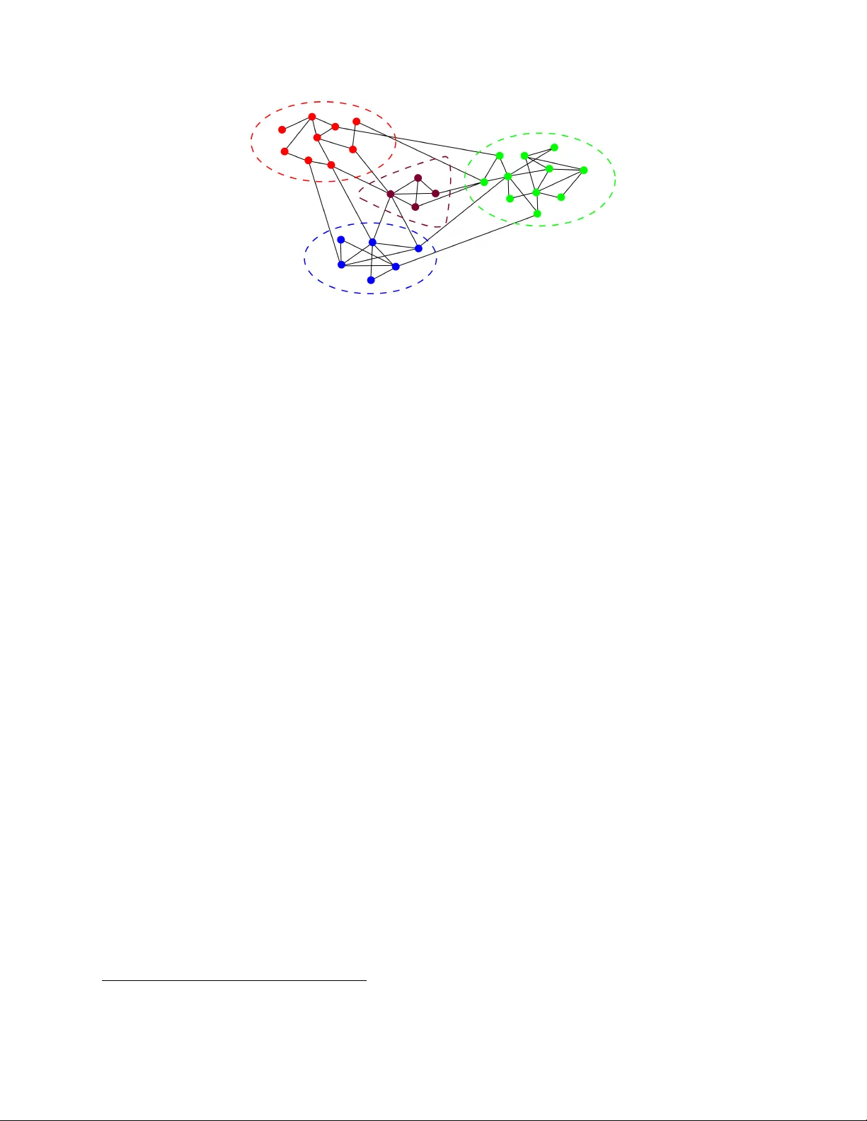
Basic mo dels and questions in statistical net w ork analysis Mikl´ os Z. R´ acz ∗ with S ´ ebastien Bub ec k † Septem b er 13, 2016 Abstract Extracting information from large graphs has b ecome an imp ortan t statistical problem since net work data is now common in v arious ﬁelds. In this minicourse w e will in vestigate the most natural statistical questions for three canonical probabilistic mo dels of net works: (i) comm unity detection in the stochastic blo c k model, (ii) ﬁnding the em b edding of a random geometric graph, and (iii) ﬁnding the original vertex in a preferential attac hment tree. Along the w ay we will co ver many in teresting topics in probabilit y theory suc h as P´ oly a urns, large deviation theory , concen tration of measure in high dimension, entropic central limit theorems, and more. Outline: • Lecture 1: A primer on exact reco very in the general sto c hastic block mo del. • Lecture 2: Estimating the dimension of a random geometric graph on a high-dimensional sphere. • Lecture 3: Introduction to entropic central limit theorems and a pro of of the fundamental limits of dimension estimation in random geometric graphs. • Lectures 4 & 5: Conﬁdence sets for the ro ot in uniform and preferential attachmen t trees. Ac kno wledgements These notes were prepared for a minicourse presen ted at Univ ersity of W ashington during June 6–10, 2016, and at the XX Brazilian School of Probability held at the S˜ ao Carlos campus of Univ ersidade de S˜ ao P aulo during July 4–9, 2016. W e thank the organizers of the Brazilian Sc ho ol of Probabilit y , P aulo F aria da V eiga, Rob erto Im buzeiro Oliv eira, Leandro Pimen tel, and Luiz Renato F on tes, for in viting us to presen t a minicourse on this topic. W e also thank Sham Kak ade, Anna Karlin, and Marina Meila for help with organizing at Univ ersity of W ashington. Man y thanks to all the participan ts who ask ed go o d questions and provided useful feedback, in particular Kira Goldner, Chris Hoﬀman, Jacob Richey , and Ryokic hi T anak a in Seattle, and Vladimir Belitsky , Santiago Duran, Simon Griﬃths, and Rob erto Im buzeiro Oliveira in S˜ ao Carlos. ∗ Microsoft Research; miracz@microsoft.com . † Microsoft Research; sebubeck@microsoft.com . 1 1 Lecture 1: A primer on exact reco v ery in the general sto c hastic blo c k mo del Comm unity detection is a fundamental problem in man y sciences, such as sociology (e.g., ﬁnding tigh t-knit groups in so cial netw orks), biology (e.g., detecting protein complexes), and b ey ond. Giv en its importance, there hav e been a plethora of algorithms developed in the past few decades to detect comm unities. But how can w e test whether an algorithm p erforms w ell? What are the fundamen tal limits to any communit y detection algorithm? Often in real data the ground truth is not known (or there is not even a well-deﬁned ground truth), so judging the performance of algorithms can b e diﬃcult. Probabilistic generative mo dels can b e used to mo del real netw orks, and even if they do not ﬁt the data perfectly , they can still b e useful: they can act as b enc hmarks for comparing diﬀeren t clustering algorithms, since the ground truth is known. P erhaps the most widely studied generative mo del that exhibits communit y structure is the sto c hastic block mo del (SBM). The SBM w as ﬁrst introduced in so ciology [29] and was then studied in several diﬀeren t scien tiﬁc c omm unities, including mathematics, computer science, ph ysics, and statistics [18, 19, 27, 9, 35, 44]. 1 It giv es a distribution on graphs with n vertices with a hidden partition of the nodes in to k comm unities. The relative sizes of the communities, and the edge densities connecting comm unities are parameters of the general SBM. The statistical inference problem is then to recov er as muc h of the communit y structure as p ossible given a realization of the graph, but without knowing any of the comm unit y labels. 1.1 The sto c hastic blo c k mo del and notions of recov ery The general sto c hastic blo c k mo del is a distribution on graphs with latent communit y structure, and it has three parameters: n , the n umber of v ertices; a probabilit y distribution p = ( p 1 , . . . , p k ) that describ es the relative sizes of the communities; and Q ∈ [0 , 1] k × k , a symmetric k × k matrix that describ es the probabilities with which t wo giv en vertices are connected, dep ending on which comm unities they b elong to. The num b er of comm unities, k , is implicit in this notation; in these notes we assume that k is a ﬁxed constant. A random graph from SBM( n, p, Q ) is deﬁned as follo ws: • The vertex set of the graph is V = { 1 , . . . , n } ≡ [ n ]. • Ev ery vertex v ∈ V is indep endently assigned a (hidden) label σ v ∈ [ k ] from the probabilit y distribution p on [ k ]. That is, P ( σ v = i ) = p i for every i ∈ [ k ]. • Giv en the lab els of the v ertices, each (unordered) pair of v ertices ( u, v ) ∈ V × V is connected indep enden tly with probabilit y Q σ u ,σ v . Example 1.1 (Symmetric comm unities) . A simple example to ke ep in mind is that of symmetric c ommunities, with mor e e dges within c ommunities than b etwe en c ommunities. This is mo dele d by the SBM with p i = 1 /k for al l i ∈ [ k ] and Q i,j = a if i = j and Q i,j = b otherwise, with a > b > 0 . W e write G ∼ SBM( n, p, Q ) for a graph generated according to the SBM without the hidden v ertex labels rev ealed. The goal of a statistical inference algorithm is to reco ver as many lab els as p ossible using only the underlying graph as an observ ation. There are v arious notions of success that are w orth studying. 1 Disclaimer: the literature on communit y detection is v ast and rapidly growing. It is not our inten t here to survey this literature; we refer the interested reader to the pap ers we cite for further references. 2 Figure 1: A sc hematic of the general stochastic blo c k mo del. • W eak recov ery (also known as detection). An algorithm is said to we akly r e c over or dete ct the communities if it outputs a partition of the no des whic h is p ositiv ely correlated with the true partition, with high probability (whp) 2 . • P artial reco very . How muc h can b e recov ered ab out the communities? An algorithm is said to r e c over c ommunities with an ac cur acy of α ∈ [0 , 1] if it outputs a lab elling of the no des whic h agrees with the true labelling on a fraction α of the no des whp. An imp ortan t sp ecial case is when only o ( n ) v ertices are allow ed to b e misclassiﬁed whp, known as we ak c onsistency or almost exact r e c overy . • Exact reco very (also known as reco very or strong consistency). The strongest notion of reconstruction is to reco ver the labels of all vertices exactly whp. When this is not possible, it can still b e of interest to understand which communities can b e exactly reco vered, if not all; this is sometimes known as “p artial-exact-r e c overy” . In all the notions abov e, the agreemen t of a partition with the true partition is maximized ov er all relab ellings of the comm unities, since we are not in terested in the speciﬁc original labelling per se, but rather the partition (comm unity structure) it induces. The diﬀerent notions of reco very naturally lead to studying diﬀerent regimes of the parameters. F or weak reco v ery to b e possible, man y v ertices in all but one communit y should b e non-isolated (in the symmetric case this means that there should b e a giant comp onen t), requiring the edge probabilities to b e Ω (1 /n ). F or exact recov ery , all vertices in all but one communit y should b e non-isolated (in the symmetric case this means that the graph should be connected), requiring the edge probabilities to b e Ω (ln( n ) /n ). In these regimes it is natural to scale the edge probability matrices accordingly , i.e., to consider SBM ( n, p, Q/n ) or SBM ( n, p, ln ( n ) Q/n ), where Q ∈ R k × k + . There has b een lots of w ork in the past few years understanding the fundamental limits to reco very under the v arious notions discussed ab ov e. F or w eak reco very there is a sharp phase transition, the threshold of whic h was ﬁrst conjectured in [21]. This w as prov en ﬁrst for tw o symmetric comm unities [39, 40] and then for multiple communities [3]. Partial recov ery is less well understo od, and ﬁnding the fraction of no des that can b e correctly recov ered for a given set of parameters is an op en problem; see [41] for results in this direction for tw o symmetric comm unities. In this lecture w e are in terested in exact reco very , for whic h Abb e and Sandon ga ve the v alue of the threshold for the general SBM, and sho wed that a quasi-linear time algorithm w orks all the w ay 2 In these notes “with high probabilit y” stands for with probabilit y tending to 1 as the num b er of no des in the graph, n , tends to inﬁnity . 3 to the threshold [2] (building on previous work that determined the threshold for tw o symmetric comm unities [1, 42]). The remainder of this lecture is an exposition of their main results and a few of the k ey ideas that go in to proving and understanding it. 1.2 F rom exact reco very to testing m ultiv ariate Poisson distributions Recall that we are interested in the logarithmic degree regime for exact reco very , i.e., we consider G ∼ SBM( n, p, ln( n ) Q/n ), where Q ∈ R k × k + is indep enden t of n . W e also assume that the com- m unities hav e linear size, i.e., that p is indep enden t of n , and p i ∈ (0 , 1) for all i . Our goal is to reco ver the lab els of all the v ertices whp. As a though t exp erimen t, imagine that not only is the graph G giv en, but also all v ertex lab els are revealed, except for that of a giv en v ertex v ∈ V . Is it p ossible to determine the lab el of v ? Figure 2: Supp ose all communit y labels are known except that of v ertex v . Can the lab el of v b e determined based on its neighbors’ lab els? Understanding this question is key for understanding exact reco very , since if the error probability of this is to o high, then exact recov ery will not b e possible. On the other hand, it turns out that in this regime it is p ossible to reco ver all but o ( n ) lab els using an initial partial recov ery algorithm. The setup of the thought exp erimen t then b ecomes relev an t, and if w e can determine the lab el of v given the lab els of all the other no des with low error probabilit y , then w e can correct all errors made in the initial partial reco very algorithm, leading to exact reco very . W e will come back to the connection b et w een the thought experiment and exact reco v ery; for no w we focus on understanding this thought exp erimen t. Giv en the labels of all vertices except v , the information we ha ve ab out v is the num b er of no des in eac h comm unity it is connected to. In other w ords, w e kno w the de gr e e pr oﬁle d ( v ) of v , where, for a given lab elling of the graph’s vertices, the i -th comp onen t d i ( v ) is the num b er of edges b et w een v and the v ertices in comm unity i . The distribution of the degree proﬁle d ( v ) dep ends on the communit y that v b elongs to. Recall that the communit y sizes are giv en b y a multinomial distribution with parameters n and p , and hence the relativ e size of comm unit y i ∈ [ k ] concen trates on p i . Th us if σ v = j , the degree proﬁle d ( v ) = ( d 1 ( v ) , . . . , d k ( v )) can be approximated b y indep enden t binomials, with d i ( v ) appro ximately distributed as Bin ( np i , ln( n ) Q i,j /n ), where Bin( m, q ) denotes the binomial distribution with m trials and success probability q . In this regime, the binomial distribution is w ell-approximated by a Poisson distribution of the same mean. In particular, Le Cam’s inequalit y giv es that TV (Bin ( na, ln( n ) b/n ) , Poi ( ab ln( n ))) ≤ 2 ab 2 (ln( n )) 2 n , 4 where P oi ( λ ) denotes the Poisson distribution with mean λ , and TV denotes the total v ariation distance 3 . Using the additivit y of the Poisson distribution and the triangle inequality , we get that TV   L ( d ( v )) , P oi   ln ( n ) X i ∈ [ k ] p i Q i,j e i     = O (ln ( n )) 2 n ! , where L ( d ( v )) denotes the law of d ( v ) conditionally on σ v = j and e i is the i -th unit vector. Th us the degree proﬁle of a vertex in communit y j is appro ximately P oisson distributed with mean ln ( n ) P i ∈ [ k ] p i Q i,j e i . Deﬁning P = diag( p ), this can b e abbreviated as ln ( n ) ( P Q ) j , where ( P Q ) j denotes the j -th column of the matrix P Q . W e call the quan tity ( P Q ) j the c ommunity pr oﬁle of communit y j ; this is the quantit y that determines the distribution of the degree proﬁle of vertices from a giv en comm unity . Our thought exp erimen t has thus b een reduced to a Bay esian hypothesis testing problem b e- t ween k multiv ariate Poisson distributions. The prior on the lab el of v is given b y p , and we get to observ e the degree proﬁle d ( v ), which comes from one of k m ultiv ariate Poisson distributions, whic h ha v e mean ln( n ) times the communit y proﬁles ( P Q ) j , j ∈ [ k ]. 1.3 T esting m ultiv ariate Poisson distributions W e now turn to understanding the testing problem describ ed ab o ve; the setup is as follo ws. W e consider a Ba y esian hypothesis testing problem with k hypotheses. The random v ariable H tak es v alues in [ k ] with prior giv en by p , i.e., P ( H = j ) = p j . W e do not observe H , but instead we observ e a dra w from a multiv ariate Poisson distribution whose mean dep ends on the realization of H : given H = j , the mean is λ ( j ) ∈ R k + . In short: D | H = j ∼ Poi ( λ ( j )) , j ∈ [ k ] . In more detail: P ( D = d | H = j ) = P λ ( j ) ( d ) , d ∈ Z k + , where P λ ( j ) ( d ) = Y i ∈ [ k ] P λ i ( j ) ( d i ) and P λ i ( j ) ( d i ) = λ i ( j ) d i d i ! e − λ i ( j ) . Our goal is to infer the v alue of H from a realization of D . The error probability is minimized by the maximum a p osteriori (MAP) rule, which, up on observing D = d , selects arg max j ∈ [ k ] P ( D = d | H = j ) p j as an estimate for the v alue of H , with ties brok en arbitrarily . Let P e denote the error of the MAP estimator. One can think of the MAP estimator as a tournamen t of k − 1 pairwise comparisons of the hypotheses: if P ( D = d | H = i ) p i > P ( D = d | H = j ) p j then the MAP estimate is not j . The probabilit y that one makes an error during such a comparison is exactly P e ( i, j ) := X x ∈ Z k + min { P ( D = x | H = i ) p i , P ( D = x | H = j ) p j } . (1.1) 3 Recall that the total v ariation distance b et ween tw o random v ariables X and Y taking v alues in a ﬁnite space X with laws µ and ν is deﬁned as TV ( µ, ν ) ≡ TV ( X, Y ) = 1 2 P x ∈X | µ ( x ) − ν ( x ) | = sup A | µ ( A ) − ν ( A ) | . 5 F or ﬁnite k , the error of the MAP estimator is on the same order as the largest pairwise comparison error, i.e., max i,j P e ( i, j ). In particular, we ha ve that 1 k − 1 X i 0 , we have X x ∈ Z k + min  P ln( n ) c 1 ( x ) p 1 , P ln( n ) c 2 ( x ) p 2  = O n − D + ( c 1 ,c 2 ) − ln ln( n ) 2 ln( n ) ! , (1.3) X x ∈ Z k + min  P ln( n ) c 1 ( x ) p 1 , P ln( n ) c 2 ( x ) p 2  = Ω n − D + ( c 1 ,c 2 ) − k ln ln( n ) 2 ln( n ) ! , (1.4) wher e D + ( c 1 , c 2 ) = max t ∈ [0 , 1] X i ∈ [ k ]  tc 1 ( i ) + (1 − t ) c 2 ( i ) − c 1 ( i ) t c 2 ( i ) 1 − t  . (1.5) W e do not go o ver the pro of of this statemen t—which w e leav e to the reader as a c hallenging exercise—but we provide some intuition in the univ ariate case. Figure 3 illustrates the probabilit y mass function of t wo P oisson distributions, with means λ = 20 and µ = 30, respectively . Observe that min {P λ ( x ) , P µ ( x ) } decays rapidly a wa y from x max := arg max x ∈ Z + min {P λ ( x ) , P µ ( x ) } , so Figure 3: T esting univ ariate P oisson distributions. The ﬁgure plots the probabilit y mass function of tw o Poisson distributions, with means λ = 20 and µ = 30, resp ectiv ely . 6 w e can obtain a go o d estimate of the sum P x ∈ Z + min {P λ ( x ) , P µ ( x ) } by simply estimating the term min {P λ ( x max ) , P µ ( x max ) } . Now observ e that x max m ust satisfy P λ ( x max ) ≈ P µ ( x max ); after some algebra this is equiv alent to x max ≈ λ − µ log( λ/µ ) . Let t ∗ denote the maximizer in the expression of D + ( λ, µ ) in (1.5). By diﬀeren tiating in t , w e obtain that t ∗ satisﬁes λ − µ − log ( λ/µ ) · λ t ∗ µ 1 − t ∗ = 0, and so λ t ∗ µ 1 − t ∗ = λ − µ log( λ/µ ) . Th us w e see that x max ≈ λ t ∗ µ 1 − t ∗ , from which, after some algebra, we get that P λ ( x max ) ≈ P µ ( x max ) ≈ exp ( − D + ( λ, µ )). The pro of of (1.4) in the m ultiv ariate case follows along the same lines: the s ingle term cor- resp onding to x max := arg max x ∈ Z k + min  P ln( n ) c 1 ( x ) , P ln( n ) c 2 ( x )  giv es the low er b ound. F or the upp er b ound of (1.3) one has to sho w that the other terms do not con tribute muc h more. Exercise 1.2. Pr ove L emma 1.2. Our conclusion is thus that the error exp onen t in testing multiv ariate Poisson distributions is giv en b y the explicit quan tity D + in (1.5). The discussion in Section 1.2 then implies that D + pla ys an important role in the threshold for exact recov ery . In particular, it intuitiv ely follo ws from Lemma 1.2 that a necess ary condition for exact reco very should be that min i,j ∈ [ k ] ,i 6 = j D +  ( P Q ) i , ( P Q ) j  ≥ 1 . Supp ose on the con trary that D +  ( P Q ) i , ( P Q ) j  < 1 for some i and j . This implies that the error probabilit y in the testing problem is Ω  n ε − 1  for some ε > 0 for all v ertices in comm unities i and j . Since the n umber of v ertices in these comm unities is linear in n , and most of the h yp othesis testing problems are approximately indep endent, one exp ects there to b e no error in the testing problems with probabilit y at most  1 − Ω  n ε − 1  Ω( n ) = exp ( − Ω ( n ε )) = o (1). 1.4 Chernoﬀ-Hellinger div ergence Before mo ving on to the threshold for exact recov ery in the general SBM, w e discuss connections of D + to other, w ell-known measures of div ergence. W riting D t ( µ, ν ) := X x ∈ [ k ]  tµ ( x ) + (1 − t ) ν ( x ) − µ ( x ) t ν ( x ) 1 − t  w e ha v e that D + ( µ, ν ) = max t ∈ [0 , 1] D t ( µ, ν ) . F or any ﬁxed t , D t can b e written as D t ( µ, ν ) = X x ∈ [ k ] ν ( x ) f t  µ ( x ) ν ( x )  , where f t ( x ) = 1 − t + tx − x t , which is a conv ex function. Thus D t is an f -diver genc e , part of a family of div ergences that generalize the Kullbac k-Leibler (KL) div ergence (also known as relativ e entrop y), which is obtained for f ( x ) = x ln( x ). The family of f -divergences with conv ex f share man y useful properties, and hence hav e b een widely studied in information theory and statistics. The sp ecial case of D 1 / 2 ( µ, ν ) = 1 2   √ µ − √ ν   2 2 is kno wn as the Hellinger divergence. The Chernoﬀ div ergence is deﬁned as C ∗ ( µ, ν ) = max t ∈ (0 , 1) − log P x µ ( x ) t ν ( x ) 1 − t , and so if µ and ν are probability vectors, then D + ( µ, ν ) = 1 − e − C ∗ ( µ,ν ) . Because of these connections, Abbe and Sandon termed D + the Chernoﬀ-Hel linger diver genc e . While the quantit y D + still might seem m ysterious, even in ligh t of these connections, a useful p oin t of view is that Lemma 1.2 giv es D + an op er ational me aning . 7 1.5 Characterizing exact reco v erability using CH-div ergence Going bac k to the exact reco very problem in the general SBM, let us jump righ t in and state the reco verabilit y threshold of Abbe and Sandon: exact reco very in SBM( n, p, ln( n ) Q/n ) is possible if and only if the CH-divergence b et ween all pairs of communit y proﬁles is at least 1. Theorem 1.3 (Abb e and Sandon [2]) . L et k ∈ Z + denote the numb er of c ommunities, let p ∈ (0 , 1) k with k p k 1 = 1 denote the c ommunity prior, let P = diag ( p ) , and let Q ∈ (0 , ∞ ) k × k b e a symmetric k × k matrix with no two r ows e qual. Exact r e c overy is solvable in SBM ( n, p, ln( n ) Q/n ) if and only if min i,j ∈ [ k ] ,i 6 = j D +  ( P Q ) i , ( P Q ) j  ≥ 1 . (1.6) This theorem th us provides an op erational meaning to the CH-divergence for the communit y reco very problem. Example 1.4 (Symmetric comm unities) . Consider again k symmetric c ommunities, that is, p i = 1 /k for al l i ∈ [ k ] , Q i,j = a if i = j , and Q i,j = b otherwise, with a, b > 0 . Then exact r e c overy is solvable in SBM ( n, p, ln( n ) Q/n ) if and only if    √ a − √ b    ≥ √ k . (1.7) We note that in this c ase D + is the same as the Hel linger diver genc e. Exercise 1.3. De duc e fr om The or em 1.3 that (1.7) gives the thr eshold in the example ab ove. 1.5.1 Ac hiev ability Let us now see ho w Theorem 1.3 follo ws from the h yp othesis testing results, starting with the ac hiev abilit y . When the condition (1.6) holds, then Lemma 1.2 tells us that in the hypothesis testing problem b et ween P oisson distributions the error of the MAP estimate is o (1 /n ). Thus if the setting of the though t exp erimen t describ ed in Section 1.2 applies to ev ery vertex, then b y lo oking at the degree proﬁles of the v ertices w e can correctly reclassify all v ertices, and the probability that w e make an error is o (1) by a union b ound. How ever, the setting of the thought experiment do es not quite apply . Nonetheless, in this logarithmic degree regime it is p ossible to partially reconstruct the lab els of the v ertices, with only o ( n ) vertices being misclassiﬁed. The details of this partial reconstruction pro cedure w ould require a separate lecture—in brief, it determines whether t wo vertices are in the same communit y or not b y lo oking at how their log( n ) size neigh b orho o ds in teract—so no w we will tak e this for gran ted. It is p ossible to show that there exists a constan t δ suc h that if one estimates the label of a v ertex v based on classiﬁcations of its neighbors that are wrong with probabilit y x , then the probabilit y of misclassifying v is at most n δ x times the probabilit y of error if all the neighbors of v w ere classiﬁed correctly . The issue is that the standard partial recov ery algorithm has a constant error rate for the classiﬁcations, thus the error rate of the degree proﬁling step could b e n c times as large as the error in the h yp othesis testing problem, for some c > 0. This is an issue when min i 6 = j D +  ( P Q ) i , ( P Q ) j  < 1 + c . T o get around this, one can do multiple rounds of more accurate classiﬁcations. First, one obtains a partial reconstruction of the lab els with an error rate that is a suﬃcien tly lo w constan t. After applying the degree-proﬁling step to eac h vertex, the classiﬁcation error at each v ertex is now O ( n − c 0 ) for some c 0 > 0. Hence after applying another degree-proﬁling step to each vertex, the classiﬁcation error at eac h v ertex will no w be at most n δ × O ( n − c 0 ) × o (1 /n ) = o (1 /n ). Th us applying a union bound at this stage w e can conclude that all vertices are correctly labelled whp. 8 1.5.2 Imp ossibilit y The necessit y of condition (1.6) w as already describ ed at a high level at the end of Section 1.3. Here we giv e some details on ho w to deal with the dep endencies that arise. Assume that (1.6) do es not hold, and let i and j be tw o communities that violate the condition, i.e., for which D +  ( P Q ) i , ( P Q ) j  < 1. W e w ant to argue that vertices in comm unities i and j cannot all b e distinguished, and so any classiﬁcation algorithm has to make at least one error whp. An important fact that w e use is that the low er b ound (1.4) arises from a particular c hoice of degree proﬁle that is b oth likely for the t w o comm unities. Namely , deﬁne the degree proﬁle x b y x ` = j ( P Q ) t ∗ `,i ( P Q ) 1 − t ∗ `,j ln ( n ) k for every ` ∈ [ k ], where t ∗ ∈ [0 , 1] is the maximizer in D +  ( P Q ) i , ( P Q ) j  , i.e., the v alue for whic h D +  ( P Q ) i , ( P Q ) j  = D t ∗  ( P Q ) i , ( P Q ) j  . Then Lemma 1.2 tells us that for any vertex in communit y i or j , the probabilit y that it has degree proﬁle x is at least Ω  n − D + ( ( P Q ) i , ( P Q ) j ) / (ln ( n )) k/ 2  , whic h is at least Ω  n ε − 1  for some ε > 0 b y assumption. T o sho w that this holds for man y vertices in comm unities i and j at once, we ﬁrst select a random set S of n/ (ln ( n )) 3 v ertices. Whp the in tersection of S with any communit y ` is within √ n of the exp ected v alue p ` n/ (ln ( n )) 3 , and furthermore a randomly selected v ertex in S is not connected to any other v ertex in S . Thus the distribution of a v ertex’s degree proﬁle excluding connections to vertices in S is essen tially a m ultiv ariate P oisson distribution as before. W e call a vertex in S ambiguous if for each ` ∈ [ k ] it has exactly x ` neigh b ors in communit y ` that are not in S . By Lemma 1.2 w e ha ve that a v ertex in S that is in communit y i or j is ambiguous with probability Ω  n ε − 1  . By deﬁnition, for a ﬁxed comm unity assignmen t and choice of S , there is no dep endence on whether t wo vertices are am biguous. F urthermore, due to the c hoice of the size of S , whp there are at least ln ( n ) ambiguous v ertices in comm unity i and at least ln ( n ) am biguous vertices in communit y j that are not adjacen t to an y other v ertices in S . These 2 ln ( n ) are indistinguishable, so no algorithm classiﬁes all of them correctly with probabilit y greater than 1 /  2 ln( n ) ln( n )  , which tends to 0 as n → ∞ . 1.5.3 The ﬁnest exact partition recov erable W e conclude b y men tioning that this threshold generalizes to ﬁner questions. If exact reco very is not p ossible, what is the ﬁnest partition that can b e reco vered? W e say that exact reco very is solv able for a communit y partition [ k ] = t t s =1 A s , where A s is a subset of [ k ], if there exists an algorithm that whp assigns to ev ery v ertex an elemen t of { A 1 , . . . , A t } that con tains its true communit y . The ﬁnest partition that is exactly recov erable can also be expressed using CH-divergence in a similar fashion. It is the largest collection of disjoin t subsets suc h that the CH-divergence betw een these subsets is at least 1, where the CH-divergence b et w een t wo subsets is deﬁned as the minimum of the CH-divergences b et ween an y t wo communit y proﬁles in these subsets. Theorem 1.5 (Abb e and Sandon [2]) . Under the same settings as in The or em 1.3, exact r e c overy is solvable in SBM ( n, p, ln( n ) Q/n ) for a p artition [ k ] = t t s =1 A s if and only if D +  ( P Q ) i , ( P Q ) j  ≥ 1 for every i and j in diﬀer ent subsets of the p artition. 9 2 Lecture 2: Estimating the dimension of a random geometric graph on a high-dimensional sphere Man y real-world net works ha ve strong structural features and our goal is often to reco ver these hid- den structures. In the previous lecture w e studied the fundamen tal limits of inferring communities in the sto c hastic blo c k mo del, a natural generative mo del for graphs with communit y structure. Another p ossibilit y is ge ometric structur e . Man y netw orks coming from physical considerations naturally hav e an underlying geometry , such as the netw ork of ma jor roads in a coun try . In other net works this stems from a latent feature space of the no des. F or instance, in so cial net works a p erson migh t b e represented b y a feature v ector of their in terests, and t wo p eople are connected if their interests are close enough; this laten t metric space is referred to as the so cial sp ac e [28]. In suc h net works the natural questions prob e the underlying geometry . Can one detect the presence of geometry? If so, can one estimate v arious aspects of the geometry , e.g., an appropriately deﬁned dimension? In this lecture we study these questions in a particularly natural and simple generativ e mo del of a random geometric graph: n p oin ts are pic ked uniformly at random on the d -dimensional sphere, and tw o p oin ts are connected by an edge if and only if they are suﬃcently close. 4 W e are particularly interested in the high-dimensional regime, motiv ated b y recent adv ances in all areas of applied mathematics, and in particular statistics and learning theory , where high- dimensional feature spaces are b ecoming the new norm. While the low-dimensional regime has b een studied for a long time in probability theory [43], the high-dimensional regime brings ab out a host of new and interesting questions. 2.1 A simple random geometric graph mo del and basic questions Let us no w deﬁne more precisely the random geometric graph model w e consider and the questions w e study . In general, a geometric graph is such that eac h vertex is lab eled with a p oin t in some metric space, and an edge is presen t b et ween t w o vertices if the distance betw een the corresp onding lab els is smaller than some presp eciﬁed threshold. W e focus on the case where the underlying metric space is the Euclidean sphere S d − 1 =  x ∈ R d : k x k 2 = 1  , and the laten t lab els are i.i.d. uniform random v ectors in S d − 1 . W e denote this mo del by G ( n, p, d ), where n is the num b er of v ertices and p is the probability of an edge b et ween t wo v ertices ( p determines the threshold distance for connection). This model is closely related to laten t space approac hes to social net work analysis [28]. Sligh tly more formally , G ( n, p, d ) is deﬁned as follows. Let X 1 , . . . , X n b e indep enden t random v ectors, uniformly distributed on S d − 1 . In G ( n, p, d ), distinct v ertices i ∈ [ n ] and j ∈ [ n ] are connected by an edge if and only if h X i , X j i ≥ t p,d , where the threshold v alue t p,d ∈ [ − 1 , 1] is suc h that P ( h X 1 , X 2 i ≥ t p,d ) = p . F or example, when p = 1 / 2 w e hav e t p,d = 0. The most natural random graph model without an y structure is the standard Erd˝ os-R ´ en yi ran- dom graph G ( n, p ), where any t wo of the n vertices are indep enden tly connected with probabilit y p . W e can th us formalize the question of detecting underlying geometry as a simple hypothesis testing question. The null h yp othesis is that the graph is dra wn from the Erd˝ os-R ´ en yi mo del, while the alternative is that it is dra wn from G ( n, p, d ). In brief: H 0 : G ∼ G ( n, p ) , H 1 : G ∼ G ( n, p, d ) . (2.1) T o understand this question, the basic quantit y we need to study is the total v ariation distance b et w een the tw o distributions on graphs, G ( n, p ) and G ( n, p, d ), denoted by TV ( G ( n, p ) , G ( n, p, d )); 4 This lecture is based on [14]. 10 recall that the total v ariation distance b et ween tw o probabilit y measures P and Q is deﬁned as TV ( P , Q ) = 1 2 k P − Q k 1 = sup A | P ( A ) − Q ( A ) | . W e are interested in particular in the case when the dimension d is lar ge , gro wing with n . It is in tuitively clear that if the geometry is too high-dimensional, then it is imp ossible to detect it, while a low-dimensional geometry will hav e a strong eﬀect on the generated graph and will b e detectable. How fast can the dimension grow with n while still b eing able to detect it? Most of this lecture will fo cus on this question. If w e can detect geometry , then it is natural to ask for more information. Perhaps the ultimate goal would b e to ﬁnd an embedding of the vertices into an appropriate dimensional sphere that is a true r epr esentation , in the sense that the geometric graph formed from the embedded p oin ts is indeed the original graph. More mo destly , can the dimension b e estimated? W e touch on this question at the end of the lecture. 2.2 The dimension threshold for detecting underlying geometry The high-dimensional setting of the random geometric graph G ( n, p, d ) w as ﬁrst studied by Devro ye, Gy¨ orgy , Lugosi, and Udina [22], who show ed that if n is ﬁxed and d → ∞ , then TV ( G ( n, p ) , G ( n, p, d )) → 0 , that is, geometry is indeed lost in high dimensions. More precisely , they show that this conv er- gence happ ens when d  n 7 2 n 2 / 2 . 5 This follo ws by observing that for ﬁxed n , the multiv ariate cen tral limit theorem implies that as d → ∞ , the inner pro ducts of the latent vectors con verge in distribution to a standard Gaussian:  1 √ d h X i , X j i  { i,j }∈ ( [ n ] 2 ) d →∞ = ⇒ N  0 , I ( n 2 )  . The Berry-Esseen theorem gives a con vergence rate, whic h then allo ws to show that for an y graph G on n vertices, | P ( G ( n, p ) = G ) − P ( G ( n, p, d ) = G ) | = O  p n 7 /d  ; the factor of 2 n 2 / 2 comes from applying this b ound to ev ery term in the L 1 distance. Ho wev er, the result ab o ve is not tigh t, and we seek to understand the fundamen tal limits to detecting underlying geometry . The dimension threshold for dense graphs was recen tly found in [14], and it turns out that it is d ≈ n 3 , in the following sense. Theorem 2.1 (Bub eck, Ding, Eldan, R´ acz [14]) . L et p ∈ (0 , 1) b e ﬁxe d. Then TV ( G ( n, p ) , G ( n, p, d )) →  0 , if d  n 3 , (2.2) 1 , if d  n 3 . (2.3) Mor e over, in the latter c ase ther e exists a c omputational ly eﬃcient test to dete ct underlying ge om- etry (with running time O  n 3  ). Most of the lecture will b e devoted to understanding this theorem. A t the end w e will consider this same question for sp arse gr aphs (where p = c/n ), where determining the dimension threshold is an in triguing op en problem. 5 Throughout these notes we use standard asymptotic notation; for instance, f ( t )  g ( t ) as t → ∞ if lim t →∞ f ( t ) /g ( t ) = 0. 11 2.3 The triangle test A natural test to unco v er geometric structure is to count the num b er of triangles in G . Indeed, in a purely random scenario, vertex u being connected to b oth v and w says nothing about whether v and w are connected. On the other hand, in a geometric setting this implies that v and w are close to each other due to the triangle inequality , thus increasing the probabilit y of a connection betw een them. This, in turn, implies that the expected n umber of triangles is larger in the geometric setting, giv en the same edge densit y . Let us now compute what this statistic gives us. Figure 4: Giv en that u is connected to b oth v and w , v and w are more likely to b e connected under G ( n, p, d ) than under G ( n, p ). F or a graph G , let A denote its adjacency matrix, i.e., A i,j = 1 if v ertices i and j are connected, and 0 otherwise. Then T G ( i, j, k ) := A i,j A i,k A j,k is the indicator v ariable that three v ertices i , j , and k form a triangle, and so the n umber of triangles in G is T ( G ) := X { i,j,k }∈ ( [ n ] 3 ) T G ( i, j, k ) . By linearity of expectation, for b oth mo dels the exp ected n umber of triangles is  n 3  times the probabilit y of a triangle b et w een three sp eciﬁc vertices. F or the Erd˝ os-R´ enyi random graph the edges are independent, so the probabilit y of a triangle is p 3 , and th us we hav e E [ T ( G ( n, p ))] =  n 3  p 3 . F or G ( n, p, d ) it turns out that for an y ﬁxed p ∈ (0 , 1) we ha ve P  T G ( n,p,d ) (1 , 2 , 3) = 1  ≈ p 3  1 + C p √ d  (2.4) for some constan t C p > 0, which giv es that E [ T ( G ( n, p, d ))] ≥  n 3  p 3  1 + C p √ d  . Sho wing (2.4) is somewhat inv olved, but in essence it follo ws from the c onc entr ation of me asur e phenomenon on the sphere, namely that most of the mass on the high-dimensional sphere is lo cated in a band of O  1 / √ d  around the equator. W e sk etch here the main in tuition for p = 1 / 2, whic h is illustrated in Figure 5. Let X 1 , X 2 , and X 3 b e indep enden t uniformly distributed p oin ts in S d − 1 . Then P  T G ( n, 1 / 2 ,d ) (1 , 2 , 3) = 1  = P ( h X 1 , X 2 i ≥ 0 , h X 1 , X 3 i ≥ 0 , h X 2 , X 3 i ≥ 0) = P ( h X 2 , X 3 i ≥ 0 | h X 1 , X 2 i ≥ 0 , h X 1 , X 3 i ≥ 0) P ( h X 1 , X 2 i ≥ 0 , h X 1 , X 3 i ≥ 0) = 1 4 × P ( h X 2 , X 3 i ≥ 0 | h X 1 , X 2 i ≥ 0 , h X 1 , X 3 i ≥ 0) , 12 where the last equality follows b y indep endence. So what remains is to show that this latter conditional probability is appro ximately 1 / 2 + c/ √ d . T o compute this conditional probability what w e really need to kno w is the typical angle is betw een X 1 and X 2 . By rotational inv ariance w e may assume that X 1 = (1 , 0 , 0 , . . . , 0), and hence h X 1 , X 2 i = X 2 (1), the ﬁrst co ordinate of X 2 . One w ay to generate X 2 is to sample a d -dimensional standard Gaussian and then normalize it by its length. Since the norm of a d -dimensional standard Gaussian is v ery w ell concen trated around √ d , it follo ws that X 2 (1) is on the order of 1 / √ d . Conditioned on X 2 (1) ≥ 0, this typical angle giv es the b o ost in the conditional probability that we see. See Figure 5 for an illustration. Figure 5: If X 1 and X 2 are tw o independent uniform p oin ts on the d -dimensional sphere S d − 1 , then their inner pro duct h X 1 , X 2 i is on the order of 1 / √ d due to the concen tration of measure phenomenon on the sphere. This then implies that the probabilit y of a triangle in G ( n, 1 / 2 , d ) is (1 / 2) 3 + c/ √ d for some constant c > 0. Th us w e see that the b o ost in the n umber of triangles in the geometric setting is Θ  n 3 / √ d  in exp ectation: E [ T ( G ( n, p, d ))] − E [ T ( G ( n, p ))] ≥  n 3  C p √ d . T o b e able to tell apart the t wo graph distributions based on the n umber of triangles, the bo ost in exp ectation needs to be m uch greater than the standard deviation. Exercise 2.1. Show that V ar ( T ( G ( n, p ))) =  n 3   p 3 − p 6  +  n 4  4 2   p 5 − p 6  and that V ar ( T ( G ( n, p, d ))) ≤ n 4 . 13 Exercise 2.2. Show that if | E [ T ( G ( n, p, d ))] − E [ T ( G ( n, p ))] |  max n p V ar ( T ( G ( n, p ))) , p V ar ( T ( G ( n, p, d ))) o , then TV ( G ( n, p ) , G ( n, p, d )) → 1 . Putting together Exercises 2.1 and 2.2 we see that TV ( G ( n, p ) , G ( n, p, d )) → 1 if n 3 / √ d  √ n 4 , whic h is equiv alent to d  n 2 . 2.4 Signed triangles are more p o w erful While triangles detect geometry up un til d  n 2 , are there ev en more pow erful statistics that detect geometry for larger dimensions? One can c heck that longer cycles also only w ork when d  n 2 , as do sev eral other natural statistics. Y et it turns out that the underlying geometry can be detected ev en when d  n 3 . The simple idea that leads to this improv ement is to consider signe d triangles . W e hav e already noticed that triangles are more likely in the geometric setting than in the purely random setting. This also means that induced wedges (i.e., when there are exactly tw o edges among the three p ossible ones) are less likely in the geometric setting. Similarly , induced single edges are more lik ely , and induced indep enden t sets on three v ertices are less likely in the geometric setting. Figure 6 summarizes these observ ations. Figure 6: This ﬁgure summarizes which patterns are more or less likely in the geometric setting than in the purely random setting. The signed triangles statistic rew eights the diﬀerent patterns with p ositiv e and negative w eights. The signed triangles statistic incorp orates these observ ations by giving the diﬀeren t patterns p ositiv e or negativ e weigh ts. More precisely , we deﬁne τ ( G ) := X { i,j,k }∈ ( [ n ] 3 ) ( A i,j − p ) ( A i,k − p ) ( A j,k − p ) . The k ey insight motiv ating this deﬁnition is that the v ariance of signed triangles is much smal ler than the v ariance of triangles, due to the cancellations introduced by the centering of the adjacency matrix: the Θ  n 4  term v anishes, leaving only the Θ  n 3  term. Exercise 2.3. Show that E [ τ ( G ( n, p ))] = 0 and V ar ( τ ( G ( n, p ))) =  n 3  p 3 (1 − p ) 3 . 14 On the other hand it can b e shown that E [ τ ( G ( n, p, d ))] ≥ c p n 3 / √ d, (2.5) so the gap b et w een the exp ectations remains. F urthermore, it can also b e sho wn that the v ariance also decreases for G ( n, p, d ) and w e ha v e V ar ( τ ( G ( n, p, d ))) ≤ n 3 + 3 n 4 d . (2.6) Putting ev erything together and using Exercise 2.2 for the signed triangles statistic τ , w e get that TV ( G ( n, p ) , G ( n, p, d )) → 1 if n 3 / √ d  p n 3 + n 4 /d , whic h is equiv alen t to d  n 3 . This concludes the proof of (2.3) from Theorem 2.1. 2.5 Barrier to detecting geometry: when Wishart b ecomes GOE W e no w turn to proving (2.2), whic h, together with (2.3), shows that the threshold dimension for detecting geometry is n 3 . This also s ho ws that the signed triangle statistic is near-optimal, since it can detect geometry whenever d  n 3 . There are essentially three main wa ys to b ound the total v ariation of t wo distributions from ab o v e: (i) if the distributions ha ve nice form ulas asso ciated with them, then exact computation is p ossible; (ii) through c oupling the distributions; or (iii) by using inequalities b et ween probabilit y metrics to switc h the problem to b ounding a diﬀerent notion of distance betw een the distributions. Here, while the distribution of G ( n, p, d ) do es not hav e a nice formula associated with it, the main idea is to view this random geometric graph as a function of an n × n Wishart matrix with d degrees of freedom—i.e., a matrix of inner products of n d -dimensional Gaussian vectors—denoted b y W ( n, d ). It turns out that one can view G ( n, p ) as (essentially) the same function of an n × n GOE random matrix—i.e., a symmetric matrix with i.i.d. Gaussian en tries on and abov e the diagonal— denoted by M ( n ). The upside of this is that b oth of these random matrix ensem bles ha v e explicit densities that allow for explicit computation. W e explain this connection here in the sp ecial case of p = 1 / 2 for simplicit y; see [14] for the case of general p . Recall that if Y 1 is a standard normal random v ariable in R d , then Y 1 / k Y 1 k is uniformly dis- tributed on the sphere S d − 1 . Consequently w e can view G ( n, 1 / 2 , d ) as a function of an appropriate Wishart matrix, as follows. Let Y b e an n × d matrix where the en tries are i.i.d. standard normal random v ariables, and let W ≡ W ( n, d ) = Y Y T b e the corresp onding n × n Wishart matrix. Note that W ii = h Y i , Y i i = k Y i k 2 and so h Y i / k Y i k , Y j / k Y j ki = W ij / p W ii W j j . Th us the n × n matrix A deﬁned as A i,j = ( 1 if W ij ≥ 0 and i 6 = j 0 otherwise has the same law as the adjacency matrix of G ( n, 1 / 2 , d ). Denote the map that takes W to A b y H , i.e., A = H ( W ). In a similar w ay we can view G ( n, 1 / 2) as a function of an n × n matrix dra wn from the Gaussian Orthogonal Ensem ble (GOE). Let M ( n ) b e a symmetric n × n random matrix where the diagonal en tries are i.i.d. normal random v ariables with mean zero and v ariance 2, and the entries ab o ve the diagonal are i.i.d. standard normal random v ariables, with the en tries on and ab ov e the diagonal all independent. Then B = H ( M ( n )) has the same la w as the adjacency matrix of G ( n, p ). Note that B only dep ends on the sign of the oﬀ-diagonal elemen ts of M ( n ), so in the deﬁnition of B w e can replace M ( n ) with M ( n, d ) := √ dM ( n ) + dI n , where I n is the n × n iden tity matrix. 15 W e can th us conclude that TV ( G ( n, 1 / 2 , d ) , G ( n, 1 / 2)) = TV ( H ( W ( n, d )) , H ( M ( n, d ))) ≤ TV ( W ( n, d ) , M ( n, d )) . The densities of these t wo random matrix ensem bles are well known. Let P ⊂ R n 2 denote the cone of p ositiv e semideﬁnite matrices. When d ≥ n , W ( n, d ) has the follo wing densit y with resp ect to the Leb esgue measure on P : f n,d ( A ) := (det ( A )) 1 2 ( d − n − 1) exp  − 1 2 T r ( A )  2 1 2 dn π 1 4 n ( n − 1) Q n i =1 Γ  1 2 ( d + 1 − i )  , where T r ( A ) denotes the trace of the matrix A . It is also known that the densit y of a GOE random matrix with resp ect to the Leb esgue measure on R n 2 is A 7→ (2 π ) − 1 4 n ( n +1) 2 − n 2 exp  − 1 4 T r  A 2  and so the density of M ( n, d ) with resp ect to the Lebesgue measure on R n 2 is g n,d ( A ) := exp  − 1 4 d T r  ( A − dI n ) 2  (2 π d ) 1 4 n ( n +1) 2 n 2 . These explicit formulas allow for explicit calculations. In particular, one can show that the log-ratio of the densities is o (1) with probabilit y 1 − o (1) according to the measure induced b y M ( n, d ). This follows from writing out the T aylor expansion of the log-ratio of the densities and using kno wn results about the empirical sp ectral distribution of Wigner matrices (in particular that it con verges to a semi-circle law). The outcome of the calculation is the following result, prov en indep enden tly and sim ultaneously by Bub ec k et al. and Jiang and Li. Theorem 2.2 (Bub ec k, Ding, Eldan, R´ acz [14]; Jiang, Li [31]) . Deﬁne the r andom matrix ensem- bles W ( n, d ) and M ( n, d ) as ab ove. If d/n 3 → ∞ , then TV ( W ( n, d ) , M ( n, d )) → 0 . W e conclude that it is imp ossible to detect underlying geometry whenev er d  n 3 . 2.6 Estimating the dimension Un til no w we discussed dete cting geometry . How ev er, the insights gained ab o ve allo w us to also touc h upon the more subtle problem of estimating the underlying dimension d . Dimension estimation can also b e done by counting the “num b er” of signed triangles as in Section 2.4. How ev er, here it is necessary to ha ve a bound on the diﬀerence of the exp ected num b er of signed triangles b et ween consecutiv e dimensions; the low er b ound of (2.5) is not enough. Still, w e believe that the right hand side of (2.5) should giv e the true v alue of the expected v alue for an appropriate constant c p , and hence we expect to hav e that E [ τ ( G ( n, p, d ))] − E [ τ ( G ( n, p, d + 1))] = Θ  n 3 d 3 / 2  . (2.7) Th us, using the v ariance b ound in (2.6), w e get that dimension estimation should b e p ossible using signed triangles whenev er n 3 /d 3 / 2  p n 3 + n 4 /d , which is equiv alent to d  n . Sho wing (2.7) for general p seems inv olved; Bub ec k et al. show ed that it holds for p = 1 / 2, whic h can b e considered as a pro of of concept. W e thus ha ve the following. 16 Theorem 2.3 (Bub ec k, Ding, Eldan, R´ acz [14]) . Ther e exists a universal c onstant C > 0 such that for al l inte gers n and d 1 < d 2 , one has TV ( G ( n, 1 / 2 , d 1 ) , G ( n, 1 / 2 , d 2 )) ≥ 1 − C  d 1 n  2 . This result is tight, as demonstrated by a result of Eldan [24], which states that when d  n , the Wishart matrices W ( n, d ) and W ( n, d + 1) are indistinguishable. By the discussion in Section 2.5, this directly implies that G ( n, 1 / 2 , d ) and G ( n, 1 / 2 , d + 1) are indistinguishable. Theorem 2.4 (Eldan [24]) . Ther e exists a universal c onstant C > 0 such that for al l inte gers n < d , TV ( G ( n, 1 / 2 , d ) , G ( n, 1 / 2 , d + 1)) ≤ TV ( W ( n, d ) , W ( n, d + 1)) ≤ C s  d + 1 d − n  2 − 1 . 2.7 The m ysterious sparse regime The discussion so far has fo cused on dense graphs, i.e., assuming p ∈ (0 , 1) is constan t, where The- orem 2.1 tigh tly characterizes when the underlying geometry can b e detected. The same questions are interesting for sp arse gr aphs as w ell, where the av erage degree is constan t or slowly growing with n . How ev er, since there are so few edges, this regime is muc h more c hallenging. It is again natural to consider the n umber of triangles as a w ay to distin guish b et ween G ( n, c/n ) and G ( n, c/n, d ). A calculation shows that this statistic w orks whenev er d  log 3 ( n ). Theorem 2.5 (Bub ec k, Ding, Eldan, R´ acz [14]) . L et c > 0 b e ﬁxe d and assume d/ log 3 ( n ) → 0 . Then TV  G  n, c n  , G  n, c n , d  → 1 . In contrast with the dense regime, in the sparse regime the signed triangle statistic τ does not giv e signiﬁcantly more p o wer than the triangle statistic T . This is b ecause in the sparse regime, with high probability , the graph do es not contain any 4-vertex subgraph with at least 5 edges, whic h is where the impro vemen t comes from in the dense regime. The authors also conjecture that log 3 ( n ) is the correct order where the transition happ ens. Conjecture 2.6 (Bub ec k, Ding, Eldan, R´ acz [14]) . L et c > 0 b e ﬁxe d and assume d/ log 3 ( n ) → ∞ . Then TV  G  n, c n  , G  n, c n , d  → 0 . The main reason for this conjecture is that, when d  log 3 ( n ), G ( n, c/n ) and G ( n, c/n, d ) seem to be lo cally equiv alent; in particular, they both hav e the same P oisson n umber of triangles asymptotically . Th us the only wa y to distinguish b et ween them w ould b e to ﬁnd an emergent global prop ert y which is signiﬁcantly diﬀerent under the tw o mo dels, but this seems unlikely to exist. Proving or dispro ving this conjecture remains a c hallenging open problem. The best kno wn b ound is n 3 from (2.2) (whic h holds uniformly ov er p ). 17 3 Lecture 3: In tro duction to en tropic cen tral limit theorems and a pro of of the fundamen tal limits of dimension estimation in random geometric graphs Recall from the previous lecture that the dimension threshold for detecting geometry in G ( n, p, d ) for constan t p ∈ (0 , 1) is d = Θ  n 3  . What if the random geometric graph mo del is not G ( n, p, d )? How robust are the results presen ted in the previous lecture? W e ha ve seen that the detection threshold is in timately connected to the threshold of when a Wishart matrix becomes GOE. Understanding the robustness of this result on random matrices is interesting in its o wn righ t, and this is what w e will pursue in this lecture. 6 Doing so also giv es us the opp ortunit y to learn about the fascinating w orld of entropic cen tral limit theorems. 3.1 Setup and main result: the universalit y of the threshold dimension Let X be an n × d random matrix with i.i.d. entries from a distribution µ that has mean zero and v ariance 1. The n × n matrix XX T is known as the Wishart matrix with d degrees of freedom. As w e hav e seen in the previous lecture, this arises naturally in geometry , where XX T is kno wn as the Gram matrix of inner pro ducts of n p oin ts in R d . The Wishart matrix also app ears naturally in statistics as the sample co v ariance matrix, where d is the num b er of samples and n is the n umber of parameters. 7 W e refer to [16] for further applications in quan tum ph ysics, wireless comm unications, and optimization. W e consider the Wishart matrix with the diagonal remov ed, and scaled appropriately: W n,d = 1 √ d  XX T − diag  XX T  . In many applications—such as to random graphs, as we hav e seen in the previous lecture—the diagonal of the matrix is not relev ant, so removing it do es not lose information. Our goal is to understand how large does the dimension d ha ve to b e so that W n,d is approximately lik e G n , which is deﬁned as the n × n Wigner matrix with zeros on the diagonal and i.i.d. standard Gaussians ab o v e the diagonal. In other words, G n is dra wn from the Gaussian Orthogonal Ensemble (GOE) with the diagonal replaced with zeros. A simple application of the multiv ariate cen tral limit theorem giv es that if n is ﬁxed and d → ∞ , then W n,d con verges to G n in distribution. The main result of Bub ec k and Ganguly [16] establishes that this holds as long as d f  n 3 under rather general conditions on the distribution µ . Theorem 3.1 (Bub ec k and Ganguly [16]) . If the distribution µ is lo g-c onc ave 8 and d n 3 log 2 ( d ) → ∞ , then TV ( W n,d , G n ) → 0 . (3.1) On the other hand, if µ has a ﬁnite fourth moment and d n 3 → 0 , then TV ( W n,d , G n ) → 1 . (3.2) This result extends Theorems 2.1 and 2.2, and establishes n 3 as the universal critical dimension (up to logarithmic factors) for suﬃciently smo oth measures µ : W n,d is approximately Gaussian 6 This lecture is based on [16]. 7 In statistics the num b er of samples is usually denoted by n , and the n umber of parameters is usually denoted b y p ; here our notation is taken with the geometric p ersp ectiv e in mind. 8 A measure µ with density f is said to b e log-conca ve if f ( · ) = e − ϕ ( · ) for some conv ex function ϕ . 18 if and only if d is m uch larger than n 3 . F or random graphs, as seen in Lecture 2, this is the dimension barrier to extracting geometric information from a net work: if the dimension is muc h greater than the cube of the num b er of v ertices, then all geometry is lost. In the setting of statistics this means that the Gaussian appro ximation of a Wishart matrix is v alid as long as the sample size is muc h greater than the cub e of the num b er of parameters. Note that for some statistics of a Wishart matrix the Gaussian approximation is v alid for muc h smaller sample sizes (e.g., the largest eigen v alue behav es as in the limit even when the num b er of parameters is on the same order as the sample size [34]). T o distinguish the random matrix ensembles, w e hav e seen in Lecture 2 that signed triangles w ork up until the threshold dimension in the case when µ is standard normal. It turns out that the same statistic works in this more general setting; when the en tries of the matrices are centered, this statistic can b e written as A 7→ T r  A 3  . Similarly to the calculations in Section 2.4, one can sho w that under the tw o measures W n,d and G n , the mean of T r  A 3  is 0 and Θ  n 3 / √ d  , resp ectiv ely , whereas the v ariances are Θ  n 3  and Θ  n 3 + n 5 /d 2  , respectively . Then (3.2) follows b y an application of Cheb yshev’s inequalit y . W e lea v e the details as an exercise for the reader. W e note that for (3.1) to hold it is necessary to hav e some smo othness assumption on the distribution µ . F or instance, if µ is purely atomic, then so is the distribution of W n,d , and thus its total v ariation distance to G n is 1. The log-concav e assumption giv es this necessary smo othness, and it is an interesting op en problem to understand how far this can b e relaxed. 3.2 Pinsk er’s inequalit y: from total v ariation to relative en trop y Our goal is now to b ound the total v ariation distance TV ( W n,d , G n ) from ab o ve. In the gen- eral setting considered here there is no nice form ula for the densit y of the Wishart ensemble, so TV ( W n,d , G n ) cannot b e computed directly . Coupling these t wo random matrices also seems c hal- lenging. In light of these observ ations, it is natural to switc h to a diﬀerent metric on probability distri- butions that is easier to handle in this case. W e refer the reader to the excellent pap er [26] which gathers ten diﬀeren t probability metrics and many relations betw een then. Here we use Pinsk er’s inequalit y to switch to relative en tropy: TV ( W n,d , G n ) 2 ≤ 1 2 En t ( W n,d k G n ) , (3.3) where En t ( W n,d k G n ) denotes the relative entrop y of W n,d with resp ect to G n . In the following subsection we pro vide a brief in tro duction to en trop y; the reader familiar with the basics can safely skip this. W e then turn to en tropic cen tral limit theorems and tec hniques in volv ed in their pro of, b efore ﬁnally coming bac k to b ounding the right hand side in (3.3). 3.3 A brief in tro duction to en trop y The entr opy of a discrete random v ariable X taking v alues in X is deﬁned as H ( X ) ≡ H ( p ) = − X x ∈X p ( x ) log ( p ( x )) , where p denotes the probabilit y mass function of X . The log is commonly taken to hav e base 2, in which case entrop y is measured in bits; if one considers the natural logarithm ln then it is measured in nats. Note that en tropy is alwa ys nonnegativ e, since p ( x ) ≤ 1 for ev ery x ∈ X . This is a measure of uncertain ty of a random v ariable. It measures ho w muc h information is required 19 on av erage to describ e the random v ariable. Man y properties of entrop y agree with the intuition of what a measure of information should b e. A useful w ay of thinking ab out en tropy is the following: if we hav e an i.i.d. sequence of random v ariables and we kno w that the source distribution is p , then we can construct a co de with a v erage description length H ( p ). Example 3.2. If X is uniform on a ﬁnite sp ac e X , then H ( X ) = log |X | . F or contin uous random v ariables the diﬀer ential entr opy is deﬁned as h ( X ) ≡ h ( f ) = − Z f ( x ) log f ( x ) dx, where f is the densit y of the random v ariable X . Example 3.3. If X is uniform on the interval [0 , a ] , then h ( X ) = log ( a ) . If X is Gaussian with me an zer o and varianc e σ 2 , then h ( X ) = 1 2 log  2 π eσ 2  . Note that these examples sho w that diﬀeren tial entrop y can b e negative. One w ay to think of diﬀeren tial en trop y is to think of 2 h ( X ) as “the v olume of the supp ort”. The r elative entr opy of tw o distributions P and Q on a discrete space X is deﬁned as D ( P k Q ) = X x ∈X P ( x ) log P ( x ) Q ( x ) . F or tw o distributions with densities f and g the relative entrop y is deﬁned as D ( f k g ) = Z x ∈X f ( x ) log f ( x ) g ( x ) . Relativ e entrop y is alw ays nonnegativ e; this follo ws from Jensen’s inequality . Relative en tropy can b e in terpreted as a measure of distance b et ween t w o distributions, although it is not a metric: it is not symmetric and it do es not ob ey the triangle inequality . It can b e though t of as a measure of ineﬃciency of assuming that the source distribution is q when it is really p . If we use a co de for distribution q but the source is really from p , then w e need H ( p ) + D ( p k q ) bits on a verage to describ e the random v ariable. In the following we use En t to denote all notions of en tropy and relativ e entrop y . W e also sligh tly abuse notation and interc hangeably use a random v ariable or its law in the argument of en tropy and relative entrop y . En tropy and relative entrop y satisfy useful c hain rules; w e leav e the pro of of the following iden tities as an exercise for the reader. F or entrop y we hav e: En t ( X 1 , X 2 ) = En t ( X 1 ) + En t ( X 2 | X 1 ) . F or relative entrop y w e ha ve: En t (( Y 1 , Y 2 ) k ( Z 1 , Z 2 )) = En t ( Y 1 k Z 1 ) + E y ∼ λ 1 En t ( Y 2 | Y 1 = y k Z 2 | Z 1 = y ) , (3.4) where λ 1 is the marginal distribution of Y 1 and Y 2 | Y 1 = y denotes the distribution of Y 2 condition- ally on the even t { Y 1 = y } . 20 Let φ denote the densit y of γ n , the n -dimensional standard Gaussian distribution, and let f b e an isotropic density with mean zero, i.e., a densit y for whic h the co v ariance matrix is the identit y I n . Then 0 ≤ En t ( f k φ ) = Z f log f − Z f log φ = Z f log f − Z φ log φ = Ent ( φ ) − Ent ( f ) , where the second equalit y follo ws from the fact that log φ ( x ) is quadratic in x , and the ﬁrst tw o momen ts of f and φ are the same b y assumption. W e thus see that the standard Gaussian maximizes en tropy among isotropic densities. 3.4 An in tro duction to en tropic CL Ts A t this p oin t we are ready to state the en tropic central limit theorem. The central limit theorem states that if Z 1 , Z 2 , . . . are i.i.d. real-v alued random v ariables with zero mean and unit v ariance, then S m := ( Z 1 + · · · + Z m ) / √ m conv erges in distribution to a standard Gaussian random v ariable as m → ∞ . There are many other senses in whic h S m con verges to a standard Gaussian, the entropic CL T b eing one of them. Theorem 3.4 (En tropic CL T) . L et Z 1 , Z 2 , . . . b e i.i.d. r e al-value d r andom variables with zer o me an and unit varianc e, and let S m := ( Z 1 + · · · + Z m ) / √ m . If Ent ( Z 1 k φ ) < ∞ , then En t ( S m ) % En t ( φ ) as m → ∞ . Mor e over, the entr opy of S m incr e ases monotonic al ly, i.e., En t ( S m ) ≤ En t ( S m +1 ) for every m ≥ 1 . The c ondition Ent ( Z 1 k φ ) < ∞ is necessary for an en tropic CL T to hold; for instance, if the Z i are discrete, then h ( S m ) = −∞ for all m . The entropic CL T originates with Shannon in the 1940s and w as ﬁrst pro ven by Linnik [37] in 1959 (without the monotonicity part of the statement). The ﬁrst pro ofs that ga ve explicit con vergence rates w ere giv en independently and at roughly the same time b y Artstein, Ball, Barthe, and Naor [6, 4, 5], and Johnson and Barron [33] in the early 2000s, using t wo diﬀeren t techniques. The fact that Ent ( S 1 ) ≤ En t ( S 2 ) follows from the en tropy pow er inequality , whic h goes bac k to Shannon [48] in 1948. This implies that Ent ( S m ) ≤ En t ( S 2 m ) for all m ≥ 0, and so it w as naturally conjectured that En t ( S m ) increases monotonically . How ever, proving this turned out to b e challenging. Ev en the inequality Ent ( S 2 ) ≤ En t ( S 3 ) w as unknown for ov er ﬁfty years, until Artstein, Ball, Barthe, and Naor [4] prov ed in general that Ent ( S m ) ≤ En t ( S m +1 ) for all m ≥ 1. In the follo wing we sketc h some of the main ideas that go into the pro of of these results, in particular following the techniques of Artstein, Ball, Barthe, and Naor [6, 4, 5]. 3.5 F rom relativ e entrop y to Fisher information Our goal is to sho w that some random v ariable Z , which is a conv olution of many i.i.d. random v ariables, is close to a Gaussian G . One w ay to approac h this is to interp olate b et ween the tw o. There are several w ays of doing this; for our purp oses interpolation along the Ornstein-Uhlen b ec k semigroup is most useful. Deﬁne P t Z := e − t Z + p 1 − e − 2 t G 21 for t ∈ [0 , ∞ ), and let f t denote the densit y of P t Z . W e hav e P 0 Z = Z and P ∞ Z = G . This semigroup has sev eral desirable properties. F or instance, if the densit y of Z is isotropic, then so is f t . Before we can state the next desirable prop ert y that we will use, we need to introduce a few more useful quan tities. F or a densit y function f : R n → R + , let I ( f ) := Z ∇ f ( ∇ f ) T f = E h ( ∇ log f ) ( ∇ log f ) T i b e the Fisher information matrix . The Cram ´ er-Rao b ound states that Co v ( f )  I ( f ) − 1 . More generally this holds for the co v ariance of an y unbiased estimator of the mean. The Fisher information is deﬁned as I ( f ) := T r ( I ( f )) . It is sometimes more con v enient to w ork with the Fisher information distance, deﬁned as J ( f ) := I ( f ) − I ( φ ) = I ( f ) − n . Similarly to the discussion ab o ve, one can sho w that the standard Gaussian minimizes the Fisher information among isotropic densities, and hence the Fisher information distance is alw ays nonnegativ e. No w we are ready to state the De Bruijn iden tity [49], whic h characterizes the c hange of en tropy along the Ornstein-Uhlen b ec k semigroup via the Fisher information distance: ∂ t En t ( f t ) = J ( f t ) . This implies that the relativ e entrop y b et ween f and φ —whic h is our quan tit y of in terest—can b e expressed as follo ws: En t ( f k φ ) = Ent ( φ ) − Ent ( f ) = Z ∞ 0 J ( f t ) dt. (3.5) Th us our goal is to b ound the Fisher information distance J ( f t ). 3.6 Bounding the Fisher information distance W e ﬁrst recall a classical result by Blac hman [10] and Stam [49] that shows that Fisher information decreases under con volution. Theorem 3.5 (Blac hman [10]; Stam [49]) . L et Y 1 , . . . , Y d b e indep endent r andom variables taking values in R , and let a ∈ R d b e such that k a k 2 = 1 . Then I d X i =1 a i Y i ! ≤ d X i =1 a 2 i I ( Y i ) . In the i.i.d. c ase, this b ound b e c omes k a k 2 2 I ( Y 1 ) . Artstein, Ball, Barthe, and Naor [6, 4] ga ve the follo wing v ariational characterization of the Fisher information, whic h gives a particularly simple pro of of Theorem 3.5. 22 Theorem 3.6 (V ariational c haracterization of Fisher information [6, 4]) . L et w : R d → (0 , ∞ ) b e a suﬃciently smo oth 9 density on R d , let a ∈ R d b e a unit ve ctor, and let h b e the mar ginal of w in dir e ction a . Then we have I ( h ) ≤ Z R d  div ( pw ) w  2 w (3.6) for any c ontinuously diﬀer entiable ve ctor ﬁeld p : R d → R d with the pr op erty that for every x , h p ( x ) , a i = 1 . Mor e over, if w satisﬁes R k x k 2 w ( x ) < ∞ , then ther e is e quality for some suitable ve ctor ﬁeld p . The Blac hman-Stam theorem follows from this c haracterization by taking the constan t vector ﬁeld p ≡ a . Then we ha ve div ( pw ) = h∇ w , a i , and so the right hand side of (3.6) b ecomes a T I ( w ) a , where recall that I is the Fisher information matrix. In the setting of Theorem 3.5 the densit y w of ( Y 1 , . . . , Y d ) is a product densit y: w ( x 1 , . . . , x d ) = f 1 ( x 1 ) × · · · × f d ( x d ), where f i is the density of Y i . Consequen tly the Fisher information matrix is a diagonal matrix, I ( w ) = diag ( I ( f 1 ) , . . . , I ( f d )), and thus a T I ( w ) a = P d i =1 a 2 i I ( f i ), concluding the pro of of Theorem 3.5 using Theorem 3.6. Giv en the characterization of Theorem 3.6, one need not take the vector ﬁeld to b e constant; one can obtain more b y optimizing ov er the vector ﬁeld. Doing this leads to the following theorem, whic h giv es a rate of decrease of the Fisher information distance under conv olutions. Theorem 3.7 (Artstein, Ball, Barthe, and Naor [6, 4, 5]) . L et Y 1 , . . . , Y d b e i.i.d. r andom variables with a density having a p ositive sp e ctr al gap c . 10 Then for any a ∈ R d with k a k 2 = 1 we have that J d X i =1 a i Y i ! ≤ 2 k a k 4 4 c + (2 − c ) k a k 4 4 J ( Y 1 ) . When a = 1 √ d 1 , then 2 k a k 4 4 c +(2 − c ) k a k 4 4 = O (1 /d ), and thus using (3.5) we obtain a rate of conv ergence of O (1 /d ) in the entropic CL T. A result similar to Theorem 3.7 was pro ven indep enden tly and roughly at the same time by Johnson and Barron [33] using a diﬀerent approac h in volving score functions. 3.7 A high-dimensional en tropic CL T The techniques of Artstein, Ball, Barthe, and Naor [6, 4, 5] generalize to higher dimensions, as w as recen tly sho wn b y Bub ec k and Ganguly [16]. A result similar to Theorem 3.7 can be prov en, from whic h a high-dimensional entropic CL T follo ws, together with a rate of conv ergence, b y using (3.5) again. Theorem 3.8 (Bub eck and Ganguly [16]) . L et Y ∈ R d b e a r andom ve ctor with i.i.d. entries fr om a distribution ν with zer o me an, unit varianc e, and sp e ctr al gap c ∈ (0 , 1] . L et A ∈ R n × d b e a matrix such that AA T = I n , the n × n identity matrix. L et ε = max i ∈ [ d ]  A T A  i,i and ζ = max i,j ∈ [ d ] ,i 6 = j     A T A  i,j    . Then we have that En t ( AY k γ n ) ≤ n min  2  ε + ζ 2 d  /c, 1  En t ( ν k γ 1 ) , wher e γ n denotes the standar d Gaussian me asur e in R n . 9 It is enough that w is con tinuously t wice diﬀerentiable and satisﬁes R k∇ w k 2 /w < ∞ and R k Hess ( w ) k < ∞ . 10 W e say that a random v ariable has sp ectral gap c if for every suﬃciently smooth g , w e hav e V ar ( g ) ≤ 1 c E g 0 2 . In particular, log-concav e random v ariables hav e a p ositiv e sp ectral gap, see [11]. 23 T o in terpret this result, consider the case where the matrix A is built by pic king ro ws one after the other uniformly at random on the Euclidean sphere in R d , conditionally on b eing orthogonal to previous rows (to satisfy the isotropicit y condition AA T = I n ). W e then exp ect to ha ve ε ' n/d and ζ ' √ n/d (w e lea ve the details as an exercise for the reader), and so Theorem 3.8 tells us that En t ( AY k γ n ) . n 2 /d . 3.8 Bac k to Wishart and GOE W e no w turn our atten tion back to b ounding the relative entrop y En t ( W n,d k G n ) b etw een the n × n Wishart matrix with d degrees of freedom (with the diagonal remov ed), W n,d , and the n × n GOE matrix (with the diagonal remo ved), G n ; recall (3.3). Since the Wishart matrix con tains the (scaled) inner pro ducts of n v ectors in R d , it is natural to relate W n +1 ,d and W n,d , since the former comes from the latter by adding an additional d -dimensional v ector to the n vectors already presen t. Sp eciﬁcally , w e ha ve the following: W n +1 ,d = W n,d 1 √ d X X 1 √ d ( X X ) T 0 ! , where X is a d -dimensional random v ector with i.i.d. entries from µ , which are also indep enden t from X . Similarly w e can write the matrix G n +1 using G n : G n +1 =  G n γ n γ T n 0  . This naturally suggests to use the c hain rule for relative en tropy and b ound En t ( W n,d k G n ) b y induction on n . By (3.4) w e get that En t ( W n +1 ,d k G n +1 ) = En t ( W n,d k G n ) + E W n,d h En t  1 √ d X X | W n,d k γ n i . By conv exit y of the relativ e en tropy w e also ha ve that E W n,d h En t  1 √ d X X | W n,d k γ n i ≤ E X h En t  1 √ d X X | X k γ n i . Th us our goal is to understand and bound Ent ( AX k γ n ) for A ∈ R n × d , and then apply the b ound to A = 1 √ d X (follo wed b y taking exp ectation ov er X ). This is precisely what was done in Theorem 3.8, the high-dimensional en tropic CL T, for A satisfying AA T = I n . Since A = 1 √ d X do es not necessarily satisfy AA T = I n , we ha v e to correct for the lack of isotropicit y . This is the conten t of the following lemma, the proof of which w e lea v e as an exercise for the reader. Lemma 3.9 ([16]) . L et A ∈ R n × d and Q ∈ R n × n b e such that QA ( QA ) T = I n . Then for any isotr opic r andom variable X taking values in R d we have that En t ( AX k γ n ) = En t ( QAX k γ n ) + 1 2 T r  AA T  − n 2 + 1 2 log | det ( Q ) | . (3.7) W e then apply this lemma with A = 1 √ d X and Q =  1 d XX T  − 1 / 2 . Observ e that E T r  AA T  = 1 d E T r  XX T  = 1 d × n × d = n , and hence in exp ectation the middle tw o terms of the righ t hand side of (3.7) cancel each other out. The last term in (3.7), − 1 4 log det  1 d XX T  , should b e understoo d as the relative entrop y betw een a cen tered Gaussian with cov ariance given b y 1 d XX T and a standard Gaussian in R n . Controlling 24 the exp ectation of this term requires studying the probability that XX T is close to b eing non- in vertible, which requires b ounds on the left tail of the smallest singular of X . Understanding the extreme singular v alues of random matrices is a fascinating topic, but it is outside of the scope of these notes, and so we refer the reader to [16] for more details on this p oin t. Finally , the high-dimensional en tropic CL T can now be applied to see that Ent ( QAX k γ n ) . n 2 /d . F rom the induction on n we get another factor of n , arriving at Ent ( W n,d k G n ) . n 3 /d . W e conclude that the dimension threshold is d ≈ n 3 , and the information-theoretic pro of that w e ha ve outlined sheds ligh t on wh y this threshold is n 3 . 25 4 Lectures 4 & 5: Conﬁdence sets for the ro ot in uniform and preferen tial attac hment trees In the previous lectures we studied random graph mo dels with communit y structure and also mo dels with an underlying geometry . While these mo dels are imp ortan t and lead to fascinating problems, they are also static in time. Many real-w orld net works are constan tly ev olving, and their understanding requires mo dels that reﬂect this. This p oin t of view brings ab out a host of new in teresting and c hallenging statistical inference questions that concern the temp oral dynamics of these netw orks. In the last t wo lectures we will study suc h questions: given the current state of a net work, can one infer the state at some previous time? Do es the initial se e d graph hav e an inﬂuence on how the net work lo oks at large times? If so, is it possible to ﬁnd the origin of a large gro wing netw ork? W e will focus in particular on this latter question. More precisely , given a mo del of a randomly gro wing graph starting from a single node, called the r o ot , we are interested in the follo wing question. Given a large graph generated from the mo del, is it p ossible to ﬁnd a small set of v ertices for whic h we can guaran tee that the ro ot is in this set with high probabilit y? Such r o ot-ﬁnding algorithms can ha ve applications to ﬁnding the origin of an epidemic or a rumor. 4.1 Mo dels of growing graphs A natural general mo del of randomly gro wing graphs can be deﬁned as follows. F or n ≥ k ≥ 1 and a graph S on k v ertices, deﬁne the random graph G ( n, S ) b y induction. First, set G ( k , S ) = S ; we call S the se e d of the graph ev olution pro cess. Then, given G ( n, S ), G ( n + 1 , S ) is formed from G ( n, S ) b y adding a new vertex and some new edges according to some adaptiv e rule. If S is a single v ertex, w e write simply G ( n ) instead of G ( n, S ). There are several rules one can consider; here w e study perhaps the t wo most natural rules: uniform attachmen t and preferen tial attachmen t. Moreo ver, for simplicit y we fo cus on the case of growing tr e es , where at every time step a single edge is added. Uniform attac hment trees are p erhaps the simplest model of randomly growing graphs and are deﬁned as follows. F or n ≥ k ≥ 1 and a tree S on k vertices, the random tree UA( n, S ) is deﬁned as follo ws. First, let UA( k, S ) = S . Then, giv en UA( n, S ), UA( n + 1 , S ) is formed from UA( n, S ) b y adding a new vertex u and adding a new edge uv where the vertex v is chosen uniformly at random among v ertices of UA ( n, S ), independently of all past choices. Figure 7: Gro wing trees: add a new v ertex u and attac h it to an existing vertex v according some adaptiv e probabilistic rule. In preferen tial attac hment the v ertex is c ho- sen with probability prop ortional to its de- gree [38, 7, 12]. F or a tree T denote by d T ( u ) the degree of v ertex u in T . F or n ≥ k ≥ 2 and a tree S on k vertices w e deﬁne the random tree P A( n, S ) by induction. First, let P A( k , S ) = S . Then, given P A( n, S ), P A( n + 1 , S ) is formed from P A( n, S ) b y adding a new vertex u and a new edge uv where v is selected at random among v ertices in P A( n, S ) according to the fol- lo wing probabilit y distribution: P ( v = i | P A( n, S )) = d P A( n,S ) ( i ) 2 ( n − 1) . 26 4.2 Questions: detection and estimation The most basic questions to consider are those of dete ction and estimation . Can one detect the inﬂuence of the initial seed graph? If so, is it possible to estimate the seed? Can one ﬁnd the root if the process was started from a single no de? W e introduce these questions in the general mo del of randomly growing graphs describ ed ab o ve, e v en though w e study them in the sp ecial cases of uniform and preferen tial attachmen t trees later. The detection question can b e rephrased in the terminology of hypothesis testing. Giv en tw o p oten tial seed graphs S and T , and an observ ation R whic h is a graph on n vertices, one wishes to tes t whether R ∼ G ( n, S ) or R ∼ G ( n, T ). The question then b oils do wn to whether one can design a test with asymptotically (in n ) nonnegligible p o wer. This is equiv alen t to studying the total v ariation distance betw een G ( n, S ) and G ( n, T ), so w e naturally deﬁne δ ( S, T ) := lim n →∞ TV( G ( n, S ) , G ( n, T )) , where G ( n, S ) and G ( n, T ) are random elements in the ﬁnite space of unlab eled graphs with n v ertices. This limit is w ell-deﬁned b ecause TV( G ( n, S ) , G ( n, T )) is nonincreasing in n (since if G ( n, S ) = G ( n, T ), then the ev olution of the random graphs can be coupled such that G ( n 0 , S ) = G ( n 0 , T ) for all n 0 ≥ n ) and alw a ys nonnegativ e. If the see d has an inﬂuence, it is natural to ask whether one can estimate S from G ( n, S ) for large n . If so, can the subgraph corresp onding to the seed b e lo cated in G ( n, S )? W e study this latter question in the simple case when the pro cess starts from a single vertex called the r o ot . 11 A r o ot-ﬁnding algorithm is deﬁned as follows. Given G ( n ) and a target accuracy ε ∈ (0 , 1), a ro ot- ﬁnding algorithm outputs a set H ( G ( n ) , ε ) of K ( ε ) v ertices such that the ro ot is in H ( G ( n ) , ε ) with probability at least 1 − ε (with resp ect to the random generation of G ( n )). An important asp ect of this deﬁnition is that the size of the output set is allow ed to depend on ε , but not on the size n of the input graph. Therefore it is not clear that ro ot-ﬁnding algorithms exist at all. Indeed, there are examples when they do not exist: consider a path that grows by pic king one of its t wo ends at random and extending it by a single edge. How ev er, it turns out that in man y in teresting cases root-ﬁnding algorithms do exist. In suc h cases it is natural to ask for the b est p ossible v alue of K ( ε ). 4.3 The inﬂuence of the seed Consider distinguishing b et w een a preferential attac hment tree started from a star with 10 v ertices, S 10 , and a preferential attachmen t tree started from a path with 10 v ertices, P 10 . Since the preferen tial attachmen t mechanism incorp orates the ric h-get-richer phenomenon, one exp ects the degree of the center of the star in P A( n, S 10 ) to b e signiﬁcantly larger than the degree of any of the initial v ertices in the path in P A( n, P 10 ). This intuition guided Bub ec k, Mossel, and R´ acz [17] when they initiated the theoretical study of the inﬂuence of the seed in preferen tial attachmen t trees. They show ed that this intuition is correct: the limiting distribution of the maximum degree of the preferen tial attachmen t tree indeed dep ends on the seed. Using this they w ere able to show that for any tw o seeds S and T with at least 3 v ertices 12 and diﬀeren t degree proﬁles we hav e δ P A ( S, T ) > 0. 11 In the case of preferen tial attachmen t, starting from a single vertex is not w ell-deﬁned; in this case we start the pro cess from a single edge and the goal is to ﬁnd one of its endpoints. 12 This condition is necessary for a simple reason: the unique tree on 2 vertices, S 2 , is alwa ys follow ed by the unique tree on 3 vertices, S 3 , and hence δ ( S 2 , S 3 ) = 0 for any mo del of randomly growing trees. 27 Ho wev er, statistics based solely on degrees cannot distinguish all pairs of nonisomorphic seeds. This is b ecause if S and T hav e the same degree proﬁles, then it is p ossible to couple P A( n, S ) and P A( n, T ) suc h that they ha ve the same degree proﬁles for every n . In order to distinguish b et w een such seeds, it is necessary to incorp orate information ab out the graph structure in to the statistics that are studied. This was done successfully by Curien, Duquesne, Kortchemski, and Manolescu [20], who analyzed statistics that measure the ge ometry of large degree no des. These results can be summarized in the follo wing theorem. Theorem 4.1. The se e d has an inﬂuenc e in pr efer ential attachment tr e es in the fol lowing sense. F or any tr e es S and T that ar e nonisomorphic and have at le ast 3 vertic es, we have δ P A ( S, T ) > 0 . In the case of uniform attac hment, degrees do not play a special role, so initially one might ev en think that the seed has no inﬂuence in the limit. How ever, it turns out that the righ t p ersp ectiv e is not to lo ok at degrees but rather the sizes of appropriate subtrees (we shall discuss such statistics later). By extending the approach of Curien et al. [20] to deal with such statistics, Bub ec k, Eldan, Mossel, and R´ acz [15] show ed that the seed has an inﬂuence in uniform attac hment trees as w ell. Theorem 4.2. The se e d has an inﬂuenc e in uniform attachment tr e es in the fol lowing sense. F or any tr e es S and T that ar e nonisomorphic and have at le ast 3 vertic es, we have δ UA ( S, T ) > 0 . These results, together with a lac k of examples sho wing opp osite b eha vior, suggest that for most mo dels of randomly growing graphs the seed has inﬂuence. Question 4.3. How c ommon is the phenomenon observe d in The or ems 4.1 and 4.2? Is ther e a natur al lar ge class of r andomly gr owing gr aphs for which the se e d has an inﬂuenc e? That is, mo dels wher e for any two se e ds S and T (p erhaps satisfying an extr a c ondition), we have δ ( S, T ) > 0 . Is ther e a natur al mo del wher e the se e d has no inﬂuenc e? The extra condition mentioned in the question could b e mo del-dep enden t, but should not b e to o restrictive. It w ould b e fascinating to ﬁnd a natural model where the seed has no inﬂuence in a strong sense. Even for mo dels where the seed do es hav e an inﬂuence, pro ving the statement in full generality is challenging and in teresting. 4.4 Finding Adam These theorems ab out the inﬂuence of the seed op en up the problem of ﬁnding the seed. Here w e presen t the results of Bub ec k, Devroy e, and Lugosi [13] who ﬁrst studied ro ot-ﬁnding algorithms in the case of uniform attac hment and preferential attac hment trees. They show ed that ro ot-ﬁnding algorithms indeed exist for preferential attac hment trees and that the size of the b est conﬁdence set is p olynomial in 1 /ε . Theorem 4.4. Ther e exists a p olynomial time r o ot-ﬁnding algorithm for pr efer ential attachment tr e es with K ( ε ) ≤ c log 2 (1 /ε ) ε 4 for some ﬁnite c onstant c . F urthermor e, ther e exists a p ositive c onstant c 0 such that any r o ot-ﬁnding algorithm for pr efer ential attachment tr e es must satisfy K ( ε ) ≥ c 0 ε . They also sho wed the existence of ro ot-ﬁnding algorithms for uniform attac hment trees. In this mo del, ho w ever, there are conﬁdence sets whose size is subp olynomial in 1 /ε . Moreo ver, the size of an y conﬁdence set has to b e at least sup erp olylo garithmic in 1 /ε . Theorem 4.5. Ther e exists a p olynomial time r o ot-ﬁnding algorithm for uniform attachment tr e es with K ( ε ) ≤ exp  c log(1 /ε ) log log(1 /ε )  for some ﬁnite c onstant c . F urthermor e, ther e exists a p ositive c onstant c 0 such that any r o ot-ﬁnding algorithm for uniform attachment tr e es must satisfy K ( ε ) ≥ exp  c 0 p log(1 /ε )  . 28 These theorems show an interesting quan titative diﬀerence b et w een the t wo mo dels: ﬁnding the ro ot is exp onen tially more diﬃcult in preferential attac hment than in uniform attachmen t. While this migh t seem coun ter-in tuitive at ﬁrst, the reason b ehind this can b e traced bac k to the ric h-get-richer phenomenon: the eﬀect of a rare even t where not man y vertices attach to the ro ot gets ampliﬁed b y preferential attachmen t, making it harder to ﬁnd the ro ot. In the remaining part of these lectures w e explain the basic ideas that go into proving Theo- rems 4.4 and 4.5 and prov e some simpler sp ecial cases. Before w e do so, w e give a primer on P´ oly a urns, whose v arian ts appear throughout the proofs. If the reader is familiar with P´ olya urns, then the following subsection can be safely skipp ed. 4.5 P´ oly a urns: the building blo c ks of gro wing graph mo dels While uniform attachmen t and preferential attachmen t are arguably the most basic mo dels of randomly growing graphs, the ev olution of v arious simple statistics, suc h as degrees or subtree sizes, can b e describ ed using even simpler building blo c ks: P´ olya urns. This subsection aims to giv e a brief in tro duction into the well-studied world of P´ olya urns, while simultaneously showing examples of ho w these urn mo dels show up in uniform attachmen t and preferential attac hment. 4.5.1 The classical P´ oly a urn The classical P´ olya urn [23] starts with an urn ﬁlled with b blue balls and r red balls. Then at ev ery time step you put your hand in the urn, without looking at its conten ts, and tak e out a ball sampled uniformly at random. Y ou observe the color of the ball, put it back in to the urn, together with another ball of the same color. This process is illustrated in Figure 8. Figure 8: A realization of P´ olya’s urn with b = 3 blue balls and r = 2 red balls initially . W e are in terested in the fraction of blue and red balls in the urn at large times. Let X n denote the num b er of blue balls in the urn when there are n balls in the urn in total; initially we hav e X b + r = b . F urthermore, let x n = X n /n denote the fraction of blue balls when there are n balls in total. Let us start b y computing the expected increase in the num b er of blue balls at each time step: E [ X n +1 | X n ] = ( X n + 1) × X n n + X n ×  1 − X n n  =  1 + 1 n  X n . Dividing this b y ( n + 1) w e obtain that E [ x n +1 | F n ] = x n , where F n denotes the ﬁltration of the pro cess up until time n (when there are n balls in the urn); since X n is a Mark ov process, this is equiv alent to conditioning on X n . Thus the fraction of blue balls do es not c hange in exp ectation; in other w ords, x n is a martingale. Since x n is also bounded ( x n ∈ [0 , 1]), it follo ws that x n con verges almost surely to a limiting random v ariable. Readers 29 not familiar with martingales should not b e discouraged, as it is simple to see heuristically that x n con verges: when there are n balls in the urn, the change in x n is on the order of 1 /n , whic h con verges to zero fast enough that one exp ects x n to conv erge. 13 Our next goal is to understand the limiting distribution of x n . First, let us compute the probabilit y of observing the ﬁrst ﬁv e draws as in Figure 8, starting with a blue ball, then a red, then t wo blue ones, and lastly another red: this probabilit y is 3 5 × 2 6 × 4 7 × 5 8 × 3 9 . Notice that the probabilit y of obtaining 3 blue balls and 2 red ones in the ﬁrst 5 dra ws is the same regardless of the order in which we draw the balls. This prop ert y of the sequence X n is kno wn as exchange ability and has sev eral useful consequences (most of which w e will not explore here). It follows that the probabilit y of seeing k blue balls in the ﬁrst n draws tak es on the follo wing form: P ( X n + b + r = b + k ) =  n k  b ( b + 1) . . . ( b + k − 1) × r ( r + 1) . . . ( r + n − k − 1) ( b + r ) ( b + r + 1) . . . ( b + r + n − 1) F rom this form ula one can read oﬀ that X n + b + r − b is distributed according to the b eta-binomial distribution with parameters ( n, b, r ). An alternative w ay of sampling from the b eta-binomial distribution is to ﬁrst sample a probability p from the b eta distribution with parameters b and r (ha ving density x 7→ Γ( b + r ) Γ( b )Γ( r ) x b − 1 (1 − x ) r − 1 1 { x ∈ [0 , 1] } ), and then conditionally on p , sample from the binomial distribution with n trials and success probabilit y p . Conditionally on p , the strong la w of large n umbers applied to the binomial distribution thus tells us that ( X n + b + r − b ) /n conv erges almost surely to p . Since x n = ( X n + b + r − b ) /n + o (1), it follo ws that x n → p almost surely . W e ha ve th us deriv ed the follo wing theorem. Theorem 4.6. L et x n denote the fr action of blue b al ls at time n (when ther e ar e n b al ls in total) in a classic al P´ olya urn which starts with b blue b al ls and r r e d b al ls. Then lim n →∞ x n = x almost sur ely, wher e x ∼ Beta ( b, r ) . Example 4.7. The classic al P´ olya urn shows up in uniform attachment tr e es as it describ es the evolution of subtr e e sizes as fol lows. Pick an e dge of a tr e e, such as e dge e in tr e e S in Figur e 9, Figure 9: The subtree sizes in uniform attachmen t trees ev olve according to the classical P´ oly a urn. with endp oints v ` and v r . This e dge p artitions the tr e e into two p arts on either side of the e dge: a 13 The reader can convince themselves that E  ( x n +1 − x n ) 2   F n  = x n (1 − x n ) ( n +1) 2 , and so the sum of the v ariances from time N onw ards is b ounded b y P n ≥ N ( n + 1) − 2 ≤ 1 / N . 30 subtr e e under v ` and a subtr e e under v r . The sizes of these subtr e es (i.e., the numb er of vertic es they c ontain) evolve exactly like the classic al P´ olya urn describ e d ab ove (in the example depicte d in Figur e 9 we have b = 6 and r = 2 initial ly). 4.5.2 Multiple colors A natural generalization is to consider multiple colors instead of just t wo. Let m b e the num b er of colors, let X n = ( X n, 1 , . . . , X n,m ) denote the n umber of balls of eac h color when there are n balls in the urn in total, and let x n = X n /n . Assume that initially there are r i balls of color i . In this case the fraction of balls of eac h color conv erges to the natural m ultiv ariate generalization of the beta distribution: the Diric hlet distribution. The Dirichlet distribution with parameters ( r 1 , . . . , r m ), denoted Dir ( r 1 , . . . , r m ), has densit y x = ( x 1 , . . . , x m ) 7→ Γ ( P m i =1 r i ) Q m i =1 Γ( r i ) x r 1 − 1 1 . . . x r m − 1 m 1 { ∀ i : x i ∈ [0 , 1] , P m i =1 x i =1 } . It has several natural properties that one might exp ect, for instance the aggregation prop ert y , that if one groups co ordinates i and j together, then the resulting distribution is still Dirichlet, with parameters r i and r j replaced b y r i + r j . This also implies that the univ ariate marginals are b eta distributions. The con vergence result for multiple colors follo ws similarly to the one for t wo colors, so w e simply state the result. Theorem 4.8. L et x n denote the fr action of b al ls of e ach c olor at time n (when ther e ar e n b al ls in total) in a classic al P´ olya urn of m c olors which starts with r i b al ls of c olor i . Then lim n →∞ x n = x almost sur ely, wher e x ∼ Dir ( r 1 , . . . , r m ) . Example 4.9. A P´ olya urn with multiple c olors shows up in uniform attachment tr e es when we p artition the tr e e into multiple subtr e es. Picking a subtr e e of m vertic es as highlighte d in b old in Figure 10: The sizes of m ultiple subtrees in uniform attachmen t trees evolv e according to a P´ olya urn with m ultiple colors. Figur e 10, the tr e e is p artitione d into m subtr e es. The sizes of these subtr e es (i.e., the numb er of vertic es they c ontain) evolve exactly like the classic al P´ olya urn with m c olors describ e d ab ove. 31 4.5.3 Adding m ultiple balls at a time It is also natural to consider adding more than one extra ball at eac h time step. The eﬀect of this is to c hange the parameter of the limiting Dirichlet distribution. Theorem 4.10. L et x n denote the fr action of b al ls of e ach c olor at time n (when ther e ar e n b al ls in total) in a P´ olya urn of m c olors which starts with r i b al ls of c olor i and wher e k b al ls of the same c olor ar e adde d at e ach time step. Then lim n →∞ x n = x almost sur ely, wher e x ∼ Dir ( r 1 /k , . . . , r m /k ) . Example 4.11. P´ olya urns wher e two b al ls of the same c olor ar e adde d at e ach time step app e ar in pr efer ential attachment tr e es as fol lows. Consider p artitioning the tr e e into m subtr e es as in Figur e 10, but now deﬁne the size of a subtr e e to b e the sum of the de gr e es of the vertic es in it. Consider which subtr e e the new inc oming vertex attaches to. In the pr efer ential attachment pr o c ess e ach subtr e e is picke d with pr ob ability pr op ortional to its size and whichever subtr e e is picke d, the sum of the de gr e es (i.e., the size) incr e ases by 2 due to the new e dge. Thus the subtr e e sizes evolve exactly ac c or ding to a P´ olya urn describ e d ab ove with k = 2 . 4.5.4 More general urn mo dels More generally , one can add some num b er of balls of eac h color at eac h time step. The replacement rule is often describ ed by a r eplac ement matrix of size m × m , where the i th row of the matrix describ es how man y balls of each color to add to the urn if a ball of color i is dra wn. The urn mo dels studied ab o ve corresp ond to replacement matrices that are a constant multiple of the identit y . The literature on general replacement matrices is v ast and we do not intend to discuss it here; our goal is just to describ e the simple case when the replacemen t matrix is ( 2 0 1 1 ). W e refer to [30] for detailed results on triangular replacement matrices, and to the references therein for more general replacemen t rules. The urn mo del with replacement matrix ( 2 0 1 1 ) can also b e describ ed as the classical P´ olya urn with tw o colors as describ ed in Section 4.5.1, but in addition a blue ball is alwa ys added at each time step. It is thus natural to exp ect that there will b e many more blue balls than red balls in the urn at large times. It turns out that the n um b er of red balls at time n scales as √ n instead of linearly in n . The following result is a sp ecial case of what is pro v ed in [30]. Theorem 4.12. L et ( X n , Y n ) denote the numb er of blue and r e d b al ls, r esp e ctively, at time n (when ther e ar e n b al ls in total) in a P´ olya urn with r eplac ement matrix ( 2 0 1 1 ) . Assume that initial ly ther e ar e some r e d b al ls in the urn. Then Y n / √ n c onver ges in distribution to a nonde gener ate r andom variable. Example 4.13. The evolution of the de gr e e of any given vertex in a pr efer ential attachment tr e e c an b e understo o d thr ough such a P´ olya urn. Mor e pr e cisely, ﬁx a vertex v in the tr e e, let Y n denote the de gr e e of v when ther e ar e n vertic es in total, and let X n denote the sum of the de gr e es of al l other vertic es. Then ( X n , Y n ) evolves exactly ac c or ding to a P´ olya urn with r eplac ement matrix ( 2 0 1 1 ) . This implies that the de gr e e of any ﬁxe d vertex sc ales as √ n in the pr efer ential attachment tr e e. 4.6 Pro ofs using P´ olya urns With the background on P´ oly a urns cov ered, we are no w ready to understand some of the pro ofs of the results concerning ro ot-ﬁnding algorithms from [13]. 32 4.6.1 A ro ot-ﬁnding algorithm based on the cen troid W e start by presen ting a simple ro ot-ﬁnding algorithm for uniform attac hment trees. This algorithm is not optimal, but its analysis is simple and highlights the basic ideas. F or a tree T , if we remo ve a v ertex v ∈ V ( T ), then the tree b ecomes a forest consisting of disjoin t subtrees of the original tree. Let ψ T ( v ) denote the size (i.e., the num b er of vertices) of the largest comp onen t of this forest. F or example, in Figure 9 if w e remov e v r from S , then the tree breaks into a singleton and a star consisting of 6 vertices; thus ψ S ( v r ) = 6. A vertex v that minimizes ψ T ( v ) is kno wn as a c entr oid of T ; one can sho w that there can be at most t w o cen troids. W e deﬁne the conﬁdence set H ψ b y taking the set of K vertices with smallest ψ v alues. Theorem 4.14. [13] The c entr oid-b ase d H ψ deﬁne d ab ove is a r o ot-ﬁnding algorithm for the uni- form attachment tr e e. Mor e pr e cisely, if K ≥ 5 2 log(1 /ε ) ε , then lim inf n →∞ P (1 ∈ H ψ (UA ( n ) ◦ )) ≥ 1 − 4 ε 1 − ε , wher e 1 denotes the r o ot, and UA ( n ) ◦ denotes the unlab ele d version of UA ( n ) . Pr o of. W e lab el the vertices of the uniform attachmen t tree in chronological order. W e start by in tro ducing some notation that is useful throughout the pro of. F or 0 ≤ i ≤ k , denote by T i,k the tree containing vertex i in the forest obtained b y removing in UA ( n ) all edges b et ween vertices { 1 , . . . , k } . Also, let | T | denote the size of a tree T , i.e., the n umber of v ertices it contains. Note that the vector ( | T 1 ,k | , . . . , | T k,k | ) evolv es according to the classical P´ olya urn with k colors as describ ed in Section 4.5.2, with initial state (1 , . . . , 1). Therefore, by Theorem 4.8, the normalized v ector ( | T 1 ,k | , . . . , | T k,k | ) /n con verges in distribution to a Diric hlet distribution with parameters (1 , . . . , 1). No w observ e that P (1 / ∈ H ψ ) ≤ P ( ∃ i > K : ψ ( i ) ≤ ψ (1)) ≤ P ( ψ (1) ≥ (1 − ε ) n ) + P ( ∃ i > K : ψ ( i ) ≤ (1 − ε ) n ) . W e b ound the tw o terms app earing ab ov e separately , starting with the ﬁrst one. Note that ψ (1) ≤ max {| T 1 , 2 | , | T 2 , 2 |} , and b oth | T 1 , 2 | /n and | T 2 , 2 | /n con verge in distribution to a uniform random v ariable in [0 , 1]. Hence a union b ound gives us that lim sup n →∞ P ( ψ (1) ≥ (1 − ε ) n ) ≤ 2 lim n →∞ P ( | T 1 , 2 | ≥ (1 − ε ) n ) = 2 ε. F or the other term, ﬁrst observ e that for an y i > K we ha ve ψ ( i ) ≥ min 1 ≤ k ≤ K K X j =1 ,j 6 = k | T j,K | . No w using the results on P´ olya urns from Section 4.5 w e ha ve that for ev ery k such that 1 ≤ k ≤ K , the random v ariable 1 n P K j =1 ,j 6 = k | T j,K | conv erges in distribution to the Beta ( K − 1 , 1) distribution. Hence by a union bound w e ha v e that lim sup n →∞ P ( ∃ i > K : ψ ( i ) ≤ (1 − ε ) n ) ≤ lim n →∞ P   ∃ 1 ≤ k ≤ K : K X j =1 ,j 6 = k | T j,K | ≤ (1 − ε ) n   ≤ K (1 − ε ) K − 1 . 33 Putting together the tw o bounds giv es that lim sup n →∞ P (1 / ∈ H ψ ) ≤ 2 ε + K (1 − ε ) K − 1 , whic h concludes the pro of due to the assumption on K . The same estimator H ψ w orks for the preferen tial attachmen t tree as well, if one takes K ≥ C log 2 (1 /ε ) ε 4 for some positive constan t C . The pro of mirrors the one ab o v e, but in volv es a few additional steps; w e refer to [13] for details. F or uniform attac hment the bound on K giv en b y Theorem 4.14 is not optimal. It turns out that it is possible to write do wn the maxim um lik eliho o d estimator (MLE) for the root in the uniform attac hment mo del; we do not do so here, see [13]. One can view the estimator H ψ based on the cen troid as a certain “relaxation” of the MLE. By constructing a certain “tigh ter” relaxation of the MLE, one can obtain a conﬁdence set with size subpolynomial in 1 /ε as described in Theorem 4.5. The analysis of this is the most tec hnical part of [13] and w e refer to [13] for more details. 4.6.2 Lo wer b ounds As mentioned ab o v e, the MLE for the ro ot can be written do wn explicitly . This aids in sho wing a lo wer b ound on the size of a conﬁdence set. In particular, Bub ec k et al. [13] deﬁne a set of trees whose probabilit y of o ccurrence under the uniform attac hment model is not to o small, y et the MLE pro v ably fails, giving the lo wer b ound describ ed in Theorem 4.5. W e refer to [13] for details. On the other hand, for the preferen tial attachmen t mo del it is not necessary to use the structure of the MLE to obtain a lo wer b ound. A simple symmetry argumen t suﬃces to sho w the low er bound in Theorem 4.4, which w e no w sk etch. First observ e that the probabilit y of error for the optimal pro cedure is non-decreasing with n , since otherwise one could sim ulate the pro cess to obtain a b etter estimate. Thus it suﬃces to sho w that the optimal pro cedure must hav e a probabilit y of error of at least ε for some ﬁnite n . W e sho w that there is some ﬁnite n such that with probabilit y at least 2 ε , the ro ot is isomorphic to at least 2 c/ε vertices in P A( n ). Thus if a pro cedure outputs at most c/ε vertices, then it must make an error at least half the time (so with probability at least ε ). Observ e that the probabilit y that the root is a leaf in P A( n ) is 1 2 × 3 4 × · · · ×  1 − 1 2 n  = Θ (1 / √ n ). By choosing n = Θ  1 /ε 2  , this happ ens with probabilit y Θ ( ε ). F urthermore, conditioned on the ro ot being a leaf, with constant probabilit y vertex 2 is connected to Θ ( √ n ) = Θ (1 /ε ) lea ves (here w e use Theorem 4.12), whic h are then isomorphic to the root. 4.7 Outlo ok: op en problems and extensions There are many op en problems and further directions that one can pursue; the four main pap ers w e ha ve discussed [17, 20, 15, 13] contain 20 op en problems and conjectures alone. F or instance, can the b ounds on the size of the optimal conﬁdence set b e improv ed and ultimately tightened? What about other tree growth mo dels? What happ ens when we lose the tree structure and consider general graphs, e.g., by adding multiple edges at eac h time step? When the tree growth mo del is not as combinatorial as uniform attachmen t or preferen tial attac hment, then other techniques might b e useful. In particular, man y tree growth mo dels can b e embedded in to contin uous time branc hing pro cesses and then the full machinery of general branc hing pro cesses can b e brough t to the fore and applied; see [45, 8] and the references therein for such results. This approac h can also b e used to obtain ﬁnite conﬁdence sets for the ro ot, as demonstrated recently in [32] for sublinear preferen tial attachmen t trees. 34 A closely related problem to those discussed in these lectures is that of detecting the source of a diﬀusion spreading on an underlying netw ork. The results are v ery similar to those ab o ve: the rumor source can b e eﬃciently detected in man y settings, see, e.g., [46, 47, 36]. A diﬀerent t wist on this question is motiv ated by anon ymous messaging services: can one design pr oto c ols for spreading information that preserve anon ymity b y minimizing the probabilit y of source detection? F anti et al. [25] introduced a pro cess, termed adaptive diﬀusion, that indeed achiev es this goal. Understanding the tradeoﬀs b etw een priv acy and other desiderata is timely and should lead to lots of interesting researc h. 35 References [1] E. Abb e, A. S. Bandeira, and G. Hall. Exact recov ery in the sto c hastic blo c k mo del. IEEE T r ansactions on Information The ory , 62(1):471–487, 2016. [2] E. Abb e and C. Sandon. Comm unity detection in general sto c hastic blo c k mo dels: fundamen tal limits and eﬃcien t reco very algorithms. In Pr o c e e dings of the 56th Annual IEEE Symp osium on F oundations of Computer Scienc e (F OCS) . IEEE, 2015. [3] E. Abb e and C. Sandon. Detection in the sto c hastic block mo del with m ultiple clusters: pro of of the ac hiev ability conjectures, acyclic BP, and the information-computation gap. Preprint a v ailable at , 2015. [4] S. Artstein, K. Ball, F. Barthe, and A. Naor. Solution of Shannon’s problem on the mono- tonicit y of entrop y . Journal of the Americ an Mathematic al So ciety , 17(4):975–982, 2004. [5] S. Artstein, K. M. Ball, F. Barthe, and A. Naor. On the rate of conv ergence in the entropic cen tral limit theorem. Pr ob ability The ory and R elate d Fields , 129(3):381–390, 2004. [6] K. Ball, F. Barthe, and A. Naor. En tropy jumps in the presence of a sp ectral gap. Duke Mathematic al Journal , 119(1):41–63, 2003. [7] A.-L. Barab´ asi and R. Alb ert. Emergence of scaling in random net works. Scienc e , 286(5439):509–512, 1999. [8] S. Bhamidi. Universal techniques to analyze preferen tial attac hment trees: Global and Lo cal analysis. Av ailable online at http://www.unc.edu/ ~ bhamidi/preferent.pdf , 2007. [9] P . J. Bic kel and A. Chen. A nonparametric view of net w ork mo dels and Newman–Girv an and other mo dularities. Pr o c e e dings of the National A c ademy of Scienc es , 106(50):21068–21073, 2009. [10] N. Blac hman. The conv olution inequalit y for entrop y p o wers. IEEE T r ansactions on Infor- mation The ory , 11(2):267–271, 1965. [11] S. G. Bobko v. Isop erimetric and analytic inequalities for log-concav e probability measures. The A nnals of Pr ob ability , 27(4):1903–1921, 1999. [12] B. Bollob´ as, O. Riordan, J. Sp encer, and G. T usn´ ady . The Degree Sequence of a Scale-F ree Random Graph Process. R andom Structur es & A lgorithms , 18(3):279–290, 2001. [13] S. Bub ec k, L. Devroy e, and G. Lugosi. Finding Adam in random gro wing trees. R andom Structur es & Algorithms , to app ear, 2016. [14] S. Bub ec k, J. Ding, R. Eldan, and M. Z. R´ acz. T esting for high-dimensional geometry in random graphs. R andom Structur es & Algorithms , 49(3):503–532, 2016. [15] S. Bub ec k, R. Eldan, E. Mossel, and M. Z. R´ acz. F rom trees to seeds: on the inference of the seed from large trees in the uniform attac hmen t model. Bernoul li , to appear, 2016. [16] S. Bub ec k and S. Ganguly . Entropic CL T and phase transition in high-dimensional Wishart matrices. Preprin t a v ailable at , 2015. 36 [17] S. Bubeck, E. Mossel, and M. Z. R´ acz. On the inﬂuence of the seed graph in the preferen tial attac hment mo del. IEEE T r ansactions on Network Scienc e and Engine ering , 2(1):30–39, 2015. [18] T. N. Bui, S. Chaudh uri, F. T. Leighton, and M. Sipser. Graph bisection algorithms with goo d a verage case b ehavior. Combinatoric a , 7(2):171–191, 1987. [19] A. Condon and R. M. Karp. Algorithms for Graph Par titioning on the Planted P artition Mo del. R andom Structur es and A lgorithms , 18(2):116–140, 2001. [20] N. Curien, T. Duquesne, I. Kortchemski, and I. Manolescu. Scaling limits and inﬂuence of the seed graph in preferen tial attachmen t trees. Journal de l’ ´ Ec ole p olyte chnique — Math ´ ematiques , 2:1–34, 2015. [21] A. Decelle, F. Krzak ala, C. Mo ore, and L. Zdeb orov´ a. Asymptotic analysis of the sto c has- tic blo c k model for mo dular netw orks and its algorithmic applications. Physic al R eview E , 84(6):066106, 2011. [22] L. Devro ye, A. Gy¨ orgy , G. Lugosi, and F. Udina. High-dimensional random geometric graphs and their clique num b er. Ele ctr onic Journal of Pr ob ability , 16:2481–2508, 2011. [23] F. Eggenberger and G. P´ olya. ¨ Ub er die Statistik verk etteter V org¨ ange. ZAMM - Journal of Applie d Mathematics and Me chanics / Zeitschrift f ¨ ur Angewandte Mathematik und Me chanik , 3(4):279–289, 1923. [24] R. Eldan. An eﬃciency upp er b ound for inv erse co v ariance estimation. Isr ael Journal of Mathematics , 207(1):1–9, 2015. [25] G. F an ti, P . Kairouz, S. Oh, and P . Viswanath. Spy vs. Spy: Rumor Source Obfuscation. In A CM SIGMETRICS , v olume 43, pages 271–284. A CM, 2015. [26] A. L. Gibbs and F. E. Su. On choosing and b ounding probability metrics. International Statistic al R eview , 70(3):419–435, 2002. [27] M. Girv an and M. E. Newman. Communit y structure in so cial and biological net w orks. Pr o- c e e dings of the National A c ademy of Scienc es , 99(12):7821–7826, 2002. [28] P . D. Hoﬀ, A. E. Raftery , and M. S. Handco c k. Latent Space Approac hes to So cial Net work Analysis. Journal of the A meric an Statistic al Asso ciation , 97(460):1090–1098, 2002. [29] P . W. Holland, K. B. Laskey , and S. Leinhardt. Sto c hastic blo c kmo dels: First steps. So cial Networks , 5(2):109–137, 1983. [30] S. Janson. Limit theorems for triangular urn schemes. Pr ob ability The ory and R elate d Fields , 134(3):417–452, 2006. [31] T. Jiang and D. Li. Approximation of Rectangular Beta-Laguerre Ensembles and Large Devi- ations. Journal of The or etic al Pr ob ability , 28:804–847, 2015. [32] V. Jog and P .-L. Loh. Analysis of centralit y in sublinear preferential attachmen t trees via the CMJ branching pro cess. Preprint av ailable at , 2016. [33] O. Johnson and A. Barron. Fisher information inequalities and the central limit theorem. Pr ob ability The ory and R elate d Fields , 129(3):391–409, 2004. 37 [34] I. M. Johnstone. On the distribution of the largest eigen v alue in principal components analysis. A nnals of Statistics , 29(2):295–327, 2001. [35] B. Karrer and M. E. Newman. Sto c hastic blo c kmo dels and comm unity structure in net w orks. Physic al R eview E , 83(1):016107, 2011. [36] J. Khim and P .-L. Loh. Conﬁdence sets for the source of a diﬀusion in regular trees. Preprin t a v ailable at , 2015. [37] Y. V. Linnik. An Information-Theoretic Pro of of the Cen tral Limit Theorem with Lindeberg Conditions. The ory of Pr ob ability & Its Applic ations , 4(3):288–299, 1959. [38] H. M. Mahmoud. Distances in random plane-oriented recursive trees. Journal of Computational and Applie d Mathematics , 41(1-2):237–245, 1992. [39] L. Massouli ´ e. Comm unity detection thresholds and the w eak Ramanujan property . In Pr o c e e d- ings of the 46th Annual ACM Symp osium on The ory of Computing (STOC) , pages 694–703. A CM, 2014. [40] E. Mossel, J. Neeman, and A. Sly . A proof of the blo ck mo del threshold conjecture. Preprint a v ailable at , 2013. [41] E. Mossel, J. Neeman, and A. Sly . Belief propagation, robust reconstruction, and optimal reco very of blo c k mo dels. In Pr o c e e dings of the 27th Confer enc e on L e arning The ory (COL T) , 2014. [42] E. Mossel, J. Neeman, and A. Sly . Consistency thresholds for the plan ted bisection mo del. In Pr o c e e dings of the 47th A nnual A CM on Symp osium on The ory of Computing (STOC) , pages 69–75. ACM, 2015. [43] M. P enrose. R andom Ge ometric Gr aphs , v olume 5 of Oxfor d Studies in Pr ob ability . Oxford Univ ersity Press, 2003. [44] K. Rohe, S. Chatterjee, and B. Y u. Sp ectral clustering and the high-dimensional sto chastic blo c kmo del. The Annals of Statistics , 39(4):1878–1915, 2011. [45] A. Rudas, B. T´ oth, and B. V alk´ o. Random trees and general branc hing pro cesses. R andom Structur es & Algorithms , 31(2):186–202, 2007. [46] D. Shah and T. Zaman. Rumors in a Netw ork: Who’s the Culprit? IEEE T r ansactions on Information The ory , 57(8):5163–5181, 2011. [47] D. Shah and T. Zaman. Finding Rumor Sources on Random T rees. Preprint av ailable at http://arxiv.org/abs/1110.6230v3 , 2015. [48] C. E. Shannon. A Mathematical Theory of Comm unication. The Bel l System T e chnic al Journal , 27:379–423, 623–656, 1948. [49] A. J. Stam. Some inequalities satisﬁed b y the quantities of information of Fisher and Shannon. Information and Contr ol , 2(2):101–112, 1959. 38

Basic models and questions in statistical network analysis

Original Paper

Comments & Academic Discussion

Leave a Comment

Original Paper

Related Papers

Comments & Academic Discussion

Leave a Comment