Validating induced seismicity forecast models - Induced Seismicity Test Bench

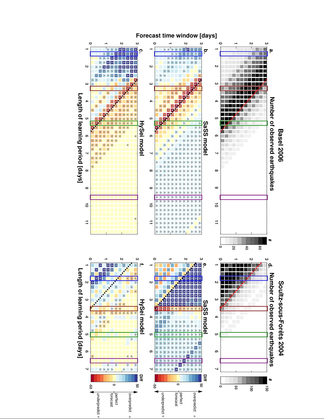
KIRAL Y-PR O A G ET AL.: V ALIDA TING INDUCED SEISMICITY F ORECAST MODELS X - 1 V alidating induced seismicit y forecast mo dels — Induced Seismicit y T est Benc h Eszter Kir´ aly-Proag 1 , J. Douglas Zec har 1 , V alen tin Gisc hig 2 , Stefan Wiemer 1 , Dimitrios Karvounis 1 , and Joseph Do etsc h 2 An edited version of this pap er w as published b y AGU. Copyrigh t (2016) American Geoph ysi- cal Union. Kir´ aly-Proag, E., J. D. Zec har, V. Gischig, S. Wiemer, D. Karvounis, and J. Do etsch (2016), V alidating induced seismicit y forecast mo dels — Induced Seismicit y T est Benc h, J. Geo- ph ys. Res. Solid Earth, 121, doi:10.1002/2016JB013236. T o view the published open abstract, go to h ttp://dx.doi.org and en ter the DOI. Corresp onding author: E. Kir´ aly-Proag, Swiss Seismological Service, ETH Zurich, NO H51.3, Sonneggstrasse 5, 8092 Zurich, Switzerland. (eszter.kiraly@sed.ethz.ch) 1 Swiss Seismological Service, ETH Zuric h, Zuric h, Switzerland. 2 Swiss Comp etence Cen ter for Energy Researc h (SCCER-SoE), ETH Zurich, Zuric h, Switzerland D R A F T D R A F T X - 2 KIRAL Y-PRO A G ET AL.: V ALID A TING INDUCED SEISMICITY FORECAST MODELS Key P oin ts. ◦ W e introduce a CSEP-based ob jectiv e test b ench for induced seismicity forecast mo dels. ◦ W e introduce a 3D smo othed seismicity mo del for induced earthquakes. ◦ W e compare forecast mo dels with diﬀerent ph ysical and statistical ele- men ts on t w o EGS reservoirs. Abstract. Induced earthquak es often accompan y ﬂuid injection, and the seismic hazard they p ose threatens v arious underground engineering pro jects. Mo dels to monitor and con trol induced seismic hazard with traﬃc ligh t sys- tems should b e probabilistic, forw ard-looking, and up dated as new data ar- riv e. In this study , w e prop ose an Induced Seismicity T est Benc h to test and rank suc h mo dels; this test b ench can b e used for mo del dev elopmen t, mo del selection, and ensemble mo del building. W e apply the test bench to data from the Basel 2006 and Soultz-sous-F or ˆ ets 2004 geothermal stim ulation pro jects, and w e assess forecasts from tw o mo dels: Shapiro and Smo othed Seismic- it y (SaSS) and Hydraulics and Seismics (HySei). These mo dels incorp orate a diﬀeren t mix of ph ysics-based elemen ts and sto chastic representation of the induced sequences. Our results sho w that neither mo del is fully sup erior to the other. Generally , HySei forecasts the seismicity rate b etter after shut- in, but is only medio cre at forecasting the spatial distribution. On the other hand, SaSS forecasts the spatial distribution b etter and giv es b etter seismic- it y rate estimates b efore sh ut-in. The sh ut-in phase is a diﬃcult moment for b oth models in b oth reserv oirs: the mo dels tend to underpredict the seismic- it y rate around, and shortly after, sh ut-in. D R A F T D R A F T KIRAL Y-PR O A G ET AL.: V ALIDA TING INDUCED SEISMICITY F ORECAST MODELS X - 3 1. In tro duction 1.1. Induced seismic hazard Seismicit y caused b y h uman activity , what is currently b eing called induced seismic- it y , is not a new phenomenon. Ov er the last sev eral decades, work ers ha v e noted that earthquak es are triggered b y h uman activities including n uclear explosions [ Boucher et al. , 1969], ﬂuid extraction [ Se gal l , 1989], ﬂuid injection [ Se eb er et al. , 2004; El lsworth , 2013], con trolled ﬁlling of artiﬁcial reservoirs (e.g., Koyna, India) [ Gupta , 2002], and mining and exca v ation [ McGarr , 1976]. But interest in induced seismicity has recently spiked, as has the rate of induced earthquakes in the central and eastern US [ El lsworth , 2013; Wein- garten et al. , 2015]. Here, it app ears that ﬂuid injections, primarily inv olving w astew ater, are causing extensive seismic activity including ev en ts suc h as the 2011 m w 4 . 0 earthquake in Y oungstown, Ohio, [ Kim , 2013], the 2011 m w 4 . 7 central Ark ansas earthquak e [ Horton , 2012], the 2011 m w 5 . 7 cen tral Oklahoma earthquak e [ Ker anen et al. , 2013], and the 2012 m w 4 . 9 east T exas earthquake [ F r ohlich et al. , 2014]. F or mo dern deep geothermal energy pro jects, induced seismicit y is a concern b ecause ﬂuids must b e injected to stim ulate and enhance reserv oir p ermeability , allowing the heat to b e ex tracted. There are tw o recen t examples in Switzerland: the Basel EGS exp erimen t in 2006 [ H¨ aring et al. , 2008] and the St. Gallen hydrothermal injection in 2013 [ Kr aft et al. , 2013; Edwar ds et al. , 2015; Ob ermann et al. , 2015]. Both pro jects were canceled: Basel b ecause of widely-felt seismic activity , and St. Gallen due to gas inﬂow, the lo w natural ﬂuid ﬂo w rate, and the high level of seismic activity during a short-term stimulation. These exp erimen ts demonstrated that pro ject managers and op erators hav e to b e able to manage induced seismic hazard and m ust strik e a balance b etw een reserv oir creation (i.e., D R A F T D R A F T X - 4 KIRAL Y-PRO A G ET AL.: V ALIDA TING INDUCED SEISMICITY FORECAST MODELS p ermeabilit y enhancemen t, whic h is required for a geothermal system to b e proﬁtable) and induced seismicity . Induced seismicity during geothermal pro jects is a blessing and a curse: the spatial extent of micro-seismicit y is a proxy for the size of the stim ulated reserv oir, but felt and p oten tially-damaging earthquak es p ose seismic risk to p eople and infrastructure. Induced earthquak es in deep geothermal reservoirs are usually smaller than m 3, but larger even ts ( > m 4) can o ccur, the largest so far b eing an m 4 . 6 earthquak e at the Geysers geothermal site in 1982 [ Majer et al. , 2007]. Certainly , induced earthquakes felt b y the public may deter future geothermal pro jects. Despite the cancellations at Basel and St. Gallen, sev eral geothermal pro jects in Switzerland are in dev elopmen t. As part of the Swiss national energy strategy , deep geothermal heat should supply 5 − 10% of the national baseload electricity [ Giar dini , 2014]. One of the main obstacles to achieving this goal is induced seismic hazard. T o minimize induced seismic hazard, it is crucial not only to monitor and analyze induced ev en ts, but also to develop a near-real-time to ol for making operational decisions. Suc h a hazard managemen t sc heme should b e used to plan and operate reservoir stim ulation so that large induced earthquak es are av oided [e.g., Bachmann et al. , 2011; Mena et al. , 2013; Go ertz-Al lmann and Wiemer , 2013]. 1.2. Near-real-time forecasting: to w ards an adaptive traﬃc light system Bommer et al. [2006] in troduced a traﬃc ligh t system to monitor and react to seismic activit y during geothermal reserv oir stim ulation. Lik e most traﬃc lights, this system distinguished three hazard lev els, which w ere based on the size of ev en ts, observ ed p eak ground v elo cit y , and public resp onse. But the thresholds used to c hange the light were c hosen sub jectively , primarily b y exp ert judgmen t [ Hirschb er g et al. , 2015], and in practice the system has resulted in op erators taking action to o late to a v oid large ev en ts or a high D R A F T D R A F T KIRAL Y-PR O A G ET AL.: V ALIDA TING INDUCED SEISMICITY F ORECAST MODELS X - 5 seismicit y rate. F or example, in Basel the early induced earthquak es suggested that felt ev en ts w ere likely , but the traﬃc ligh t system failed to anticipate them [ H¨ aring et al. , 2008]. An impro v ed hazard managemen t scheme should b e a dynamic, forw ard-looking system that incorp orates real-time data and makes probabilistic forecasts of induced seismicit y and its consequences. Such an Adaptive T raﬃc Ligh t (A TL) system is comp osed of several mo dules (Figure 1): 1. Collecting prior information, e.g., geological setting for hazard assessmen t and build- ing classiﬁcations for risk assessmen t (y ellow in Figure 1). These data are essen tial to plan a geothermal pro ject and can address questions such as where to drill wells, the orien- tation of the lo cal stress ﬁeld, ho w to design reserv oir creation plans, and the maxim um p ossible magnitude [ Gischig , 2015]. 2. Real-time data ﬂow of h ydraulic and seismic information (red in Figure 1). These are h ydraulic data (e.g., injection ﬂow rate and pressure measuremen ts in the w ell) and seismic data that allow one to monitor reservoir creation, circulation, or other activities in the reserv oir. 3. Modeling and forecasting seismicit y (orange in Figure 1). The key elemen t in an A TL system is seismicit y forecasting. T o forecast, we consider tw o p erio ds: a learning p erio d and a forecast p erio d. During the learning perio d, seismic even ts are observ ed and analyzed according to their distribution in time and space. Then a calibrated model forecasts the num b er, magnitude distribution, and spatial distribution of even ts in the forecast p erio d. 4. Ground motion mo dels (gra y in Figure 1). These mo dels estimate the shaking that an earthquake will cause and are based on prop erties of the earthquake source (e.g., D R A F T D R A F T X - 6 KIRAL Y-PRO A G ET AL.: V ALIDA TING INDUCED SEISMICITY FORECAST MODELS its magnitude, st yle of faulting, and depth), wa ve propagation (distance to the earth- quak e), and site resp onse (t yp e of ro ck, soil that can attenuate or amplify ground shaking). Ground Motion Prediction Equations [ Douglas et al. , 2013] and the Virtual Earthquake Approac h [ Denol le et al. , 2013, 2014] are examples of possible choices to estimate ground motions. 5. Com bining mo dels to account for epistemic uncertain ties (green in Figure 1). No single model captures all of the imp ortant features of seismicit y . Mo del combination using appropriate weigh ts is one w a y to try to leverage eac h mo del’s b est features. 6. Calculating hazard and risk (bro wn in Figure 1). One can estimate the seismic haz- ard — the probabilit y that some lev el of shaking will be exceeded — b y com bining ground motion mo dels and either syn thetic catalogs generated b y forecast models or individual scenario earthquak es. One can use this hazard to estimate the seismic risk: the potential economic, so cial, and environmen tal consequences of seismicit y . 7. Guiding on-site decision-making pro cesses (white in Figure 1). Based on hazard and risk calculations, op erators can mak e decisions concerning future stimulation strategies and adjust ﬂo w rate accordingly . In this pap er, we fo cus on the forecast mo dels and the p erformance assessment mo dules of the A TL system (delineated by a dashed gra y line in Figure 1). 1.3. Mo dels to forecast seismicit y Induced seismicity mo dels can b e group ed in to three classes [e.g., Gischig and Wiemer , 2013; Gaucher et al. , 2015]: statistical, ph ysics-based, and h ybrid. In general, statistical mo dels for induced seismicit y [e.g., R e asenb er g and Jones , 1989; Hainzl and Ogata , 2005; Bachmann et al. , 2011; Mena et al. , 2013] are conceptually and computationally simple D R A F T D R A F T KIRAL Y-PR O A G ET AL.: V ALIDA TING INDUCED SEISMICITY F ORECAST MODELS X - 7 and include aleatory uncertaint y . But they do not explicitly accoun t for the ph ysical pro cesses go v erning induced seismicit y (e.g., ﬂuid ﬂo w in fractures, p ermeability changes, and stress in teraction) and, un til this study , they hav e not b een used to forecast the spa- tial distribution of earthquak es. It is sometimes though t that statistical mo dels, b ecause they are primarily based on clustering, are limited in their ability to predict large ev en ts or mak e accurate long-term forecasts. In contrast, physics-based mo dels [e.g., Olivel la et al. , 1994; Bruel , 2005; Kohl and M ´ egel , 2007; Baisch et al. , 2010; Rinaldi et al. , 2015; McClur e and Horne , 2012; Wang and Ghassemi , 2012; Karvounis and Wiemer , 2015; Mignan , 2015] do consider underlying ph ysical pro cesses, and are hop ed to perform b et- ter when op erational conditions change, such as for the sh ut-in p erio d, and for long-term forecasts. But the high computational exp ense of most ph ysics-based mo dels precludes their use in near-real-time applications for the moment. Hybrid models are a compromise b et w een physical mo dels and statistical models. The goal of h ybrid model developmen t is to include some ph ysical complexity and replace more complex ph ysical considerations with statistical metho ds or sto c hastic pro cesses. Mena et al. [2013] compared forecast mo dels using the Basel dataset and found that Shapiro’s mo del [ Shapir o et al. , 2010] provided a go o d ﬁt to the rate of induced earth- quak es. This mo del uses the seismogenic index, Σ, a parameter that describ es the exp ected seismic resp onse of a giv en site. The seismogenic index is a function of the total injected ﬂuid v olume and can b e estimated from a short injection p erio d or from the entire stim- ulation p erio d; it also tak es in to accoun t the b -v alue of the observed seismicity and the total injected v olume. Using Σ, one can forecast the n um ber of earthquak es in a given magnitude range and giv en p erio d. Like most statistical mo dels for induced seismicity D R A F T D R A F T X - 8 KIRAL Y-PRO A G ET AL.: V ALIDA TING INDUCED SEISMICITY FORECAST MODELS [e.g., Bachmann et al. , 2011], Shapiro’s mo del do es not make any predictive statements ab out the size or shap e of the seismicit y cloud. But it is crucial to monitor and anticipate the shap e and size of the seismic cloud during reservoir stim ulation for t w o reasons. First, the extent of the seismicity cloud is used to estimate the v olume of the stim ulated reser- v oir, whic h is crucial for energy pro duction. Second, the spatial distribution of seismicit y aﬀects hazard and risk analysis: many geothermal sites are lo cated near settlemen ts, mak- ing energy transp ortation c heap but p osing a risk to infrastructure and p eople [ Edwar ds et al. , 2015]. Seismic risk strongly dep ends on geological settings (e.g., ro c k t ype under the settlement), building vulnerabilit y , and the depth of induced ev en ts. F or instance, if a m w 4 ev en t o ccurs 5 k m b elow strong, new homes built on a ro ck site, almost all buildings w ould remain in tact, with only some slight damage. If an ev en t of the same size occurs 3 k m b elo w vulnerable houses built on a sedimen tary basin, it is more lik ely that the houses would b e slightly damaged, and some houses may b e mo derately or ev en heavily damaged [ Gr ¨ unthal , 1998]. Because the spatial distribution of induced seismicity is so imp ortan t, any A TL system should b e driv en by 3D spatial forecasts. In this study , ﬁrst w e extend Shapiro’s model to pro duce 3D forecasts (SaSS mo del, i.e., Shapiro and Smo othed Seismicity mo del). Then, we p erform systematic statistical tests on this mo del and on a h ybrid mo del, in which seismicit y is triggered b y a n umerically mo deled pressure diﬀusion (HySei mo del, i.e., Hydraulics and Seismicit y mo del). T o date these are the only mo dels in our institute, that are calibrated against real data, and systematic re-calibration and testing can b e carried out; moreov er, they ha v e a go o d v ariety of mo del features, whic h forecasts are w orth ev aluating and comparing. T o do this, we dev elop an Induced Seismicity T est Bench. D R A F T D R A F T KIRAL Y-PR O A G ET AL.: V ALIDA TING INDUCED SEISMICITY F ORECAST MODELS X - 9 1.4. Induced Seismicit y T est Bench Little w ork has b een done on model selection and mo del comparison in the context of induced seismicit y . T o v alidate, compare, and rank models that can b e used for A TL systems, w e prop ose a mo del dev elopmen t test bench that follo ws the Collab oratory for the Study of Earthquak e Predictabilit y (CSEP , http://www.cseptesting.org/) approac h for tectonic earthquak es. CSEP supp orts scien tiﬁc earthquake prediction exp eriments in natural lab oratories in multiple regions and spanning the glob e [e.g., Gerstenb er ger and R ho ades , 2010; Schorlemmer et al. , 2010; Ze char et al. , 2010a; Nanjo et al. , 2011; Eb erhar d et al. , 2012; Mignan et al. , 2013; T ar oni et al. , 2013; Ze char et al. , 2013]. This supp ort comes in the form of testing cen ters that CSEP op erates; these cen ters allo w mo delers to c hec k the consistency of their mo del with observ ations and to compare mo dels. W e describ e these activities in more detail in Subsection 3.2. The prop osed Induced Seismicity T est Benc h requires mo dels to b e tested, go o d qualit y induced seismicit y datasets, and a robust statistical testing framew ork allowing ob jective mo del ev aluation. T o test mo del consistency with observ ations and to rank mo dels, w e rely on pseudo-prospective forecasting, i.e., data that come from past stim ulation exp eriments. Mo delers calibrate their mo dels using data recorded during a learning p erio d and make forecasts for a subsequen t forecast p erio d. Since observed data of the forecast p erio ds are already a v ailable, we can compare observed and forecast data after eac h recalibration and test the consistency of the forecast in terms of seismicit y rate, spatial distribution, and magnitude distribution. W e can use statistical metrics suc h as the information gain p er earthquak e to compare mo del pairs and rank mo dels according to their forecast skill [ R ho ades et al. , 2011]. Mo delers should use the results of testing for further dev elopmen t, D R A F T D R A F T X - 10 KIRAL Y-PR O A G ET AL.: V ALIDA TING INDUCED SEISMICITY F ORECAST MODELS creating a feedback b etw een testing and mo deling. The long-term goal is to dev elop an op erational A TL system to plan and conduct reservoir creation without a high rate of seismicit y or large even ts. A detailed ﬂo w c hart of the Induced Seismicit y T est Bench can b e found in the supplemen t (Figure S1). The Induced Seismicity T est Bench is a diagnostic to ol: it can highligh t which mo del ele- men ts, b e they ph ysical or statistical, are essen tial for go o d forecasts, and wh y . This can in turn impro v e the models and our understanding of the underlying physical phenomena. In addition to using the test b ench as a diagnostic to ol, it can also b e utilized on the ﬂy to judge the p erformance of sev eral mo dels since the last forecast. The results can then b e used for further improv emen t of the individual mo dels and/or they can be applied to w eigh t the mo dels for the next forecast. In the next section, we brieﬂy describ e the data from t w o Enhanced Geothermal Sys- tems: the Basel 2006 exp eriment and the Soultz-sous-F orˆ ets 2004 stim ulation. In Section 3 w e presen t t w o mo dels, SaSS (Shapiro and Smo othed Seismicity) model and HySei (Hydraulics and Seismicit y), which are calibrated on the datasets; and w e also detail the testing approach. W e describ e the testing results in section 4, discuss our ﬁndings in section 5, and conclude in section 6. 2. Data The data w e consider in this study come from the Soultz-sous-F orˆ ets 2004 and Basel 2006 geothermal stim ulations. The Basel geothermal site is lo cated in north w estern Switzerland, at the southeastern part of the Upp er Rhine Grab en (Figure 2.a). The graben structure is an inactiv e extensional rift system oriented N-S [ Zob ack , 1992]. Here, the crystalline basemen t is cov ered b y D R A F T D R A F T KIRAL Y-PR O A G ET AL.: V ALIDA TING INDUCED SEISMICITY F ORECAST MODELS X - 11 2 . 4 k m of sedimentary ro c k [ H¨ aring et al. , 2008]. The w ell BASEL1 w as drilled to a depth of 5 k m betw een Ma y and Octob er 2006. In Decem b er 2006, after sev eral h ydraulic tests, the reserv oir was h ydraulically stimulated to enhance its p ermeability . The plan was to stim ulate for 21 da ys, but after 6 days the injection was stopp ed due to intensiv e seismicity . In the year that follo w ed, 3 additional even ts of m L > 3 . 0 follow ed [ H¨ aring et al. , 2008]. Based on the results of a subsequent risk study [ Baisch et al. , 2009; Se c anel l et al. , 2009], the pro ject w as abandoned. After several years, the reserv oir still has earthquak es, but the seismicity rate is very lo w (1-3 earthquak es recorded p er year) [ Deichmann et al. , 2014]. In this study , we use ab out 15 da ys of h ydraulic [ H¨ aring et al. , 2008] and seismic data [ Dyer et al. , 2010] from the b eginning of the stimulation (2006-12-02, 18:00), and w e also use the pre-stimulation injection test data. The Soultz-sous-F orˆ ets geothermal site is also lo cated in the Upp er Rhine Grab en, b etw een Kutzenhausen and Soultz-sous-F or ˆ ets, ab out 70 km north of Strasbourg (Alsace, F rance; inset in Figure 2). The geothermal gradient is ab out 100 ◦ C /k m within the 1 . 5 k m thic k sedimen tary cov er ov er a granitic basement [ Evans et al. , 2012]. This abnormally high geothermal gradient is related to deep h ydrothermal conv ection cells in the fractured basemen t [ G´ er ar d et al. , 2006]. The geothermal pro ject here started in the early 1980s and four wells ha v e b een drilled in to t w o reservoirs: one at ab out 3 . 5 k m depth (GPK1, GPK2 w ells) and another at ab out 4 . 5 km (GPK2, GPK3, GPK4 w ells). Several stimulations and circulation tests w ere carried out [ G´ er ar d et al. , 2006; Cal` o et al. , 2014; Genter et al. , 2012]. Energy pro duction started in 2008 [ Genter et al. , 2010]. In this study , we use hydraulic and seismic data of the pre-stimulation and stim ulation of Septem b er 2004 (Figure 2.b, Dyer [2005]). Lo cal magnitudes were corrected b y using the scaling relationship b y Douglas D R A F T D R A F T X - 12 KIRAL Y-PR O A G ET AL.: V ALIDA TING INDUCED SEISMICITY F ORECAST MODELS et al. [2013]. Note that the seismograms in this data set are clipped, causing saturation of the magnitudes at 1 . 8; that is, no ev en t has m w > 1 . 8. 3. Mo dels and testing 3.1. The Shapiro and Smo othed Seismicit y (SaSS) mo del The SaSS mo del is computationally simple and based on the seismogenic index, Σ [ Shapir o et al. , 2010]; we distribute the earthquak es exp ected b y Σ in 3D b y smo othing seismicit y in space. Shapiro’s mo del, whic h describ es the rate of induced seismicity during stim ulation, is deﬁned as: l og 10 ( N m ( t )) = l og 10 ( Q c ( t )) − bm − Σ (1) where N m ( t ) indicates the num ber of induced ev en ts ab ov e magnitude m up until time t , Q c ( t ) denotes the cum ulativ e injected v olume of ﬂuid at time t , b is Guten berg-Rich ter b -v alue of the observed seismicity , and m is the magnitude ab ov e which all even ts are exp ected to b e reliably recorded (often called the magnitude of completeness). T o forecast the num ber of even ts in the forecast p erio d, w e estimate Σ and b from the learning p erio d, and w e predict the total volume that will b e injected b y the end of the forecast perio d. Kir´ aly et al. [2014] compared four deep geothermal datasets and found that in some cases b and Σ are not constant during and after stim ulation; th us, we re- estimate them at the end of each learning p erio d, ev ery six hours. T o predict Q c ( t ) at the end of a forecast p erio d, w e assume that the injection ﬂo w during the forecast p erio d will follo w the previously-planned strategy . Eq. 1 describes the rate of induced seismicit y only during stimulation [ Shapir o et al. , 2010]. As soon as the stim ulation stops (the momen t of w ell sh ut-in), the rate of induced earthquakes is exp ected to decay; the SaSS mo del D R A F T D R A F T KIRAL Y-PR O A G ET AL.: V ALIDA TING INDUCED SEISMICITY F ORECAST MODELS X - 13 assumes the decay follows the equation of L angenbruch and Shapir o [2010] (using the original notation for consistency): R 0 b  t t 0  = R 0 a  t t 0  p (2) where R 0 b is the p ost-stimulation seismicit y rate at time t (since the b eginning of the stim ulation), t 0 is the length of the stimulation p erio d b efore shut-in, R 0 a denotes the a v- erage seismicity rate during stim ulation, and p controls ho w quickly the rate deca ys. F or subsequen t forecast time windows (i.e., 6-hour time bins of the forecast p erio d, FTWs), the ma jorit y of parameters are calibrated on the corresp onding learning p erio d, but Q c and R b 0 are recalculated for eac h time windo w. If the learning perio d ends in the stimula- tion p erio d but some FTWs expand to the p ost-stim ulation, the estimation of parameter p is not p ossible, thus w e use a generic v alue: p = 2. Also, if p is estimated to b e smaller than 2 w e set the v alue to 2, follo wing the v alue that is prop osed b y L angenbruch and Shapir o [2010] for an early p ost-injection p erio d. Detailed ﬂo w c hart of num ber comp onen t can b e found in the supplemen t (Figure S2). As in CSEP experiments and suggested by Shapir o et al. [2010], the n um ber of even ts in each forecast p erio d is assumed to follow a P oisson distribution and the n um bers obtained by using Eq. 1 and 2 are Poisson expected v alues; error bars in all subsequen t ﬁgures indicate the 95% P oisson conﬁdence in terv al. T o mo del the 3D spatial distribution of induced earthquakes, w e added a spatial compo- nen t to the mo del by smo othing the seismicit y observed during the learning p erio d (Fig- ure 3.A). Sev eral studies, including the Regional Earthquak e Likelihoo d Mo dels (RELM) exp erimen t [ Schorlemmer et al. , 2010; Ze char et al. , 2013] hav e shown that smo othed seismicit y mo dels are eﬀective at forecasting the spatial distribution of tectonic earth- D R A F T D R A F T X - 14 KIRAL Y-PR O A G ET AL.: V ALIDA TING INDUCED SEISMICITY F ORECAST MODELS quak es. T o construct a smo othed seismicit y mo del in t w o dimensions, one applies a tw o- dimensional smo othing kernel to each past ev en t [e.g., Helmstetter et al. , 2007], calculates the contribution of smo othed earthquakes on a given grid, then sums con tributions of all observ ed earthquak es. T o create a probability density function (PDF, i.e., earthquake spatial probability map), one normalizes the smo othed seismicit y map so its sum is unity . W e extend the 2D Gaussian smo othed seismicit y mo del of Ze char and Jor dan [2010] to 3D. F or each forecast p erio d, we smo oth all prior ev en ts, where the contribution of an earthquak e to a given v o xel (i.e., volume elemen t) is K ( x e , y e , z e , x 1 , x 2 , y 1 , y 2 , z 1 , z 2 ) = 1 8 " er f  x 2 − x e σ 1 √ 2  − er f  x 1 − x e σ 1 √ 2  # × " er f  y 2 − y e σ 2 √ 2  − er f  y 1 − y e σ 2 √ 2  # × " er f  z 2 − z e σ 3 √ 2  − er f  z 1 − z e σ 3 √ 2  # (3) where x e , y e and z e denote the lo cation of the given earthquak e, x 1 , x 2 , y 1 , y 2 , z 1 and z 2 are the p oints that deﬁne the edges of the v o xel, and σ 1 , σ 2 and σ 3 are bandwidths of the 3D Gaussian k ernels in EW, NS and v ertical directions, resp ectiv ely . T o make a go o d smo othed seismicity forecast, w e need go o d bandwidths; w e optimize these by dividing data from the curren t learning perio d into a training set and a v alidation set (Figure 3.C). The length of the training and v alidation sets dep end on the length of the forecast p erio d and the learning p erio d. If the length of the forecast perio d is more than half the length of the learning p erio d, the training and v alidation sets are eac h one-half of the learning p erio d. Otherwise, the length of the v alidation set is equal to the length of the forecast p erio d. W e searc h for the bandwidth com bination that, when used to smo oth the training D R A F T D R A F T KIRAL Y-PR O A G ET AL.: V ALIDA TING INDUCED SEISMICITY F ORECAST MODELS X - 15 set, b est forecasts the seismicity of the v alidation set. T o a v oid ’surprises,’ i.e., ev en ts o ccurring where the model would not exp ect any even ts, w e distribute a certain fraction of the PDF o v er all vo xels (i.e., surprise factor), following the idea of Kagan and Jackson [2000]. W e analyze the p erformance of 1000 com binations of bandwidths and surprise factors using the training and v alidation set of the learning p erio d. The PDF is up dated for eac h new learning/forecast perio d. Since the PDF is based on the learning p erio d, this mo del assumes that earthquak e lo cations in the forecast p erio d will not b e v ery diﬀeren t from the seismicit y observed so far. Smo othed induced seismicity mo dels m ust diﬀer from their tectonic coun terparts in at least one asp ect: induced mo dels should capture the propagation of the seismicit y front after sh ut-in. In particular, due to pore pressure diﬀusion, induced seismic activity tends to decrease in the vicinity of the injection well and to concen trate at the b oundaries of the reserv oir. W e attempt to mo del this time-dep endent eﬀect b y applying exponential temp oral weigh ting: the most recent ev en t receiv es a maxim um w eigh t (one), and earlier ev en ts get smaller weigh ts according to their origin time. This is analogous to the ex- p onen tial smo othing approac h commonly used in time series forecasting [ Go o dwin , 2010] and is also connected to the Omori-Utsu relation describing aftershock decay rate [ Zhuang et al. , 2012]. The forecast magnitude distribution is the Gutenberg-Rich ter distribution [ Gutenb er g and Richter , 1944] with the b -v alue estimated from the learning perio d. 3.2. The Hydraulics and Seismicit y (HySei) mo del The HySei mo del dev eloped by Gischig and Wiemer [2013] describ es seismicity triggered b y pressure diﬀusion with irrev ersible p ermeability enhancemen t. The biggest adv an tage D R A F T D R A F T X - 16 KIRAL Y-PR O A G ET AL.: V ALIDA TING INDUCED SEISMICITY F ORECAST MODELS of the mo del is that it quantiﬁes p ermeabilit y enhancemen t b y calibrating ﬂow rate and w ellhead pressure against observ ations. The HySei mo del consists of t w o main parts: h ydraulic in v ersion and seismicit y mo deling. The aim of in v erting hydraulic observ ations is to reconstruct the pressure evolution in the reserv oir. W e seek the b est h ydraulic parameters to matc h the observ ed w ell-head pressure with a one-dimensional radial ﬂow mo del. W e use a ﬁnite diﬀerence metho d in a circle of 1200 m radius distributed on 3000 no des, and 1-minute resolution in time. During the pre-stim ulation test injection, w e solv e the diﬀusion equation (Eq. 4) with constan t p ermeabilit y ( κ = κ 0 ). During stimulation the go v erning equations are the diﬀusion equation (Eq. 4) with irrev ersible c hanging p ermeabilit y (Eq. 5) due to increasing pressure that exceeds some threshold (Eq. 6): ρS ∂ p ∂ t = ∇  κρ µ ∇ p  + q m (4) κ = κ 0 ( u + 1) (5) ∂ u ∂ t = C u H pt  ∂ p ∂ t  H u ( u t − u ) H p ( p − p t ) (6) where ρ is ﬂuid density , S is the sp eciﬁc storage co eﬃcient, κ is p ermeability that v aries during the stim ulation, µ is ﬂuid viscosity , and q m is a mass source; κ 0 is the initial p ermeabilit y b efore the stimulation, u is stimulation factor (i.e., the ov erall p ermeabilit y enhancemen t of the reserv oir); C u is stim ulation v elocity , a constan t that scales the rate at whic h p ermeabilit y changes, u t is maxim um stim ulation factor, and p t is threshold pressure, H pt is a Hea viside function, it is one if pressure increases, zero otherwise, H p and H u are Hea viside functions for pressure and stimulation factor. These are smo othed D R A F T D R A F T KIRAL Y-PR O A G ET AL.: V ALIDA TING INDUCED SEISMICITY F ORECAST MODELS X - 17 to a v oid a singularit y and resulting n umerical instability . Permeab ilit y starts to increase if pressure reac hes p t . If pressure further increases, the p ermeabilit y of the reserv oir increases un til it reac hes u t . Note that a reversible comp onent of permeability c hange representing the complian t resp onse fracture to pressurization [e.g., Rutqvist and Stephansson , 2003] has not b een included in this v ersion of the mo del. In the seismicit y mo del, randomly-placed p otential n ucleation p oints are triggered b y the radial symmetric pressure evolution following the Mohr-Coulom b failure criterion. They hav e no spatial extent, but diﬀerential stress ( σ 1 − σ 3 ) is deﬁned at the seed p oint. Lo cal b -v alues are determined at the seed p oin ts follo wing a linear relationship b et w een diﬀeren tial stress and b -v alue: b max and b min parameters are b -v alues at minimum and max- im um v alues of diﬀeren tial stress, resp ectiv ely . When a seed p oin t is triggered, a random magnitude is dra wn from the magnitude distribution with the lo cal b -v alue. Additional free parameters are the scaling factor F s (the ratio b etw een the n um ber of synthetic and observ ed even ts), the stress drop co eﬃcien t dτ (the change of stress conditions after a seed has been triggered), and a criticality threshold dµ , whic h accoun ts for the fact that seed p oints cannot b e to o close to the failure limit. F or this study , we parallelized parts of the co de and extended the model to 3D (Figure 3.B) by adding an oﬀ-fault comp onen t to the originally 2D seismicit y mo del. Assuming that the seismicity is generated on the curren t main fault, we determine the principal comp onen ts of the curren t seismicit y cloud and use the empirical distribution of the seis- micit y along the smallest axis to deﬁne oﬀ-fault co ordinates of the syn thetic even ts. A detailed ﬂow c hart of the HySei mo del can b e found in the supplement (Figure S3). T o represent the spatial diﬀerences of the tw o mo dels, Figure 4 shows cross sections of D R A F T D R A F T X - 18 KIRAL Y-PR O A G ET AL.: V ALIDA TING INDUCED SEISMICITY F ORECAST MODELS the 3D PDFs of SaSS (upp er line) and HySei (b ottom line) at the momen t and location of the biggest even t ( m w = 3 . 1), which o ccurred about 5 hours after the sh ut-in. 3.3. T esting T o assess a single model, w e chec k if its forecasts are consistent with the observ ations [ Ze char et al. , 2010b], asking the question: migh t the observ ations hav e b een generated b y this mo del? One wa y we do this is to chec k if the num ber of observed earthquakes falls within the 95% conﬁdence interv al of the forecast. If so, the mo del passed the Num b er-test. In a similar wa y , w e examine if the magnitude distribution of all forecasts is consisten t with the observ ations (Magnitude-test). T o test the spatial comp onent (Space- test) [ Ze char et al. , 2010b; R ho ades et al. , 2011], w e use a testing grid of 4 km × 4 k m × 4 k m cen tered on the well tip and divided in to 200 m × 200 m × 200 m v o xels. After normalizing the forecasts so that the n um ber of forecast ev ents matches the n umber of observed even ts, w e calculate the log-likelihoo d (LL) of the observ ation in eac h vo xel. Summing these v alues giv es a joint LL for a sp eciﬁc exp eriment. The higher the join t LL v alues are the b etter the forecast [ Ze char et al. , 2010b; R ho ades et al. , 2011]. T o chec k if the forecast is consisten t with the observ ed seismicit y of the forecast p erio d, w e sim ulate 1000 catalogs from the forecast, and ﬁnd the 5 th p ercen tile of the LL v alues for the simulated catalogs. If the LL for the current observ ation is higher than the 5 th p ercen tile the forecast passed the Space-test — the observ ed seismicity could hav e b een generated by the mo del. Both mo dels consider the earthquake distribution Poissonian, th us LL v alues are calculated as follo ws: D R A F T D R A F T KIRAL Y-PR O A G ET AL.: V ALIDA TING INDUCED SEISMICITY F ORECAST MODELS X - 19 L ( A ) = n X i =1 h k i × l og  λ A i  − λ A i − l og  k i !  i (7) where L ( A ) is the Poisson joint LL of forecast A, n is the n um ber of v o xels, k i is the n um ber of earthquakes observed in the ith v o xel, and λ A i is the forecast seismicit y rate in the i th v o xel of forecast A. T o compare t w o mo dels, one can directly compare individual LL v alues of the mo dels either for mo del comp onen ts (i.e. ev en t num bers, magnitudes or the spatial component) separately or for the en tire mo del. These measures give information ab out the mo del p erformance not only against data but against other mo dels. Here w e would lik e to emphasize that LL v alues consider the whole mo del space. In other w ords, it reﬂects the p erformance of not only the temp oral/magnitude/spatial bins that host at least one earthquak e but also the empty ones answering the question: what is the probability to ha v e zero earthquake in the giv en temp oral/magnitude/spatial bin? One can also calculate the information gain of one mo del with resp ect to another for mo del comparisons. This measure emphasizes the non-empt y bins b y comparing the forecast seismicit y rates of mo del A with that of mo del B in the vo xels where earthquak es o ccurred. The follo wing form ula gives I i , the information gain of mo del A o v er mo del B for an earthquak e o ccurring in the i th v o xel [ R ho ades et al. , 2011]: I i = − N A + N B N + l n λ A i λ B i ! (8) where N is num ber of observ ed ev en ts, λ A i and λ B i denote forecast seismicit y rate in the i th v o xel of mo del A and B , resp ectiv ely , N A and N B are the total forecast num b er of ev en ts in mo del A and B , resp ectiv ely . The ﬁrst term of the right hand side is a D R A F T D R A F T X - 20 KIRAL Y-PR O A G ET AL.: V ALIDA TING INDUCED SEISMICITY F ORECAST MODELS p enalt y concerning the n um b er of even ts under each model. W e seek to kno w if one mo del is b etter than the other, in other words, if the exp ected v alue of the information gain p opulation diﬀers from zero. One can also estimate how m uc h b etter or worse mo del A relative to mo del B (i.e., a v erage information gain) by ﬁnding an appropriate estimator. Exp onen tiating the a v erage information gain yields the a v erage probabilit y gain of mo del A with resp ect to mo del B . Additionally , 95% conﬁdence interv al of the estimated exp ected v alue can b e calculated to determine if mo del A is signiﬁcantly b etter or worse than mo del B : if the conﬁdence interv al con tains zero, the diﬀerence b etw een the mo dels is not statistically signiﬁcant at the 5% signiﬁcance lev el. Sev eral tec hniques are p ossible to compute the av erage information gain. Rho ades et al. [2011] suggested to take the arithmetic mean of the information gain distribution as the exp ected v alue of the p opulation, based on Studen ts t-distribution [ Student , 1908]. W e refer to this metho d as ’Classical mean’. This estimator is b est if the p opulation follo ws a normal distribution. Plotting the distribution of information gains (that is, for individual earthquakes) for SaSS relative to HySei as a function of time and in a quan tile- quan tile plot (Figure S4) suggests that the information gains are not normally distributed. One p ossible wa y to solve this problem is to seek an estimator that can tac kle outliers systematically . This can b e done by manual data screening and remov al of outliers, but it can b e impractical due to the large num ber of data p oin ts and p ossible masking (i.e., large outliers can hide smaller ones). T o o v ercome these problems, w e use robust statistics to automatically detect and do wn w eight outliers [ R uckstuhl , 2014]. W e refer to this metho d as ’Robust mean’. T o calculate the exp ected v alue of the information gain distribution, we compute a w eigh ted mean where the inﬂuence of the outliers is reduced. D R A F T D R A F T KIRAL Y-PR O A G ET AL.: V ALIDA TING INDUCED SEISMICITY F ORECAST MODELS X - 21 In particular, we use the Hub er M-estimator, implemented as mlo chub er in the LIBRA matlab pac k age [ V erb oven and Hub ert , 2005]. By using the Hub er M-estimator, w e a v oid the problem that a few earthquakes dominate the estimate of the av erage information gain. W e also explore a non-parametric metho d: generate 1000 b o otstrap samples of the observ ed information gains (i.e., we sample with replacement) and ﬁnd the arithmetic a v erage and 2 . 5% and 97 . 5% p ercentiles, thus obtaining a ”Bo otstrap mean” and the corresp onding 95% conﬁdence interv al. Using the same b o otstrap samples w e also ﬁnd ’Bo otstrap median’. W e show a comparison of these metho ds in the next section. 4. Results 4.1. Consistency tests Figure 5 sho ws four snapshots of forecast and observ ed seismicit y rates for b oth datasets. The top ro w sho ws the corresponding h ydraulic data (injection rate and w ell-head pres- sure) to provide time reference for the forecasts. Blue, red, green, and purple v ertical lines indicate the end of the diﬀeren t learning p erio ds: corresp onding shaded areas show forecasts of SaSS model (middle row) and HySei mo del (b ottom ro w) with 95% Poisso- nian conﬁdence interv als. In case of Basel 2006, b oth mo dels seriously ov erpredicts the seismicit y rate for LP1 (blue learning p erio d that ends at day 1 . 25). This migh t b e due to the short learning perio d. Giving longer learning p erio d to the mo dels (LP2, red learning p erio d that ends at da y 3 . 25), the forecast is greatly improv ed for b oth mo dels. SaSS struggles to forecast after b oth LP3 (green learning p erio d that ends at da y 5 . 25) and LP4 (purple learning p erio d that ends at day 9 . 5), while HySei underpredicts after LP3 and giv es p erfect forecast after LP4. In the case of Soultz-sous-F orˆ ets 2004, SaSS giv es go o d forecasts at ﬁrst (after LP1, the learning perio d that ends at da y 1 . 75), then sev erely D R A F T D R A F T X - 22 KIRAL Y-PR O A G ET AL.: V ALIDA TING INDUCED SEISMICITY F ORECAST MODELS underpredicts (after LP2 the learning perio d that ends at day 3 . 5), and ﬁnally signiﬁca n tly o v erpredicts the seismicity rate (after LP3 and LP4, the learning perio ds that end at da y 5 and 6 . 5, resp ectively). HySei p erforms w ell in most of the cases (after LP2, LP3 and LP4), except after LP1. In this case, the mo del exp ects higher pressure in resp onse to the injection p eaks b et w een da y 2 − 3, which results in ov erprediction of the sesimicity rate. This might b e due to the fact that a rev ersible component of p ermeabilit y c hange, p ossibly arising from fracture compliance, is not included in this v ersion of the mo del. T o sho w forecasts corresp onding to all learning p erio ds, w e use a matrix represen tation where colors indicate the goo dness of the forecast (Figure 6): y ello w means a p erfect fore- cast; red and blue mean under- or o v erprediction, resp ectiv ely . Down w ard- and upw ard- p oin ting triangles denote momen ts when the observ ed seismicity rate falls out of the 95% conﬁdence in terv als due to serious under- or o v erprediction, resp ectively . T o av oid ov erlap of the forecast perio ds, we represen t the 3-da y forecast p erio d vertically: the end of the learning perio d is indicated on the horizon tal axis, time during the 3-da y forecast p erio d is indicated on the vertical axis with subsequen t 6-hour FTWs. Time in the forecast p erio d increases from b ottom to top. The top ro w of Figure 6 shows the observed seismicity rate for both datasets, middle and bottom ro ws sho w a comparison of observ ed seismicity rates with forecasts from SaSS and HySei, resp ectively . In Basel, b oth models mainly o v eres- timate the n um b er of observed earthquak es during the initial stim ulation p erio d. When the injection rate w as decreased and at shut-in, both mo dels hav e diﬃculties forecasting the right num b er of earthquakes: they sev erely underpredict the observed seismicity rate. The SaSS mo del o v erpredicts for the p ost-stimulation p erio d, whereas HySei seems to ﬁnd go o d estimates most of the time for later p erio ds (with the exception of three time win- D R A F T D R A F T KIRAL Y-PR O A G ET AL.: V ALIDA TING INDUCED SEISMICITY F ORECAST MODELS X - 23 do ws). In Soultz-sous-F orˆ ets 2004, the SaSS mo del mainly forecasts well or o v erestimates the num ber of earthquak es during stim ulation. The forecast p erio d corresp onding to the learning p erio d of day 3 . 5 stands out, when SaSS signiﬁcantly underpredicted the num b er of earthquak es. This is b ecause there is not yet enough data of the p ost-injection p erio d to estimate p ost-stimulation parameters. During the p ost-stimulation p erio d, the SaSS mo del o v erpredicts almost all FTWs. On the other hand, the HySei mo del gives generally go o d results: there are only a few under- and ov erpredictions, mainly at the b eginning of the injection, around sh ut-in, and near the end of the in v estigated p erio d. Overall, in most of the cases, HySei is b etter at forecasting the num b er of induced earthquakes; this is reﬂected by the n um ber of unmark ed FTWs in Figure 6. Moreo v er, for a small perio d of re-injection in Soultz-sous-F orˆ ets (at da y 8), HySei forecasts the num b er of even ts w ell, while the SaSS mo del signiﬁcan tly ov erpredicts. In Figure 7 w e compare the observed magnitude distribution with forecasts from SaSS and HySei. Magnitude bins are 0 . 1 units wide and range from 0 . 9 to 4 for Basel 2006 and from 0 to 1 . 9 for Soultz-sous-F orˆ ets 2004. W e remind the reader that the Soultz-sous- F or ˆ ets 2004 magnitudes are truncated, so the ﬁnal magnitude bin contains all ev en ts that w ould ha v e m > 1 . 8. Both mo dels forecast the magnitude distribution of micro-seismic ev en ts w ell, meaning that observ ed seismicity follo ws the Gutenberg-Rich ter relation in almost all cases. Nev ertheless, the probability of the biggest even t of the Basel 2006 pro ject is very small in both mo dels (insets in Figure 7b-c). The truncated magnitudes in Soultz-sous-F or ˆ ets 2004 preclude us from considering the probabilit y of the largest ev en t in this data set, b ecause we ha v e no go o d estimate for the magnitude of the largest ev en t. D R A F T D R A F T X - 24 KIRAL Y-PR O A G ET AL.: V ALIDA TING INDUCED SEISMICITY F ORECAST MODELS W e inv estigate the spatial comp onen t of the mo dels by dividing the join t LL by the n um ber of observed ev en ts (LL/Eqk) in Figure 8. W e decided to normalize due to the fact that LL v alues are correlated with the n um ber of earthquak es in a FTW. W e use the same matrix representation as w e in troduced for the n um ber comp onen t: end of learning p erio ds are indicated on the horizontal axis, FTWs on the v ertical axis. Y ellow indicates b etter results than red, the higher the LL v alue, the b etter the forecast is. Crosses represen t moments when the mo del do es not pass the Space-test. Gray squares denote momen ts when no ea rthquak e occurred. Gray dotted line marks the sh ut-in moment. It is clear that SaSS passes the Space-test more often than HySei do es, esp ecially after shut-in for b oth datasets. Additionally , SaSS’s LL v alues are higher than that of HySei indicating that smo othed seismicit y outp erforms the simple geometry of HySei’s forecasts. 4.2. Ranking T o b e able to compare the tw o mo dels we calculate LL from the absolute v alues of the Number- and Magnitude-test b y answering the same question w e addressed in case of the spatial comp onen t: what is the probability of the observ ation given the mo del forecast? W e calculate LL v alues for all FTWs of all model components (Figure S5-S6). Figure 9 gives an o v erview of diﬀerences b et w een the mo del LLs. Green sho ws when SaSS p erforms b etter than HySei, pink sho ws when HySei is better than SaSS, white indicates that the mo dels forecast similarly . The magnitude comp onen t is exceptional in this ﬁgure, b ecause we do not test the consistency of the forecast and observ ations in incremen tal FTWs, rather the cum ulativ e distribution. F or instance, in case a 3-day magnitude test w e tak e all ev en ts occurred in the forecast p erio d from the end of the learning p erio d until D R A F T D R A F T KIRAL Y-PR O A G ET AL.: V ALIDA TING INDUCED SEISMICITY F ORECAST MODELS X - 25 the end of da y 3. This allows a more stable distribution of the observ ed ev en ts that can b e tested against a p o w er la w. These results clearly conﬁrm that the magnitude component is very similar in the mod- els, which is not surprising since b oth mo dels use the Gutenberg-Rich ter relation. The diﬀerences la y in the n umber and spatial comp onents. In terms of n um ber, SaSS p erforms b etter in several momen ts during the stimulation and in the early p ost-stimulation p erio d in Basel. HySei gives b etter results close to the shut-in and generally after the stim u- lation, esp ecially at later moments of the exp erimen t. The green color in most FTWs of the spatial comp onen t reveals that SaSS holds the b etter spatial comp onent, which is emphasised tow ards the end of the exp erimen t. T o compare the entire mo del p erformance, w e merge all comp onen ts and calculate LL normalized by the n um ber of earthquak es o ccurred in the given FTW. Figure 10 details the sum of LL/Eqk v alues of the individual FTWs for 6-, 24-, 48-, and 72-hour forecast p erio ds. Three regimes can b e observed in the case of Basel 2006: • regime A : when mo dels p erform similarly well • regime B : when SaSS mo del is b etter than HySei • regime C : when HySei o v ercomes SaSS, esp ecially for the longer forecast p erio ds. Comparing these results to the p erformance of individual mo del components, it is clear that the regimes are determined b y the in terpla y of the n um b er and spatial comp onen ts. Both comp onen ts of b oth mo dels p erform similarly in regime A , whic h results in similar o v erall p erformance. Around the sh ut-in, even if HySei gives b etter n um ber forecasts for a short p erio d, SaSS can comp ensate with its spatial comp onent and it o v ercomes HySei also with its n um ber comp onen t b y the end of regime B , whic h results in a b etter ov erall D R A F T D R A F T X - 26 KIRAL Y-PR O A G ET AL.: V ALIDA TING INDUCED SEISMICITY F ORECAST MODELS p erformance of SaSS for this p erio d. As the n um ber of even ts drastically decreases relativ e to previous p erio ds in regime C , it seems that HySei’s more precise num ber forecasts comp ensate against SaSS’s b etter spatial forecasts giving b etter o v erall LL v alues. In the case of Soultz-sous-F orˆ ets 2004, only t w o of the three regimes are present: regime B from the b eginning of the exp erimen t ab out 1 . 5 days after the shut-in (almost at the same momen t as in Basel) and regime C for the rest of the exp erimen t. In the ﬁrst part of regime B , the slightly b etter spatial component of SaSS comp ensates the generally b etter n um ber comp onent of HySei giving marginally b etter results to SaSS. F rom the shut-in un til the end of regime B , the spatial comp onen t of SaSS is clearly b etter together with the fact that HySei’s n um ber comp onen t is less dominant than previously . This results in a drop of ov erall LL. The decrease of n um ber of induced earthquak es (regime C ) highlights again that HySei’s num ber component ov ercomes SaSS’s b etter spatial comp onent. Summarizing the model comparison based on LL: SaSS obtains b etter results in space generally , in terms of seismicit y rate in some moments of the stimulation, and also the en tire SaSS mo del gives b etter results un til a certain p oint after shut-in (regime B ) for b oth datasets; HySei outp erforms SaSS in seismicit y rate forecast in the p ost-stim ulation p erio d and also the ov erall LL v alues of HySei in the late p ost-stim ulation p erio d, especially for longer forecast p erio ds. Figure 11 presents the results of all 6-hour information gains from the b eginning until the end of the exp erimen t for b oth datasets. Solid black lines indicate the empirical probabilit y densities of the information gains, dotted gra y lines denote normal distributions, where the exp ected v alues and standard deviations are estimated from the corresponding empirical distributions. T o use the classical metho d to determine the a v erage information gain, D R A F T D R A F T KIRAL Y-PR O A G ET AL.: V ALIDA TING INDUCED SEISMICITY F ORECAST MODELS X - 27 the p opulation should b e normally distributed. This is not the case, which is wh y we in v estigate four metho ds to calculate the av erage information gain: classical mean, robust mean, b o otstrap mean, and b o otstrap median corresp onding to red, green, orange, and bro wn, resp ectively . Insets show the estimated a v erage v alues with their uncertain ties. F or b oth datasets medians and robust means are closer to the the clear p eaks of the p opulations, whereas classical and b o otstrap mean v alues are shifted and hav e wider 95% conﬁdence in terv als. In the case of the Basel 2006 data, in terpretation of mo del p erformance dep ends on the choice of the estimator: for robust mean and b o otstrap median HySei p erforms signiﬁcan tly b etter than SaSS, for classical and b o otstrap mean exactly the opp osite. This emphasizes that we should b e cautious ab out information gain in terpretations. In our opinion, in case of information gain calculations, (1) it is necessary to chec k the distribution of the observ ed information gains, (2) it is recommended to use sev eral estimators to ha v e a clearer view of the p ossible a v erage information gain v alues, and (3) to in terpret the results carefully . An ov erview of a v erage information gain for 6-, 24-, 48, and 72-hour forecast p erio ds with all four estimators can b e found in the supplemen t (Figure S7-S10). 5. Discussion Predictiv e mo dels of induced earthquakes can help reduce seismic hazard and risk during reserv oir stim ulations. Although man y mo dels are b eing developed, most are presented in a context that is descriptiv e, not predictiv e: they are tuned using the en tire data set, and so their abilit y to forecast is not c hec k ed. In this study , we prop ose a test bench to ob jectiv ely ev aluate v arious induced seismicity mo dels. W e bring to the test b enc h t w o mo dels used to forecast t wo datasets. W e demonstrate that such a test bench can quan tify D R A F T D R A F T X - 28 KIRAL Y-PR O A G ET AL.: V ALIDA TING INDUCED SEISMICITY F ORECAST MODELS the forecast skill of diﬀerent mo dels. The results can giv e guidance ho w to merge models. One p ossible w a y to combine mo dels is w eigh ting mo dels by their past p erformance. The test b enc h can pro vide detailed information ab out the p erformance of the tested mo dels that can b e con v erted to probabilistic w eigh ts. W eighted av erage mo dels has the potential to merge the b est forecasting features of the tested mo dels and can give imp ortan t input for real-time forecasting and hazard assessment. The test bench can also highlight mo del features to b e impro v ed, e.g., because the mo del p erforms badly at forecasting one of the k ey parameters (i.e., ev en t n um ber, magnitude distribution, or spatial distribution) or during certain momen ts (e.g., during stimulation, at shut-in, or after sh ut-in). Our test b ench show ed that b oth tested mo dels are limited to accurately forecast the rate of induced earthquak es. The forecasts are particularly bad around shut-in. During stim ulation and shortly after sh ut-in, we observ e ﬁrst a slight o v erprediction and then a sev ere underprediction as the injection rate decreases and stops. In the p ost-injection p e- rio d, SaSS o v erpredicts the n um ber of ev en ts (except the moment when model parameters are not w ell calibrated due to the very short p ost-injection p erio d). As suggested b y L angenbruch and Shapir o [2010], we use a generic v alue of 2 for pa- rameter p when parameter estimation is not p ossible, and the same generic v alue is used if calculated ones are lo w er than 2. In Basel, w e observed that calculated v alues of p are alw a ys smaller than 2. This means that w e alw ays apply a deca y with p = 2, which results in faster deca y than the data of learning p erio d would suggest. Nev ertheless, all modeled deca ys are slow er than the observ ed seismicit y deca y , indicated b y massive ov erpredictions in the p ost-stim ulation perio ds. In con trast, for Soultz-sous-F or ˆ ets estimated v alues of p are alw a ys higher than 2 allo wing go o d forecasts at the b eginning of the p ost-stim ulation D R A F T D R A F T KIRAL Y-PR O A G ET AL.: V ALIDA TING INDUCED SEISMICITY F ORECAST MODELS X - 29 p erio d but the decreasing tendency of the v alues of p results in o v erpredictions for later forecast p erio ds. These results suggest that forecasting the p ost-injection seismicit y is diﬃcult and the current p ost-injection seismicit y decay la w is not appropriate in an op- erational forecasting en vironmen t. The spatial forecasts of the SaSS mo del gav e generally goo d results. But these forecasts are limited by the fact that they are based on the curren t learning p erio d. The mo del can giv e go o d forecasts when the seismicity is nearly stationary , i.e., new earthquak es o ccur where previous ones o ccurred. But this is often not the case in induced seismicity related to geothermal reservoir creation, where seismicity propagates with the pressure front. In future w ork, to incorp orate diﬀusion-lik e propagation of the seismicity , w e imagine a step-b y-step spatial forecast for each FTW of the forecast p erio d. One could simulate thousands of syn thetic catalogs for the ﬁrst FTW based on the learning p erio d. F orecasts of FTWs are based on the PDF calculated from the syn thetic catalogs of the previous FTWs. T emp oral weigh ting (exp onential or some other temp oral w eigh ting) of generated earthquak es can help to sim ulate the migration of the seismicit y cloud. One migh t also impro v e induced seismicity forecasting b y considering Coulomb stress c hanges, whic h has b een shown to a goo d descriptive mo del of tectonic seismicity [ Ste acy et al. , 2005] and has b een considered in the induced seismicity context: Orle cka-Sikor a [2010] suggested that static stress transfer can hav e an accelerating impact on mining- induced seismicit y , and Scho enb al l et al. [2012] concluded that static stress c hange do es not play an important role during stim ulation but migh t help to trigger after sh ut-in in the Soultz-sous-F or ˆ ets reserv oir. Moreo v er, Catal li et al. [2013] found that 75% of the analyzed induced earthquakes (based on Deichmann and Ernst [2009]) in Basel o ccurred in regions D R A F T D R A F T X - 30 KIRAL Y-PR O A G ET AL.: V ALIDA TING INDUCED SEISMICITY F ORECAST MODELS of increased Coulom b stress, where failure is thought to b e encouraged. Unfortunately , prosp ectiv e tests of the Coulom b stress hypothesis are diﬃcult b ecause one needs accurate, real-time estimates of h yp o cen ter, magnitude, and fo cal mec hanism, and one also needs some a priori knowledge on fault orien tations in the reservoir. Additional mo del impro v emen ts ma y relate to the statistical description of earthquak e distributions. In the testing framew ork and also in all CSEP exp erimen ts, earthquake o ccurrence is considered as a P oissonian process [ Eb erhar d et al. , 2012]; LL and conﬁdence in terv al computations are based on that assumption. The P oissonian assumption is not completely fulﬁlled, because earthquakes are not indep enden t, neither in time nor in space. Eb erhar d et al. [2012] reported that P oissonian distribution was not supp orted by the seismic data; others [e.g., Kagan , 2010; L omb ar di and Marzo c chi , 2010] ha v e previously sho wn the same observ ation in diﬀerent regions and magnitude ranges. F ailures of model forecasts might stem from the Poissonian assumption b eside the fact that the mo del do es not incorp orate the necessary ph ysical pro cesses. Mo deling earthquak e o ccurrence as a P oissonian pro cess is th us not ideal and impro v emen ts are sub ject of further in v estigations. It is necessary to emphasize that all tests are highly dependent on the observed catalog. Th us, it is extremely imp ortan t to detect ev en ts and to determine goo d origin times, magnitudes and precise lo cations. F or the moment, it is still a challenge, esp ecially in near real-time. Our analysis further revealed that forecasting the rate and magnitude distributions around shut-in also remains a diﬃcult question: the mo dels often underpredict during this p erio d and do not represen t the magnitude distribution well. Presumably , this prob- lem is not sp eciﬁc to the data w e considered here b ecause in several other pro jects the D R A F T D R A F T KIRAL Y-PR O A G ET AL.: V ALIDA TING INDUCED SEISMICITY F ORECAST MODELS X - 31 biggest ev en t o ccurred after shut-in [ Baisch et al. , 2006; Asanuma et al. , 2005]. F o cusing on shut-in and the even ts that follow, Barth et al. [2013] show ed theoretically and also conﬁrmed with the analysis of the data from Soultz-sous-F orˆ ets 2000 that probabilit y of exceeding a certain magnitude can be higher after sh ut-in than it would hav e b een for on-going injection. Se gal l and Lu [2015] prop osed a descriptiv e mo del that includes complete p oro elastic coupling — changes in p ore pressure induce stresses, and changes in mean normal stress induce c hanges in p ore pressure — and concluded that an abrupt sh ut-in can pro duce sharp increase in the seismicit y rate. P ost sh ut-in p eaks of the seis- micit y rate result from the rapid change in stress b efore the p ore pressure can b e relieved. Concerning p ost sh ut-in magnitudes, Se gal l and Lu [2015] claimed that larger even ts are absen t at short injection times but as injection pro ceeds the probabilit y of larger earth- quak es increases, thus larger even ts o ccurring p ost shut-in are not unexp ected. Another explanation for large post-stimulation even ts came from McClur e [2015]: simulation with the three-dimensional v ersion of CFRA C [ McClur e , 2012] rev ealed that p ost-stim ulation seismic even ts can b e caused by bac kﬂo w from dead-end fractures into fractures that host the largest ev en t. He prop osed that pumping of ﬂuid to the surface immediately after sh ut-in could mitigate this eﬀect and reduce p ost-stim ulation seismic activit y . The in- ferences made from these descriptiv e models ought to b e used in future work to impro v e predictiv e mo dels suc h as those considered in this study . 6. Conclusions F orw ard-lo oking, near-real-time warning systems can help av oid large induced earth- quak es and k eep micro-seismicit y at a tolerable lev el during and after pro ject op erations. The Induced Seismicity T est Benc h can b e used to test the core of such a w arning system, D R A F T D R A F T X - 32 KIRAL Y-PR O A G ET AL.: V ALIDA TING INDUCED SEISMICITY F ORECAST MODELS an Adaptiv e T raﬃc Ligh t system. Here, we tested, compared and rank ed the performance of the SaSS and the HySei mo dels. T o say whic h of these mo dels p erforms b est is not straightforw ard. In terms of magni- tude, both mo dels forecast micro-seismicit y fairly w ell, but none of them is able to forecast the biggest m w 3 . 1 even t. In terms of seismicity rate, the HySei mo del gives go o d fore- casts most of the time, esp ecially for late p ost-stimulation p erio ds but it can under- and o v erpredict at some momen ts. In the case of the Basel 2006 pro ject, we observe a clear distinction b etw een mo del p erformance: SaSS is b etter at some momen t of the stimula- tion p erio d and shortly after sh ut-in; HySei outp erforms SaSS close to shut-in and for the most of the p ost-stimulation p erio d. In terms of spatial distribution, smo othed seismicity based on learning p erio ds (SaSS mo del) app ears to outp erform the radially symmetric geometry (HySei mo del). If w e compare the entire mo dels, SaSS seems to giv e higher LL/Eqk v alues at the b eginning un til a certain momen t after shut-in when HySei tak es o v er, esp ecially for longer forecast p erio ds. Although our analysis is restricted to only t w o geothermal pro jects, we can generally con- clude that the seismogenic index forecasts the earthquak e rate b etter during stimulation and HySei gives b etter seismicit y rates after sh ut-in; smo othed seismicit y with temp o- ral weigh ting p erforms b etter in forecasting the spatial comp onent. Certainly , it would b e b eneﬁcial to consider additional mo dels and datasets in future w ork. In this study w e in tro duced a comprehensiv e test b ench for induced seismicity with the goal to b et- ter understand the b ehavior of injection-related reserv oirs and to develop an op erational Adaptiv e T raﬃc Ligh t system for geothermal pro jects. With the establishment of this test b enc h, we challenge mo delers to mak e predictiv e mo dels, forecast induced seismicit y , D R A F T D R A F T KIRAL Y-PR O A G ET AL.: V ALIDA TING INDUCED SEISMICITY F ORECAST MODELS X - 33 test their models for consistency , and compare model p erformance: we b eliev e this is the most eﬃcient w a y to reduce induced seismic hazard. Ac kno wledgmen ts. W e ackno wledge the GEOTHERM, GEOTHERM-2 and GEIS- ERS pro jects for ﬁnancial supp ort to dev elop fundamental ideas concerning the Adaptiv e T raﬃc Ligh t System and providing the stimulation data of Soultz-sous-F or ˆ ets 2004. The authors would lik e to thank EEIG Heat Mining for p ermission to publish the data. Ac- kno wledgemen t is also due to the numerous agencies which hav e supp orted the Soultz pro ject ov er the y ears including the Europ ean Union, ADEME of F rance, BMU of Ger- man y , SER and SF OE of Switzerland, and the EEIG ’Exploitation Mini ` ere de la Chaleur’ consortium. Access to the data is provided by con tacting the authors. W e thank Arnaud Mignan, Antonio Pio Rinaldi and Eduard Kissling for their v aluable commen ts on an earlier version of the man uscript. W e also thank Y ehuda Ben-Zion as editor, the asso ciate editor, Carsten Dinsk e and three anon ymous reviewers for their commen ts and sugges- tions. E.K.-P . ac kno wledges the GEOTHERM-2 pro ject for ﬁnancing her PhD. This w ork has b een partially completed within the Swiss Comp etence Cen ter on Energy Research - Supply of Electricity , with the supp ort of the Swiss Commission for T ec hnology and Inno v ation. References Asan uma, H., H. Nozaki, H. Niitsuma, and D. Wyb orn (2005), In terpretation of mi- croseismic ev en ts with larger magnitude collected at Co op er Basin, Australia, GRC T r ansactions , 29 , 87–91. D R A F T D R A F T X - 34 KIRAL Y-PR O A G ET AL.: V ALIDA TING INDUCED SEISMICITY F ORECAST MODELS Bac hmann, C. E., S. Wiemer, J. W o essner, and S. Hainzl (2011), Statistical analysis of the induced Basel 2006 earthquake sequence: introducing a probabilit y-based moni- toring approach for Enhanced Geothermal Systems, Ge ophysic al Journal International , 186 (2), 793–807, doi:10.1111/j.1365-246X.2011.05068.x. Baisc h, S., R. W eidler, R. V¨ or¨ os, D. Wyb orn, and L. de Graaf (2006), Induced seis- micit y during the stim ulation of a geothermal HFR reservoir in the Co op er Basin, Australia, Bul letin of the Seismolo gic al So ciety of A meric a , 96 (6), 2242–2256, doi: 10.1785/0120050255. Baisc h, S., R. V¨ or¨ os, R. W eidler, and D. Wyb orn (2009), Inv estigation of fault mech- anisms during geothermal reservoir stim ulation exp erimen ts in the Co op er Basin, Australia, Bul letin of the Seismolo gic al So ciety of Americ a , 99 (1), 148–158, doi: 10.1785/0120080055. Baisc h, S., R. V¨ or¨ os, E. Rothert, H. Stang, R. Jung, and R. Sc hellsc hmidt (2010), A numerical mo del for ﬂuid injection induced seismicity at Soultz-sous-F or ˆ ets, In- ternational Journal of R o ck Me chanics and Mining Scienc es , 47 (3), 405–413, doi: 10.1016/j.ijrmms.2009.10.001. Barth, A., F. W enzel, and C. Langenbruc h (2013), Probabilit y of earthquak e o ccurrence and magnitude estimation in the p ost shut-in phase of geothermal pro jects, Journal of Seismolo gy , 17 (1), 5–11, doi:10.1007/s10950-011-9260-9. Bommer, J. J., S. Oates, J. M. Cep eda, C. Lindholm, J. Bird, R. T orres, G. Mar- ro qu ´ ın, and J. Riv as (2006), Con trol of hazard due to seismicity induced by a hot fractured ro ck geothermal pro ject, Engine ering Ge olo gy , 83 (4), 287–306, doi: 10.1016/j.enggeo.2005.11.002. D R A F T D R A F T KIRAL Y-PR O A G ET AL.: V ALIDA TING INDUCED SEISMICITY F ORECAST MODELS X - 35 Bouc her, G., A. Ry all, and A. E. Jones (1969), Earthquakes asso ciated with under- ground n uclear explosions, Journal of Ge ophysic al R ese ar ch , 74 (15), 3808–3820, doi: 10.1029/JB074i015p03808. Bruel, D. (2005), Using the migration of induced micro-seismicit y as a constraint for HDR reserv oir modelling, in Thirtieth Workshop on Ge othermal R eservoir Engine ering , pp. 1–7. Cal` o, M., C. Dorbath, and M. F rogneux (2014), Injection tests at the EGS reservoir of Soultz-sous-F or ˆ ets. Seismic response of the GPK4 stimulations, Ge othermics , 52 , 50–58, doi:10.1016/j.geothermics.2013.10.007. Catalli, F., M. A. Meier, and S. Wiemer (2013), The role of Coulomb stress changes for injection-induced seismicity: The Basel enhanced geothermal system, Ge ophysic al R ese ar ch L etters , 40 (1), 72–77, doi:10.1029/2012GL054147. Deic hmann, N., and J. Ernst (2009), Earthquak e fo cal mec hanisms of the induced seismic- it y in 2006 and 2007 b elo w Basel (Switzerland), Swiss Journal of Ge oscienc es , 102 (3), 457–466, doi:10.1007/s00015-009-1336-y . Deic hmann, N., T. Kraft, and K. F. Ev ans (2014), Identiﬁcation of faults activ ated during the stim ulation of the Basel geothermal pro ject from cluster analysis and fo cal mec hanisms of the larger magnitude ev en ts, Ge othermics , 52 , 84–97, doi: 10.1016/j.geothermics.2014.04.001. Denolle, M. A., E. M. Dunham, G. A. Prieto, and G. C. Beroza (2013), Ground motion prediction of realistic earthquake sources using the ambien t seismic ﬁeld, Journal of Ge ophysic al R ese ar ch: Solid Earth , 118 (5), 2102–2118, doi:10.1029/2012JB009603. D R A F T D R A F T X - 36 KIRAL Y-PR O A G ET AL.: V ALIDA TING INDUCED SEISMICITY F ORECAST MODELS Denolle, M. A., E. M. Dunham, G. A. Prieto, and G. C. Beroza (2014), Strong ground motion prediction using virtual earthquak es, Scienc e , 343 (Jan uary), 399–404, doi: 10.1126/science.1245678. Douglas, J., B. Edwards, V. Conv ertito, N. Sharma, A. T ramelli, D. Kraaijp o el, B. M. Cabrera, N. Maerc klin, and C. T roise (2013), Predicting ground motion from induced earthquak es in geothermal areas, Bul letin of the Seismolo gic al So ciety of Americ a , 103 (3), 1875–1897, doi:10.1785/0120120197. Dy er, B. (2005), Soultz GPK4 stimulation Septem ber 2004 to April 2005. Seismic moni- toring rep ort, Semore Seismic Rep ort, T e ch. r ep. Dy er, B. C., U. Sc hanz, T. Spillmann, F. Ladner, and M. O. Haering (2010), Application of microseismic multiplet analysis to the Basel geothermal reservoir stimulation even ts, Ge ophysic al Pr osp e cting , 58 (5), 791–807, doi:10.1111/j.1365-2478.2010.00902.x. Eb erhard, D. A. J., J. D. Zechar, and S. Wiemer (2012), A prosp ective earthquake forecast exp erimen t in the w estern P aciﬁc, Ge ophysic al Journal International , 190 (3), 1579– 1592, doi:10.1111/j.1365-246X.2012.05548.x. Edw ards, B., T. Kraft, C. Cauzzi, P . Kastli, and S. Wiemer (2015), Seismic monitoring and analysis of deep geothermal pro jects in St Gallen and Basel, Switzerland, Ge ophysic al Journal International , 201 (2), 1020–1037, doi:10.1093/g ji/ggv059. Ellsw orth, W. L. (2013), Injection-induced earthquak es, Scienc e , 341 , 1225,942–1 – 1225,942–7, doi:10.1126/science.1225942. Ev ans, K. F., A. Zapp one, T. Kraft, N. Deic hmann, and F. Moia (2012), A surv ey of the induced seismic resp onses to ﬂuid injection in geothermal and CO2 reservoirs in Europ e, Ge othermics , 41 , 30–54, doi:10.1016/j.geothermics.2011.08.002. D R A F T D R A F T KIRAL Y-PR O A G ET AL.: V ALIDA TING INDUCED SEISMICITY F ORECAST MODELS X - 37 F rohlic h, C., W. L. Ellsworth, W. A. Brown, M. Brunt, J. Luetgert, T. Macdonald, and S. W alter (2014), The 17 May 2012 M4.8 earthquak e near Timpson, East T exas: An ev en t p ossibly triggered by ﬂuid injection, Journal of Ge ophysic al R ese ar ch , 119 , 581– 593, doi:10.1002/2013JB010755. Gauc her, E., M. Sc hoenball, O. Heidbac h, A. Zang, P . A. F okker, J.-D. v an W ees, and T. Kohl (2015), Induced seismicity in geothermal reservoirs: A review of fore- casting approac hes, R enewable and Sustainable Ener gy R eviews , 52 , 1473–1490, doi: 10.1016/j.rser.2015.08.026. Gen ter, A., K. Ev ans, N. Cuenot, D. F ritsc h, and B. Sanjuan (2010), Con tribution of the exploration of deep crystalline fractured reserv oir of Soultz to the knowledge of enhanced geothermal systems (EGS), Comptes R endus Ge oscienc e , 342 (7-8), 502–516, doi:10.1016/j.crte.2010.01.006. Gen ter, A., N. Cuenot, X. Go erke, B. Melchert, B. Sanjuan, and J. Sc heib er (2012), Status of the Soultz geothermal pro ject during exploitation b etw een 2010 and 2012, in Thirty-Seventh Workshop on Ge othermal R eservoir Engine ering , pp. 1–12. G ´ erard, A., A. Gen ter, T. Kohl, P . Lutz, P . Rose, and F. Rummel (2006), The deep EGS (Enhanced Geothermal System) pro ject at Soultz-sous-F or ˆ ets (Alsace, F rance), Ge othermics , 35 (5-6), 473–483, doi:10.1016/j.geothermics.2006.12.001. Gersten b erger, M. C., and D. A. Rhoades (2010), New Zealand earthquak e forecast testing cen tre, Pur e and Applie d Ge ophysics , 167 (8-9), 877–892, doi:10.1007/s00024-010-0082- 4. Giardini, D. (2014), The Swiss Comp etence Cen ter for Energy Research: Supply of Elec- tricit y , in SCCER-SoE A nnual Confer enc e Zurich , pp. 1–15. D R A F T D R A F T X - 38 KIRAL Y-PR O A G ET AL.: V ALIDA TING INDUCED SEISMICITY F ORECAST MODELS Gisc hig, V. S. (2015), Rupture propagation b eha vior and the largest possible earthquak e induced by ﬂuid injection in to deep reservoirs, Ge ophysic al R ese ar ch L etters , 42 , 7420– 7428, doi:10.1002/2015GL065072. Gisc hig, V. S., and S. Wiemer (2013), A sto c hastic mo del for induced seismicity based on non-linear pressure diﬀusion and irrev ersible p ermeabilit y enhancemen t, Ge ophysic al Journal International , 194 (2) , 1229 – 1249, doi:10.1093/g ji/ggt164. Go ertz-Allmann, B. P ., and S. Wiemer (2013), Geomechanical mo deling of induced seis- micit y source parameters and implications for seismic hazard assessment, Ge ophysics , 78 (1), KS25–KS39, doi:10.1190/geo2012-0102.1. Go o dwin, P . (2010), The Holt-Win ters approac h to exp onential smo othing: 50 y ears old and going strong, F or esight , 19 , 30–33. Gr ¨ un thal, G. (1998), Eur op e an Macr oseismic Sc ale 1998 (EMS-98) , vol. 15, 1–99 pp., Cahiers du Cen tre Europ´ een de G´ eo dynamique et de S ´ eismologie, Luxem bourg. Gupta, H. K. (2002), A review of recen t studies of triggered earthquak es by artiﬁcial w ater reservoirs with sp ecial emphasis on earthquakes in Ko yna, India, Earth-Scienc e R eviews , 58 (3-4), 279–310. Guten b erg, B., and C. Ric h ter (1944), F requency of earthquak es in California, Bul letin of the Seismolo gic al So ciety of A meric a , 34 , 185 – 188. Hainzl, S., and Y. Ogata (2005), Detecting ﬂuid signals in seismicity data through sta- tistical earthquak e mo deling, Journal of Ge ophysic al R ese ar ch , 110 (B5), B05S07, doi: 10.1029/2004JB003247. H¨ aring, M. O., U. Sc hanz, F. Ladner, and B. C. Dyer (2008), Characterisation of the Basel 1 enhanced geothermal system, Ge othermics , 37 (5), 469–495, doi: D R A F T D R A F T KIRAL Y-PR O A G ET AL.: V ALIDA TING INDUCED SEISMICITY F ORECAST MODELS X - 39 10.1016/j.geothermics.2008.06.002. Helmstetter, A., Y. Y. Kagan, and D. D. Jac kson (2007), High-resolution time- indep enden t grid-based forecast for M > = 5 earthquakes in California, Seismolo gic al R ese ar ch L etters , 78 (1), 78–86, doi:10.1785/gssrl.78.1.78. Hirsc h berg, S., S. Wiemer, and P . Burgherr (2015), Ener gy fr om the Earth Ener gy fr om the Earth De ep Ge othermal as a R esour c e , 526 pp. Horton, S. (2012), Disp osal of hydrofrac king waste ﬂuid by injection into subsurface aquifers triggers earthquak e swarm in Cen tral Ark ansas with p oten tial for damaging earthquak e, Seismolo gic al R ese ar ch L etters , 83 (2), 250–260, doi:10.1785/gssrl.83.2.250. Kagan, Y. Y. (2010), Statistical distributions of earthquake num bers: consequence of branching pro cess, Ge ophysic al Journal International , 180 (3), 1313–1328, doi: 10.1111/j.1365-246X.2009.04487.x. Kagan, Y. Y., and D. D. Jac kson (2000), Probabilistic forecasting of earthquakes, Ge o- physic al Journal International , 143 (2), 438–453, doi:10.1046/j.1365-246X.2000.01267.x. Karv ounis, D. C., and S. Wiemer (2015), Decision making softw are for forecasting induced seismicit y and thermal energy rev en ues in enhanced geothermal systems, in Pr o c e e dings World Ge othermal Congr ess 2015 , April, pp. 1–10. Keranen, K. M., H. M. Sav age, G. A. Abers, E. S. Cochran, K. M. Keranen, H. M. Sa v age, G. A. Ab ers, and E. S. Co c hran (2013), Poten tially induced earthquak es in Oklahoma, USA: Links b et w een wastew ater injection and the 2011 M w 5 . 7 earthquake sequence, Ge olo gy , (Marc h), 1–5, doi:10.1130/G34045.1. Kim, W.-Y. (2013), Induced seismicity asso ciated with ﬂuid injection in to a deep w ell in Y oungsto wn, Ohio, Journal of Ge ophysic al R ese ar ch , 118 , 3506–3518, doi: D R A F T D R A F T X - 40 KIRAL Y-PR O A G ET AL.: V ALIDA TING INDUCED SEISMICITY F ORECAST MODELS 10.1002/jgrb.50247. Kir´ aly , E., V. Gisc hig, D. Karvounis, and S. Wiemer (2014), V alidating mo dels to fore- casting induced seismicity related to deep geothermal energy pro jects, in Thirty-Ninth Workshop on Ge othermal R eservoir Engine ering, Stanfor d University, Stanfor d, Cali- fornia , pp. 1–9. Kohl, T., and T. M ´ egel (2007), Predictiv e mo deling of reservoir resp onse to hydraulic stim ulations at the Europ ean EGS site Soultz-sous-F or ˆ ets, International Journal of R o ck Me chanics and Mining Scienc es , 44 (8), 1118–1131, doi:10.1016/j.ijrmms.2007.07.022. Kraft, T., S. Wiemer, N. Deichmann, T. Diehl, B. Edwards, A. Guilhem, F. Haslinger, E. Kiraly , E. Kissling, A. Mignan, K. Plenk ers, D. Roten, S. Seif, and J. W o essner (2013), The ML 3.5 induced earthquak e sequence at Sankt Gallen, Switzerland, in A bstr act S31F-03, pr esente d at 2013 F al l Me eting, A GU, San F r ancisc o, CA, 9-13 De c. Langen bruc h, C., and S. A. Shapiro (2010), Decay rate of ﬂuid-induced seismicit y after termination of reserv oir stimulations, Ge ophysics , 75 (6), 1–10. Lom bardi, A. M., and W. Marzo cchi (2010), The assumption of p oisson seismic-rate v ari- abilit y in CSEP/RELM exp erimen ts, Bul letin of the Seismolo gic al So ciety of Americ a , 100 (5 A), 2293–2300, doi:10.1785/0120100012. Ma jer, E. L., R. Baria, M. Stark, S. Oates, J. Bommer, B. Smith, and H. Asan uma (2007), Induced seismicit y asso ciated with Enhanced Geothermal Systems, Ge othermics , 36 (3), 185–222, doi:10.1016/j.geothermics.2007.03.003. McClure, M. W. (2012), Mo deling and c haracterization of h ydraulic stim ulation and in- duced seismicity in geothermal and shale gas reservoirs, Phd, Stanford Univ ersit y . D R A F T D R A F T KIRAL Y-PR O A G ET AL.: V ALIDA TING INDUCED SEISMICITY F ORECAST MODELS X - 41 McClure, M. W. (2015), Generation of large p ostinjection-induced seismic even ts by bac k- ﬂo w from dead-end faults and fractures, Ge ophysic al R ese ar ch L etters , 42 , 6647–6654, doi:10.1002/2015GL065028. McClure, M. W., and R. N. Horne (2012), Inv estigation of injection-induced seismicit y using a coupled ﬂuid ﬂo w and rate / state friction mo del, Ge ophysics , 76 (6), W C181 – W C198, doi:10.1190/GEO2011-0064.1. McGarr, A. (1976), Seismic momen t and volume changes, Journal of Ge ophysic al R e- se ar ch , 81 (8), 1478 – 1494. Mena, B., S. Wiemer, and C. Bac hmann (2013), Building robust mo dels to forecast the induced seismicit y related to geothermal reservoir enhancement, Bul letin of the Seis- molo gic al So ciety of Americ a , 103 (1), 383–393, doi:10.1785/0120120102. Mignan, A. (2015), Static b ehaviour of induced seismicity , Nonline ar Pr o c esses in Ge o- physics , 22 , 1–16, doi:10.5194/npgd-22-1-2015. Mignan, A., C. Jiang, J. D. Zechar, S. Wiemer, Z. W u, and Z. Huang (2013), Completeness of the Mainland China earthquake catalog and implications for the setup of the China earthquak e forecast testing center, Bul letin of the Seismolo gic al So ciety of Americ a , 103 (2 A), 845–859, doi:10.1785/0120120052. Nanjo, K. Z., H. Tsuruok a, N. Hirata, and T. H. Jordan (2011), Ov erview of the ﬁrst earthquak e forecast testing exp erimen t in Japan, Earth, Planets and Sp ac e , 63 (3), 159– 169, doi:10.5047/eps.2010.10.003. Ob ermann, A., T. Kraft, E. Larose, and S. Wiemer (2015), Poten tial of am bien t seismic noise techniques to monitor the St . Gallen geothermal site (Switzerland), Journal of Ge ophysic al R ese ar ch : Solid Earth , 120 , 1–16, doi:10.1002/2014JB011817. D R A F T D R A F T X - 42 KIRAL Y-PR O A G ET AL.: V ALIDA TING INDUCED SEISMICITY F ORECAST MODELS Oliv ella, S., J. Carrera, a. Gens, and E. E. Alonso (1994), Nonisothermal m ultiphase ﬂow of brine and gas through saline media, T r ansp ort in Por ous Me dia , 15 (3), 271–293, doi:10.1007/BF00613282. Orlec k a-Sik ora, B. (2010), The role of static stress transfer in mining induced seis- mic even ts o ccurrence, a case study of the Rudna mine in the Legnica-Glogow Cop- p er District in Poland, Ge ophysic al Journal International , 182 (2), 1087–1095, doi: 10.1111/j.1365-246X.2010.04672.x. Reasen b erg, P . A., and L. M. Jones (1989), Earthquake Hazard After a Mainshock in California, Scienc e , 243 , 1173 – 1176. Rhoades, D. A., D. Schorlemmer, M. C. Gersten b erger, A. Christophersen, J. D. Zec har, and M. Imoto (2011), Eﬃcien t testing of earthquake forecasting mo dels, A cta Ge ophys- ic a , 59 (4), 728–747, doi:10.2478/s11600-011-0013-5. Rinaldi, A. P ., V. Vilarrasa, J. Rutqvist, and F. Cappa (2015), F ault reactiv ation during C O 2 sequestration: Eﬀects of well orientation on seismicit y and leak age, Gr e enhouse Gases: Scienc e and T e chnolo gy , 5 (5), 645–656, doi:10.1002/ghg.1511. Ruc kstuhl, A. (2014), Robust Fitting of Parametric Mo dels Based on M-Estimation, L e c- tur e notes , h ttps://stat.ethz.c h/wbl/wbl4/WBL4 robstat14E.p df Rutqvist, J., and O. Stephansson (2003), The role of h ydromec hanical coupling in frac- tured ro ck engineering, Hydr o ge olo gy Journal , 11 , 7 – 40. Sc ho en ball, M., C. Baujard, T. Kohl, and L. Dorbath (2012), The role of triggering by static stress transfer during geothermal reserv oir stimulation, Journal of Ge ophysic al R ese ar ch: Solid Earth , 117 (B9), B09,307, doi:10.1029/2012jb009304. D R A F T D R A F T KIRAL Y-PR O A G ET AL.: V ALIDA TING INDUCED SEISMICITY F ORECAST MODELS X - 43 Sc horlemmer, D., A. Christophersen, A. Ro vida, F. Mele, M. Stucchi, and W. Marzocchi (2010), Setting up an earthquake forecast exp eriment in Italy, A nnals of Ge ophysics , 53 (3), 1–9, doi:10.4401/ag-4844. Secanell, R., D. Carb on, F. Dunand, and C. Martin (2009), AP5000 Rep ort - Seismic Hazard and Risk assessmen ts during three reference time p erio ds (normal, stim ulation and circulation), T e ch. R ep. Octob er 2009 . Seeb er, L., J. G. Arm bruster, and W.-Y. Kim (2004), A Fluid-injection-triggered earth- quak e sequence in Ashtabula, Ohio: implications for seismogenesis in stable continen tal regions, Bul letin of the Seismolo gic al So ciety of A meric a , 94 (1), 76–87. Segall, P . (1989), Earthquakes triggered b y ﬂuid extraction, Ge olo gy , 17 , 942 – 946, doi: 10.1130/0091-7613(1989)017 < 0942:ETBFE > 2.3.CO;2. Segall, P ., and S. Lu (2015), Injection-induced seismicit y: P oro elastic and earthquak e n ucleation eﬀects, Journal of Ge ophysic al R ese ar ch: Solid Earth , 120 , 1–22, doi: 10.1002/2015JB012060.Receiv ed. Shapiro, S. A., C. Dinsk e, C. Langenbruc h, and F. W enzel (2010), Seismogenic index and magnitude probability of earthquak es induced during reserv oir ﬂuid stim ulations, The L e ading Edge - Sp e cial Se ction: Micr oseismic , Mar ch 2010 , 304–309. Steacy , S., J. Gomberg, and M. Co cco (2005), In tro duction to sp ecial section: Stress trans- fer, earthquake triggering, and time-dep enden t seismic hazard, Journal of Ge ophysic al R ese ar ch , 110 (B5), B05S01, doi:10.1029/2005JB003692. Studen t (1908), The Probable Error of a Mean, Biometrika , 6 (1), 1 – 25. T aroni, M., J. D. Zec har, and W. Marzo cc hi (2013), Assessing annual global M6+ seismicity forecasts, Ge ophysic al Journal International , 196 (1), 422–431, doi: D R A F T D R A F T X - 44 KIRAL Y-PR O A G ET AL.: V ALIDA TING INDUCED SEISMICITY F ORECAST MODELS 10.1093/g ji/ggt369. V erb o v en, S., and M. Hub ert (2005), LIBRA: A MA TLAB library for robust analysis, Chemometrics and Intel ligent L ab or atory Systems , 75 (2), 127–136, doi: 10.1016/j.c hemolab.2004.06.003. W ang, X., and A. Ghassemi (2012), A 3D thermal-p oro elastic mo del for geothermal reser- v oir stimulation, in 37th workshop on Ge othermal R eservoir Engine ering , pp. 1–11. W eingarten, M., S. Ge, J. W. Go dt, B. A. Bekins, and J. L. Rubinstein (2015), High-rate injection is asso ciated with the increase in U.S. mid-con tinen t seismicity, Scienc e , 348 , 1336–1340, doi:10.1126/science.aab1345. Zec har, J. D., and T. H. Jordan (2010), Simple smo othed seismicity earthquak e forecasts for Italy, A nnals of Ge ophysics , 53 (3), 99–105, doi:10.4401/ag-4845. Zec har, J. D., D. Schorlemmer, M. Liukis, J. Y u, F. Euc hner, P . J. Maec hling, and T. H. Jordan (2010a), The Collab oratory for the Study of Earthquake Predictabilit y p er- sp ectiv e on computational earthquake science, Concurr ency Computation Pr actic e and Exp erienc e , 22 (12), 1836–1847, doi:10.1002/cp e.1519. Zec har, J. D., M. C. Gerstenberger, and D. A. Rhoades (2010b), Lik elihoo d-based tests for ev aluating space-rate-magnitude earthquake forecasts, Bul letin of the Seismolo gic al So ciety of A meric a , 100 (3), 1184–1195, doi:10.1785/0120090192. Zec har, J. D., D. Scho rlemmer, M. J. W erner, M. C. Gersten b erger, D. A. Rhoades, and T. H. Jordan (2013), Regional Earthquak e Likelihoo d Mo dels I: First-order results, Bul letin of the Seismolo gic al So ciety of Americ a , 103 (2A), 787–798, doi: 10.1785/0120120186. D R A F T D R A F T KIRAL Y-PR O A G ET AL.: V ALIDA TING INDUCED SEISMICITY F ORECAST MODELS X - 45 Zh uang, J., D. Harte, M. W erner, S. Hainzl, and S. Zhou (2012), Basic mo dels of seismic- it y: temp oral mo dels, Community Online R esour c e for Statistic al Seismicity Analysis , doi:10.5078/corssa-79905851. Zobac k, M. L. (1992), First- and second-order patterns of stress in the lithosphere: the world stress map pro ject, Journal of Ge ophysic al R ese ar ch , 97 (B8), 11,703, doi: 10.1029/92JB00132. Figure 1. Flo w c hart of the Adaptiv e T raﬃc Ligh t System. GMM stands for Ground Motion Mo dels, w denotes w eighting, PSHA means Probabilistic Seismic Hazard Assessmen t. The dotted gra y line delineates the scope of this pap er. Figure 2. Seismicit y of the Basel 2006 ( a. ) and Soultz-sous-F or ˆ ets 2004 ( b. ) geothermal pro ject in NS cross sections. W ells are represen ted by black lines. Dotted ligh t gray grids indicate v o xels of 200 m × 200 m × 200 m for testing. Colors denote momen t magnitudes of the ev en ts, note the diﬀeren t scales. Map inset shows the location of the geothermal sites. D R A F T D R A F T X - 46 KIRAL Y-PRO A G ET AL.: V ALIDA TING INDUCED SEISMICITY FORECAST MODELS Figure 3. A. Explanation of the spatial comp onent of the SaSS mo del. a. General equation of smo othed seismicit y . b. Seismicity of a learning p erio d, colors denote temporal w eigh ts indicated in the inset. c. 3D Gaussian k ernel represen ted in 2D with gray dashed and solid blac k lines. d. V ertical cross section of smo othed seismicit y , colors denote the spatial probability density function. B. Explanation of the HySei mo del. Black circles represen t sim ulated seismicit y on the fault plane. Red dots indicate observ ed seismicity of the learning p erio d. Minimum, maxim um, and intermediate principal axes are a z , a x , and a y resp ectiv ely . Solid blac k lines indicate the length of the principal axes. Blac k ellipse sho ws the 95% of the seismicity cloud. Red curv e sho ws the empirical ev en t distribution along the minimum principal axis (i.e., oﬀ-plane direction). C. Explanation of time p erio ds used for mo del calibration and forecasts. Figure 4. Cross sections of the SaSS (upp er panels) and HySei (low er panels) forecasts for the p erio d con taining the largest ev en t in the sequence a few hours after the shut-in (2006-12-08 16:48, m w 3 . 1). Left, middle, righ t panels sho w map view, NS v ertical cross section, and EW v ertical cross section at the lo cation of the even t, resp ectively . Black dots denote the ev en t. Color scale indicates the probabilit y density function of the forecast. D R A F T D R A F T KIRAL Y-PR O A G ET AL.: V ALIDA TING INDUCED SEISMICITY F ORECAST MODELS X - 47 Figure 5. F orecast of the num ber of ev en ts with diﬀerent learning p erio ds. a. Evolution of injection ﬂow rate in l/s (black line) and wellhead pressure in MP a (orange line) during the in v estigated time p erio d of the Basel 2006 pro ject. Dotted gray line indicates the shut-in. Blue, red, green and purple horizontal lines corresp ond to the learning p erio ds starting at the b egining of the injection, ending after 1 . 25 days, 3 . 25 da ys, 5 . 25 days, and 9 . 50 da ys, resp ectively . b. Num b er of ev en ts in 6-hour time bins in function of time for SaSS model. Blac k dots represent the observ ed seismicity rate. Blue, red, green and purple v ertical lines corresp ond to the previously men tioned learning perio ds. Shaded areas indicate the corresp onding 72-hour forecasts with 95% Poissonian conﬁdence interv als. Dotted gra y line indicates the shut-in. c. Same as b. for HySei mo del. d. Same as a. for the Soultz-sous-F orˆ ets 2004 pro ject with diﬀerent moments of forecasts: blue, red, green, and purple lines corresp ond to the learning perio ds of da y 1 . 75, 3 . 5, 5, and 6 . 5, resp ectiv ely . e. Same as b. for the Soultz-sous-F or ˆ ets 2004 pro ject. f. Same as c. for the Soultz-sous-F or ˆ ets 2004 pro ject. D R A F T D R A F T X - 48 KIRAL Y-PRO A G ET AL.: V ALIDA TING INDUCED SEISMICITY FORECAST MODELS Figure 6. Num b er-test. Horizontal axes denote the length of learning p erio ds used for forecasting, v ertical axes denote individual 6-hour forecast time windows. a. Observed seismicit y rate of the Basel 2006 pro ject. Color corresp onds to n um ber of observed ev en ts in 6-hour time bins. Dotted red line indicates the shut-in moment. Blue, red, green and purple rectangles indicate forecasts (v ertical direction) with learning p erio d of 1 . 25 da ys, 3 . 25 da ys, 5 . 25 da ys and 9 . 50 days, resp ectively . These forecasts are explicitly plotted on the previous ﬁgure. b. Diﬀerence b et w een num ber of forecast ev en ts by SaSS mo del and the num b er of observed even ts. Blue and red show moments when mo dels o v erestimate and underestimate the observed seismicit y rate, resp ectiv ely . Y ellow indicates similar num ber of forecast ev en ts as observed earthquakes. Gra y up w ard-pointing triangles and solid do wn ward-pointing denote moments when the n um ber of forecast even ts (with Poissonian error bars) are signiﬁcantly higher or low er than the num ber of observed seismicity rate, resp ectiv ely . Dotted black line indicates the sh ut-in moment. c. Same as b. for HySei mo del. d. Same as a. for the Soultz-sous-F or ˆ ets 2004 pro ject. Note the diﬀeren t color scale. e. Same as b. for the Soultz-sous-F orˆ ets 2004 pro ject. f. Same as c. for the Soultz-sous-F orˆ ets 2004 pro ject. D R A F T D R A F T KIRAL Y-PR O A G ET AL.: V ALIDA TING INDUCED SEISMICITY F ORECAST MODELS X - 49 Figure 7. Snapshots of magnitude frequency distribution of observed and forecast earthquak es (forecast is normalized so that total num ber of forecast earthquakes is equal to the num ber of observ ed even ts). Solid squares denote observ ed seismicity , colors refer to the same momen ts as on the previous t w o ﬁgures. Orange dots show SaSS forecast rate, blue dots indicate the HySei forecast rate. Corresp onding transparent shaded areas indicate the 95% conﬁdence in terv al of the forecasts. Greenish shaded area indicates the o v erlapping of the t w o conﬁdence in terv als. a. Seismicit y of the 3-da y forecast perio d after 1 . 25 day of learning perio d. b. Same as a. after 3 . 25 da ys of learning p erio d. Inset sho ws a zo om of the blac k rectangle highlighting the magnitude bin of the largest even t. c. Same as b. after 5 . 25 da ys of learning p erio d. d. Same as a. after 9 . 5 da ys of learning p erio d. e. Same as a. after 1 . 75 days of learning p erio d in Soultz-sous-F orˆ ets 2004. Note that last magnitude bin contains all magnitudes higher than 1 . 8. f. Same as e. after 3 . 50 da ys of learning perio d. g. Same as e. after 5 . 00 da ys of learning p erio d. h. Same as e. after 6 . 50 da ys of learning p erio d. Figure 8. Space-test. Colorbar indicates joint log-lik eliho o d v alues; yello w indicates b etter forecasts than red. Crosses represent moments when the mo del do es not pass the Space-test. Gra y squares denote moments when no earthquake o ccurred. Gra y dotted line marks the sh ut-in momen t. a. Space-test of SaSS for Basel 2006. b. Space-test of HySei for Basel 2006. c. Same as a. for Soultz-sous-F orˆ ets 2004. d. Same as b. for Soultz-sous-F orˆ ets 2004. D R A F T D R A F T X - 50 KIRAL Y-PRO A G ET AL.: V ALIDA TING INDUCED SEISMICITY FORECAST MODELS Figure 9. Comparisons of mo del comp onents based on log-likelihoo d. Green indicates mo- men ts when SaSS is sup erior to HySei, red shows moments when HySei p erforms b etter than SaSS. White denotes moments when b oth mo dels p erform similarly . Dotted blac k line indicates the shut-in momen t. Note that scales are diﬀerent for each comp onen t. a. Comparison of num- b er comp onen ts for Basel 2006. b. Comparison of magnitude comp onents for Basel 2006. c. Comparison of spatial comp onents for Basel 2006. d. Same as a. for Soultz-sous-F orˆ ets 2004. e. Same as b. for Soultz-sous-F orˆ ets 2004. f. Same as c. for Soultz-sous-F orˆ ets 2004. Figure 10. Cum ulativ e join t LL v alues of the en tire mo del summed for the indicated forecast p erio ds and divided b y the total num b er of observ ed ev en ts in the given forecast perio d. SaSS is denoted by solid orange dots, HySei is shown by blue circles. Dotted blac k lines show the sh ut-in momen t. All v alues are plotted at the end of the corresp onding learning p erio d. Regime A indicates the p erio d when SaSS and HySei p erform similarly , regime B indicates the p erio d when SaSS p erforms better than HySei, regime C indicates the p erio d when HySei p erforms b etter than SaSS. a. Cumulativ e joint LL/Eqk for 6-hour forecast p erio ds of the Basel 2006 exp erimen t. b. Same as a. for 24-hour forecast p erio ds. c. Same as a. for 48-hour forecast p erio ds. d. Same as a. for 72-hour forecast perio ds. e. Same as a. for Soultz-sous-F orˆ ets 2004. f. Same as b. for Soultz-sous-F orˆ ets 2004. g. Same as c. for Soultz-sous-F orˆ ets 2004. h. Same as d. for Soultz-sous-F orˆ ets 2004. D R A F T D R A F T KIRAL Y-PR O A G ET AL.: V ALIDA TING INDUCED SEISMICITY F ORECAST MODELS X - 51 Figure 11. Comparison of diﬀeren t metho ds to ev aluate av erage information gain (HySei is the reference mo del). Solid black line shows the empirical probabilit y distribution of the information gain v alues, dotted gray line indicates the normal distribution, whic h exp ected v alue and standard deviation is calculated from the information gain p opulation. Dashed red, dashed green, solid orange, and solid bro wn lines corresp ond to classical mean, robust mean, b o otstrap mean, and bo otstrap median, resp ectively . Insets sho w the estimated av erage v alues with their uncertain ties. Reddish bac kground denotes the area, where SaSS is b etter, yello wish bac kground denotes the area, where HySei is b etter. The n um ber of inv estigated earthquak es are sho wn in the top left corner of the graph. a. Information gain in the case of the Basel 2006 exp eriment. b. Same as a. for Soultz-sous-F orˆ ets 2004. D R A F T D R A F T X - 52 KIRAL Y-PRO A G ET AL.: V ALIDA TING INDUCED SEISMICITY FORECAST MODELS Ground Motion Models Model As sessme nt & Weighting Seismic Monito ring Real-T ime Data Real-T ime Data Forecas t Mode ls Hazard & Risk Hydrau lic Data Sta tistica l Models Hybrid Models Geophys ical Imaging Geotec hnical Data Building Stoc k GMM 1 Synt hetic Cata logs Risk Calculat or Scen ario Calculat or Decision Module Flow Contro l Prior Information PSH A Calculat or Perfo rmance Asse ssment w w w w w w GMM 2 GMM n ... w w Figure 1. D R A F T D R A F T KIRAL Y-PR O A G ET AL.: V ALIDA TING INDUCED SEISMICITY F ORECAST MODELS X - 53 270050 270550 271050 -4900 -4500 -4100 -3700 0.50 1.00 1.50 2.00 2.50 3.00 Magnit ude Magnit ude a. Base l 2006 NS coo rdinates [ m] -2400 -2000 -1600 -1200 -5400 -5000 -4600 -4200 NS cros s sect ion NS cros s sect ion Distan ce from the GPK1 wellhead in NS [m] Dept h [m] Dept h [m] 0.00 0.20 0.40 0.60 0.80 1.00 1.20 1.40 1.60 1.80 b. Soultz- sous- Forêts 2004 Base l (CH) Soultz- sous- Forêts (FR) Figure 2. D R A F T D R A F T X - 54 KIRAL Y-PRO A G ET AL.: V ALIDA TING INDUCED SEISMICITY FORECAST MODELS Σ All obser ved events P ast seismic ity with temporal weigh ting 3D Gaus sian k er nel Smoothed seismic ity x [m] -500 500 -500 700 d. z [m] z [m] x [m] -500 700 -300 700 Σ b. c. All obser ved events Distance fr om (x eqk , z eqk ) [m] W eight in s pace -dx; -dz 0 1 dx; dz 0 0 1 W eight 0 4 x10 -2 PDF a. 0 1 W eight Days 0 8 A . C. B. SaS S model HySei m odel Time peri ods Longes t principle axis [m] -600 -400 -200 0 200 400 600 -600 600 400 200 0 -200 -400 -300 -100 100 300 a a z a x Emp irica l distrib ution of observe d events alon g a z Intermediat e principle axis [m] Events simulate d by HySei Shorte st principle axis [ m] a x a y Figure 3. D R A F T D R A F T KIRAL Y-PR O A G ET AL.: V ALIDA TING INDUCED SEISMICITY F ORECAST MODELS X - 55 PDF Figure 4. D R A F T D R A F T X - 56 KIR AL Y-PR O A G ET AL.: V AL ID A TING INDU CED SE ISMICITY F ORE CAST MODELS 0 2 4 6 8 10 12 14 16 0 20 40 60 80 100 LP1 LP2 LP3 LP4 Observed seismicity LP = 1.25d LP = 3.25d LP = 5.25d LP = 9.50d Shut-in 0 2 4 6 8 10 12 14 16 0 50 100 150 LP1 LP2 LP3 LP4 Base l 2006 LP2 LP1 LP3 LP4 0 2 4 6 8 10 12 14 16 0 50 0 10 20 30 a. b. c. SaS S model Hydrau lics HySe i model Elapse d days from th e start of the st imulation Number of ev ents / 6h Number of ev ents / 6h Injected flow rate [l/s] Wellhead pressu re [MP a] 0 1 2 3 4 5 6 7 8 9 10 11 0 100 200 300 LP1 LP2 LP3 LP4 LP1 0 1 2 3 4 5 6 7 8 9 10 11 0 20 40 60 0 10 20 d. e. f. SaS S model Hydrau lics HySe i model Elapse d days from th e start of the st imulation Number of ev ents / 6h Number of ev ents / 6h Soultz- sous- Forêts 2004 0 1 2 3 4 5 6 7 8 9 10 11 0 50 100 150 200 LP1 LP2 LP3 LP4 Observed seismicity LP = 1.75d LP = 3.50d LP = 5.00d LP = 6.50d Shut-in LP2 LP3 LP4 Injected flow rate [l/s] Wellhead pressu re [MP a] Figure 5. D R A F T D R A F T KIRAL Y-PR O A G ET AL.: V ALIDA TING INDUCED SEISMICITY F ORECAST MODELS X - 57 1 2 3 4 5 6 7 8 9 10 11 0 1 2 3 1 2 3 4 5 6 7 8 9 10 11 0 1 2 3 1 2 3 4 5 6 7 8 9 10 11 0 1 2 3 SaS S model HySe i model Lengt h of learning period [da ys] Forecas t time window [days ] Lengt h of learning period [da ys] Number of obs erved ea rthquak es a. b. c. 1 2 3 4 5 6 7 0 1 2 3 0 50 100 150 # Number of obs erved ea rthquak es d. 1 2 3 4 5 6 7 0 1 2 3 SaS S model e. overp redi ct unde rpre dict perfect forecast -50 0 50 Diff 1 2 3 4 5 6 7 0 1 2 3 HySe i model f. -50 0 50 overp redi ct unde rpre dict perfect forecast Diff Base l 2006 Soultz- sous- Forêts 2004 0 20 40 60 # Figure 6. D R A F T D R A F T X - 58 KIRAL Y-PRO A G ET AL.: V ALIDA TING INDUCED SEISMICITY FORECAST MODELS 1 1.5 2 2.5 3 3.5 4 0 20 40 60 80 100 1 1.5 2 2.5 3 3.5 4 0 50 100 150 200 250 3 3.2 0 0.5 1 1.5 1 1.5 2 2.5 3 3.5 4 0 1 2 3 4 5 1 1.5 2 2.5 3 3.5 4 0 50 100 150 3 3.2 0 0.5 1 1.5 Magnitudes 0.5 1 1.5 0 2 4 6 8 10 0.5 1 1.5 0 20 40 60 80 0.5 1 1.5 Number of events 0 50 100 150 200 250 300 Forecas t from day 1.7 5 for 72h Forecas t from day 5.0 0 for 72h Forecas t from day 6.5 0 for 72h Magnitudes 0.5 1 1.5 Number of events 0 5 10 15 20 25 Base l 2006 Soultz- sous- Forêts 2004 e. f. g. h. Number of events Forecas t from day 1.2 5 for 72h a. b. Forecas t from day 9.5 0 for 72h Forecas t from day 5.2 5 for 72h Magnitudes d. Forecas t from day 3.2 5 for 72h Magnitudes Number of events c. Forecas t from day 3.5 0 for 72h Observed Rate SaS S Foreca st Rat e HySei Forecast Rate Observed Rate SaS S Foreca st Rat e HySei Forecast Rate Figure 7. D R A F T D R A F T KIRAL Y-PR O A G ET AL.: V ALIDA TING INDUCED SEISMICITY F ORECAST MODELS X - 59 HySe i model HySe i model Lengt h of learning period [da ys] Lengt h of learning period [da ys] Forecas t time windows [day s] Base l 2006 Soultz- sous- Forêts 2004 0 -5 -10 -15 a. b. c. d. 2 4 6 0 1 2 3 2 4 6 0 1 2 3 2 4 6 8 10 0 1 2 3 2 4 6 8 10 0 1 2 3 SaS S model SaS S model LL Figure 8. D R A F T D R A F T X - 60 KIRAL Y-PRO A G ET AL.: V ALIDA TING INDUCED SEISMICITY FORECAST MODELS LL SiS - LL HySe i Lengt h of learning period [da ys] Lengt h of learning period [da ys] Forecas t time windows [day s] Spat ial Magnit ude Number Base l 2006 Soultz- sous- Forêts 2004 HySe i is bett er SaS S is bett er -20 -10 0 10 20 2 4 6 8 10 0 1 2 3 - 0 . 5 0 . 5 0 HySe i is bett er SaS S is bett er a. b. c. d. e. f. 2 4 6 0 1 2 3 0 1 2 3 2 4 6 8 10 2 4 6 0 1 2 3 2 4 6 8 10 0 1 2 3 HySe i is bett er SaS S is bett er -5 0 5 2 4 6 0 1 2 3 Figure 9. D R A F T D R A F T KIRAL Y-PR O A G ET AL.: V ALIDA TING INDUCED SEISMICITY F ORECAST MODELS X - 61 Soultz- sous- Forêts 2004 -12 -10 -8 -6 -4 -2 0 -12 -10 -8 -6 -4 -2 0 -12 -10 -8 -6 -4 -2 0 2 4 6 -12 -10 -8 -6 -4 -2 0 -15 -10 -5 0 6h foreca st 24h foreca st 48h forecas t 72h forecas t jLL/Eqk -30 -25 -20 -15 -10 -5 0 -25 -20 -15 -10 -5 0 2 4 6 8 10 12 -20 -15 -10 -5 0 HySe i SaS S A B C jLL/Eqk jLL/Eqk jLL/Eqk Lengt h of learning period [da ys] Base l 2006 a. Lengt h of learning period [da ys] B C b. c. d. e. f. g. h. HySe i SaS S Figure 10. D R A F T D R A F T X - 62 KIRAL Y-PRO A G ET AL.: V ALIDA TING INDUCED SEISMICITY FORECAST MODELS Base l 2006 Information ga in Soultz- sous- Forêts 2004 -4 -2 0 2 4 6 8 10 12 0 0.1 0.2 0.3 0.4 0.5 0.6 0.7 Probab ility density Information ga in Probab ility density -4 -2 0 2 4 6 8 10 12 0 0.1 0.2 0.3 0.4 0.5 0.6 0.7 0.8 0.9 Information ga in: SaS S / HySei IG SaS S is bett er HySe i is better Classica l mean Boots trap mean Robust mean Boots trap median SaS S is bett er n eqk = 1695 n eqk = 900 0.8 0.6 0.4 0.2 0 -0.2 Averag e information ga in Classica l mean Boots trap mean Robust mean Boots trap median 0.8 0.6 0.4 1.0 Averag e information ga in a. b. Figure 11. D R A F T D R A F T

Validating induced seismicity forecast models - Induced Seismicity Test Bench

Original Paper

Comments & Academic Discussion

Leave a Comment

Original Paper

Related Papers

Comments & Academic Discussion

Leave a Comment