Peacock Bundles: Bundle Coloring for Graphs with Globality-Locality Trade-off

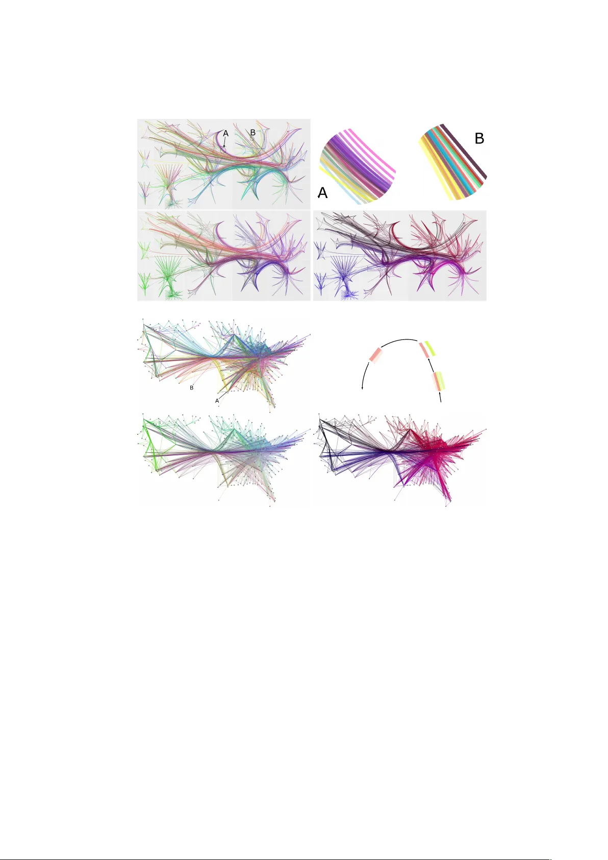
P eaco c k Bundles: Bundle Coloring for Graphs with Globalit y-Lo calit y T rade-off Jaakk o P eltonen 1 , 2 and Ziyuan Lin 1 1 Helsinki Institute for Information T ec hnology HI IT, Department of Computer Science, Aalto Universit y , Finland 2 Sc ho ol of Information Sciences, Univ ersity of T amp ere, Finland {jaakko.peltonen, ziyuan.lin}@aalto.fi Abstract. Bundling of graph edges (node-to-no de connections) is a common tec hnique to enhance visibility of o verall trends in the edge structure of a large graph lay out, and a large v ariety of bundling algo- rithms hav e been prop osed. How ev er, with strong bundling, it b ecomes hard to iden tify origins and destinations of individual edges. W e pro- p ose a solution: w e optimize edge coloring to differen tiate bundled edges. W e quantify strength of bundling in a flexible pairwise fashion betw een edges, and among bundled edges, we quantify ho w dissimilar their colors should b e b y dissimilarity of their origins and destinations. W e solve the resulting nonlinear optimization, which is also interpretable as a nov el dimensionalit y reduction task. In large graphs the necessary compro- mise is whether to differentiate colors sharply b etw een lo cally o ccurring strongly bundled edges (“local bundles”), or also b etw een the weakly bundled edges o ccurring globally o ver the graph (“global bundles”); we allo w a user-set global-lo cal tradeoff. W e call the technique “p eacock bun- dles”. Exp erimen ts show the coloring clearly enhances comprehensibility of graph lay outs with edge bundling. Keyw ords: Graph Visualization, Net work Data, Mac hine Learning, Di- mensionalit y Reduction. 1 In tro duction Graphs are a prominen t t yp e of data in visual analytics. Prominent graph types include for instance hyperlinks of webpages, so cial netw orks, citation net works b et w een publications, in teraction net works b et ween genes, v ariable dep endency net works of probabilistic graphical mo dels, message citations and replies in dis- cussion forums, traces of eye fixations, and many others. 2D or 3D visualization of graphs is a common need in data analysis systems. If node coordinates are not a v ailable from the data, sev eral no de la yout metho ds hav e b een developed, from constrained lay outs suc h as circular la youts ordered by no de degree to uncon- strained la youts optimized by v arious criteria; the latter metho ds can b e based on the no de and edge set (no de adjacency matrix) alone, or can mak e use of m ultiv ariate no de and edge features, typically aiming to reduce edge crossings and place no des close-b y if they are similar by some criterion. A B C D E F A B C D E F E d g e 1 E d g e 2 z 1 1 z 2 1 z 3 1 z 1 5 z 2 5 z 3 5 E d g e 3 z 1 3 Fig. 1: Illustration of p eaco c k bundle coloring. Left: A graph with no de groups A-F, dra wn with hierarc hical edge bund ling. With plain gray coloring finding the connecting v ertex pairs is not p ossible. Middle: P eacock bundle coloring reveals that nodes in group A connect to no des in group E in order, and similarly B to D in order, and C to F in reverse order. The connections are easily seen from the optimized coloring pro duced by our Peacock Bundles metho d: bundled edges tra veling from and to close-by no des get close-by colors. Righ t: P airwise bundling detection as describ ed in Section 3.1, for three edges, control p oin ts z ij sho wn as circles, distance threshold T as the radius of light gray circles (small threshold used for illustration). Con trol p oints z 12 , . . . , z 15 of edge 1 are near con trol points of edge 2, but only z 13 is near a con trol p oin t of edge 3. If, e.g., K ij = 2 nearby con trol p oin ts are required b et ween edges, edge 1 is considered bundled with edge 2 but not edge 3; edge 2 is considered bundled with edges 1 and 3, and edge 3 with edge 2 but not edge 1. Since edges 1 and 3 are not considered bundled they could b e assigned a similar color. In lay outs with numerous edges it may b e hard to see trends in no de-to-no de connections. Edge bundling dra ws multiple edges as curv es that are close-b y and parallel for at least part of their length. Bundling simplifies the app earance of the graph, and bundles also summarize connection trends b et w een areas of the la yout. How ev er, when edges are drawn close together, the ability to visually follo w edges and discov er their start and end p oin ts is lost. Interactiv e systems [10] can allo w insp ection of edges, but insp ecting numerous edges is lab orious. Comprehensibilit y of edges can be enhanced b y distinguishing them b y visual prop erties, such as line style, line width, markers along the curve, or color. F ollo wing an edge by its color can allo w an analyst to see where each edge go es, but po orly assigned colors can mak e this task hard to do at a glance. W e presen t a machine learning metho d that optimizes edge colors in graphs with edge bundling, to k eep bundled edges maximally distinguishable. W e fo cus on edge color as it has several degrees of freedom suitable for optimization (up to three con tinuous-v alued color channels if using R GB color space), but our metho d is easily applicable to other contin uous-v alued edge properties. W e call our solution p eaco c k bundles as it is inspired by the plumage of a p eacock; our metho d results in a fan of colors, reminiscen t of a peaco c k tail, at fan-in lo cations of edges arriving in to a bundle and fan-out lo cations of edges departing from a bundle. Figure 1 (middle) illustrates the concept and how it can help follow edges. W e next review related w orks and then presen t the metho d and experiments. 2 Bac kground: no de la yout, edge bundling, and coloring No de la youts of graphs hav e b een optimized by man y approaches, see [9] for a surv ey . Our approach is not specific to any node lay out approach and can be run for an y resulting lay out. Several metho ds hav e b een prop osed for edge bundling [4, 13, 6, 16, 7, 19, 17, 8]. F or example, Cui et al. [4] generate a mesh cov ering the graph on the displa y based on no de p ositions and edge distribution. The mesh helps cluster edges spatially; edges within a cluster are bundled. Hierarchical Edge Bundling [13] em b eds a tree representation for data with hierarc hy on to the 2D display . T ree no des are used as spline control p oints for edges; bundles come from reusing con trol p oin ts. See Zhou [22] for a recen t review and taxonom y . Unlik e no de lay out and edge bundling, relativ ely little attention has b een paid to practical edge coloring; while graph theory pap ers exist ab out the “edge coloring problem” of setting distinct colors to adjacent edges with a minimum n umber of colors, that combinatorial problem do es not reflect real-life graph visual analytics where a con tinuous edge color space exists and the task is to set colors to b e informativ e ab out graph prop erties. Simple coloring approaches exist. A naiv e coloring sets a random color to each edge: suc h coloring is unrelated to spatial positions of nodes and edges and is chaotic, making it hard to grasp an o verview of edge origins and destinations at a glance. Edge colors are sometimes reserv ed to show discrete or multiv ariate annotations such as edge strengths; suc h coloring relies on external data and ma y not help gain an ov erview of the graph lay out itself. A simple lay out-driven solution is to color each edge by onscreen p osition of the start or end no de. If edges ha ve b een clustered by some metho d, one often sets the same color to the whole cluster [7, 21]; this simplifies coloring, but preven ts telling apart origins and destinations of individual edges. Hu and Shi [15] create edge colorings with a maximal distinguishability moti- v ation related to ours, but their metho d do es not consider actual edge bundling and op erates on the original graph; w e op erate on bundled graphs and quantify edge bundling. Also, instead of only using binary detection of bundled edge pairs (a hard criterion whether t wo edges are bundled) we differentiate all edges, em- phasizing eac h pair b y a weigh t that is high betw een strongly bundled local edges and smaller betw een others, with a user-set global-lo cal tradeoff. Lastly , their metho d tries to set maximally distinct colors b et ween all bundled edges, needing harder compromises for larger bundles: w e quantify whic h bundled edges need the most distinct colors by comparing their origin and destination coordinates in the lay out, and thus can devote color resources efficiently ev en in large graphs. Our algorithm is related to nonlinear dimensionalit y reduction. Although dimensionalit y reduction has b een used in colorization for other domains [5, 3], to our knowledge ours is the first method to optimize lo cal graph coloring with edge bundling as a dimensionalit y reduction task. 3 The metho d: P eaco c k bundles Bundle coloring has several challenges. 1. Efficient coloring should dep end not only on high-dimensional graph prop erties on the low-dimensional graph lay out: if tw o edges are spatially distinct they do not need different colors. 2. Bun- d les ar e typic al ly not cle arly define d : the curve corresp onding to an individual edge may b ecome lo c al ly bundled with sev eral other edges at differen t places along the curve b et w een its start and end no de, and edges cannot be cleanly separated into groups that w ould corresp ond to some glob al ly nono v erlapping bundles. Solutions requiring nono verlapping bundles would b e sub optimal: they w ould either not b e applicable to real-life edge-bundled graphs or would need to artificially appro ximate the bundle structure of suc h graphs as nono verlapping subsets. 3. The solution should scale up to large graphs with large bundles. In large bundles it is t ypically not feasible to assign strongly distinct colors betw een all edges; it is then crucial to quantify how to make the compromise, that is, whic h edges should ha ve the most distinct colors within the bundle. Our coloring solution neatly solv es these challenges, by p osing the coloring as an optimization task defined based on lo cal bundling b et w een e ach individual p air of e dges . Our solution is applicable to all graphs and tak es in to account the full bundle structure in a graph la yout without approximations. F or any t wo edges it is easy to define whether their curves are bundled (close enough and parallel) for some part of their length, without requiring a notion of a globally defined bundle; w e optimize the coloring to tel l e ach e dge ap art fr om the ones it has b e en bund le d w ith . Such optimization makes maximally efficient use of the colors: tw o edges need distinct colors only if they are bundled together, whereas t wo edges that are not bundled can share the same color or v ery similar colors. Moreo ver, even b etw een tw o bundled edges, how distinct their colors need to b e can b e quan tified in a natural wa y based on the no de lay out: the more dissimilar their origins and destinations are, the more dissimilar their colors should b e. Differen tiating origins and destinations helps analysts assuming the no de lay out is meaningful. Computation of p eacock bundles requires tw o steps: 1. Dete ction of which p airs of e dges ar e bund le d to gether at some lo cation along their curv e. W e solv e this by a w ell-defined closeness threshold of consecutiv e curv e segmen ts. An edge ma y participate in m ultiple bundles along its curve. 2. Definition of the c olor optimization task . W e formalize the color assignmen t task as a dimensionalit y reduction task from t wo input matrices, a pairwise edge-to-edge bundling matrix and a dissimilarity matrix that quan tifies ho w dissimilar colors of bundled edges should b e, to a contin uous-v alued low- dimensional colorspace, which can be one-dimensional (1D) to ac hieve a color gradien t, or 2D or 3D for greater v ariety . (Prop erties like width or con tinuous line-st yle attributes could b e included in a higher than 3D output space; here w e use color only .) W e define the color assignment as an edge dissimilarity preserv ation task: colors are optimized to preserve spatial dissimilarities of start and end no des among eac h pair of bundled edges, whereas no constraint is placed b et w een colors of non-bundled edge pairs. P eaco c k bundle coloring can b e integrated into edge bundling algorithms, but can b e also run as standalone p ostprocessing for graphs with edge bundling, regardless of which algorithms yielded the no de lay out and edge curves. P eaco c k bundles optimize colors taking b oth the graph and its visualization (node and edge lay out) in to account: color separation needs to b e emphasized only for edges that appear spatially bundled. W e demonstrate the result on several graphs with differen t no de la youts and a p opular edge bundling technique. 3.1 Detection of bundled pairs of edges Let the graph con tain M edges i = 1 , . . . , M , each represented b y a curve. If the curves are spline curv es, let eac h curve be generated by C i con trol p oints; if the curves are piecewise linear, let each curv e b e divided into C i segmen ts represen ted e.g. b y the midp oin t of a segment. F or brevity w e use the terminology of control p oin ts in the following, but the algorithm can b e used just as well for other definitions of a curve, such as midp oin ts of piecewise linear curves or equidistributed p oin ts on the curv es if getting suc h lo cations is conv enient. Let B ij b e a v ariable in [0 , 1] denoting whether edge i is bundled together with edge j . If the edge bundling has b een created by an algorithm that explicitly defines bundle memberships for edges, B ij can simply b e set to 1 for edges assigned to the same bundle and zero otherwise. How ever, for sev eral situations this is insufficient: i) sometimes the bundling algorithm is not a v ailable or the bundling has e.g. b een created interactiv ely; ii) some bundling algorithms only e.g. attract edge segments and do not define which edges are bundled; iii) an edge may b e close to several differen t other edges, so that no single bundle mem b ership is sufficient to describ e its relationship to other edges. F or these reasons we provide a wa y to define pairwise edge bundling v ariables B ij that do es not require a v ailability of any previous bundling algorithm. W e set B ij = 1 if at least K ij consecutiv e control points of edge i are each close enough to one or more control p oints of edge j . In tuitively , if several con- secutiv e control p oin ts of edge i are close to edge j , the edges trav el close and parallel (as a bundle) at least b et ween those control p oints. Since our c hoice of con trol points do es not allow the curves to c hange drastically b et w een t wo con- secutiv e control points, the defined B ij is stable when the control point densities b et w een curve i and curv e j do not differ to o muc h. In practice, we set K ij to an in teger at least 1, separately for eac h pair of edges, as a fraction of the n umber of av ailable con trol points as detailed later in this section. F ormally , for edge i denote the on-screen co ordinates of the C i con trol p oints b y z i 1 , . . . , z iC i , and similarly for edge j . Let d ( · , · ) denote the Euclidean distance b et w een t wo control points, and let T b e a distance threshold. Then B ij = max r 0 =1 ,...,C i − K ij +1 r 0 + K ij − 1 Y r = r 0 1( min s =1 ,...,C j d ( z ir , z j s ) ≤ T ) (1) where r = r 0 , . . . , r 0 + K ij − 1 are indices of consecutive con trol p oin ts in edge i . The term 1( · ) is 1 if the statement inside is true and zero otherwise: that is, the term is 1 if the r th control p oin t of edge i is close to edge j (to some con trol p oin t s of edge j ). The whole pro duct term is 1 if the K ij consecutiv e control p oin ts of i from r 0 on wards are all close to edge j . Finally , the whole term B ij is 1 if edge i has K ij consecutiv e p oin ts (from any r 0 on wards) that are all close to edge j . Figure 1 (righ t) illustrates the pairwise bundling detection. The distance threshold T should b e set to a v alue b elo w which line segmen ts app ear very similar; a rule of thum b is to set T to a fraction of the total diameter (or larger dimension) of the screen area of the graph. Similarly , a con venien t w ay to set the required num ber of close-by control p oin ts K ij is to set it to a fraction of the maxim um num b er of control points in the tw o edges, requiring at least 1 control p oin t, so that for eac h pair of edges i and j we set K ij = max(1 , b max( C i , C j ) K min c ) where K min ∈ (0 , 1] is the desired fraction. Detected pairwise bundles match ground truth in all simple examples we tried (e.g. Fig. 1 left); in exp erimen ts of Section 4 where no ground truth is av ailable the bundling is visually go od; edges bundled with any edge of in terest can be in teractively chec k ed at http://ziyuang.github.io/peacock- examples/ . 3.2 Optimization of edge colors by dimensionality reduction Our coloring is based on dimensionality reduction of bundled edges from an original dissimilarity (distance) matrix to a color space; we thus need to define ho w dissimilar tw o bundled edges are. W e aim to help analysts differen tiate where in the graph lay out eac h edge go es; we thus use the no de lo cations of edges to define the similarity . Denote the tw o on-screen no de lay out co ordinates of edge i by v 1 i and v 2 i . W e first define d original ij = min( k v 1 i − v 1 j k + k v 2 i − v 2 j k , k v 1 i − v 2 j k + k v 2 i − v 1 j k ) . (2) Denote the set of p features for edge i as a v ector x i = [ x i 1 , . . . , x ip ], and denote the low-dimensional output features for edge i as a vector y i = [ y i 1 , . . . , y iq ] where q ∈ { 1 , 2 , 3 } is the output dimensionalit y . W e define the dimensionality reduction task as minimizing the difference b et w een the endp oint dissimilarity of bundled edges and dissimilarity of their optimized colors. This yields the cost function min { y 1 ,..., y M } X i X j B ij ( d orig inal ij − d out ( y i , y j )) 2 (3) where d out ( y i , y j ) is the Euclidean distance b et ween the output features. The terms B ij are large for only those pairs of edges that are bundled, thus minimiz- ing the cost assigns colors to preserve dissimilarit y within bundled edges, but allo ws freedom of color assignment b et w een non-bundled edges. The cost en- capsulates that greater difference of edge destinations should yield greater color difference, and that color differen tiation is most needed for strongly bundled edges. While alternative formulations are p ossible, (3) is simple and works well. F rom lo cal to global color differen tiation. The w eights B ij detect edges according to thresholds T and K ij . Some edge pairs that fail the detection migh t still visually app ear nearly bundled: instead of differentiating only within de- tected bundles, it is meaningful to differen tiate other edges to o. The simplest w ay is to enco de a tr ade off b etw een lo cal (within-bundle) and global differenti- ation in the B ij : we set B ij = 1 if edges i and j are bundled, otherwise B ij =  where  ∈ [0 , 1] is a user-set parameter for the preferred global-lo cal tradeoff. When 0 <  < 1, the cost emphasizes achieving desired color differences b e- t ween bundled edges (where B ij = 1) according to their dissimilarity of origins and destinations, but also aims to ac hieve color differences b et ween other edges ( B ij =  ) according to the same dissimilarity . As the optimization is based on desired dissimilarities b et ween edges, it in telligently optimizes colors ev en when all edge pairs can hav e nonzero weigh t:  = 0 means a pure local coloring where only bundled edge pairs matter, and  = 1 means a pure global coloring that aims to show dissimilarity of origin and destination for all edges regardless of bundling. In our tests coloring c hanges gradually with resp ect to  . In exp eri- men ts, when emphasizing local color differences, w e set  = 0 . 001 whic h achiev ed lo cal differen tiation and formed color gradients for bundles in most cases. A wa y to set a more nuanced tradeoff is to run edge detection with multiple settings and set w eaker B ij for edges detected with weak er thresholds; in practice the ab o ve simple tradeoff already w orked w ell. Relationship to nonlinear multidimensional scaling. Interestingly , min- imizing (3) can b e seen as a sp ecialized weigh ted form of nonline ar multidimen- sional sc aling , with sev eral differences : unlike traditional multidimensional scal- ing we treat edges (not data items or no des) as input items whose dissimilarities are preserved; our output is not a spatial lay out but a color sc heme; and most im- p ortan tly , the cost function do es not aim to preserv e all “distances” but weigh ts eac h pairwise distance according to ho w strongly that pair of edges is bundled. The theoretical connection lets us mak e use of optimization approac hes previ- ously developed for multidimensional scaling, here w e choose to use the p opular stress ma jorization algorithm (SMACOF) [1] to minimize the cost function. Color range normalization. After optimization, output features y i of eac h edge must b e normalized to the range of the color c hannels (or p ositions along a color gradient). Simple ideas like applying an affine transform to the output matrix Y = ( y 1 , . . . , y M ) w ould give different amoun ts of color space to differen t bundles, th us colors within bundles would not be well differentiated. W e prop ose a normalization to maximally distinguish edges within each bundle. Let C ol denote the color matrix to b e obtained from normalization. F or each y i , let { y i l } M i l =1 b e the set of output features where each edge l is bundled with edge i . W e assemble y i and { y i l } M i l =1 in to a matrix Y i = ( y i , y i 1 , . . . , y i M i ), affinely transform Y i to ˜ Y i = ( ˜ y i , ˜ y i 1 , . . . , ˜ y i M i ) so that eac h entry in ˜ Y i is within the allo wed range (say , [0 , 1]), then set C ol i , the i -th column of C ol (color vector for edge i ) as ˜ y i . This normalization expands the color range within bundles. Where to sho w colors. The optimized colors can b e sho wn along the whole edge, or at “fan-in” segmen ts where the edge en ters a bundle and “fan- out” segments where it departs a bundle. Edge i is bundled with j if sev eral consecutiv e curv e segmen ts of i are close to j ; the last segment b efore the close-b y ones is the fan-in segment; the first segmen t after the close-by ones is the fan-out segmen t. In exp eriments w e show color along the whole edge for simplicity . Note that, as with any edge coloring, colors of close-b y edges may perceptually blend, but our optimized colors then remain visible at fan-in and fan-out lo cations. Fig. 2: Colorings for the graph “radial”. T op left : the coloring from P eaco c k with  = 0 . 001. T op right : zo omed-in versions of the parts within dashed-line circles in the top-left figure as examples of lo cal coloring. In the four zoomed-in parts, colors show a linear gradient and v ary in yello w-red-blue, th us 1) lo cal colors are differen tiated, and 2) they span roughly the same full color range. The lo cal colors also help follo w edges at b ottom right of the graph, where colors are ho- mogeneous in the baseline coloring. Bottom left : coloring from Peacock,  = 1. The bundles are colored in to 3 parts: the blue-ish upp er half, green-ish low er-left part, and yello w-ish low er-righ t part. There are also red bundles joining the blue and green parts, differen tiating itself from other bundles. Bottom righ t : the baseline coloring. The bundles are colored into the red-ish upp er half and blue- ish low er half. C ompared with the coloring with  = 1 from Peacock, the bundle from left to righ t, and the bundle at the top-left corner are less distinguishable. 4 Exp erimen ts W e demonstrate the P eaco c k bundles metho d on five graphs (Figs. 2–4): tw o graphs with hierarchical edge bundling [13], and three with force-directed edge bundling [14]. The t wo graphs with hierarchical edge bundling are created from the class hierarc hy of the visualization to olkit Flare [11], with the built-in radial la yout (graph named “radial”; Fig. 2) and tree map lay out (“tree map”; Fig. 3a) in d3.js [2] resp ectiv ely . The four graphs with force-directed edge bundling are: a spatial graph of US fligh t connections (“airline”; Fig. 3b); a graph of consecutiv e w ord-to-word appearances in no v els of Jane Austen (“Jane Austen”; Fig. 4); and a graph of matches betw een US college football teams (“fo otball”; Fig. 5). The last three graphs are laid out as an unconstrained 2D graph by a recent no de- neigh b orho od preserving lay out method [18]. F or all graphs, edge bundles were created b y a d3.js plugin implementing the algorithm [20] adapted to splines. All coloring are compared with a baseline coloring from end p oin t p ositions. The baseline . W e compare our metho d with a baseline coloring that directly enco des end p oin t p ositions into color channels. W e choose c hannel red and blue for the enco ding in the exp erimen ts. Let v 1 i = ( x 1 i , y 1 i ) and v 2 i = ( x 2 i , y 2 i ) be the onscreen co ordinates of edge i ’s tw o end p oin ts as in (2). W e first create a 3-dimensional vector g C ol baseline i as the “unnormalized” color for edge i as g C ol baseline i = (min( x i, 1 , x i, 2 ) , 0 , min( y i, 1 , y i, 2 )) T (4) then w e affinely normalize the matrix g C ol baseline in to [0 , 1] to obtain the final baseline colors C ol baseline . Choices of P eaco c k parameters . The parameters T and K min in (1) m ust b e c hosen to determine B ij . W e set T to 2% ∼ 4% of max(graph width , graph height), and fix K min as 0.4. Exp erimen ts show the choices giv e go od results empirically . Figures 2 – 4 sho w the results from the prop osed metho d and the baseline. The top-left subfigures are with the tradeoff parameter set to prefer lo calit y in the coloring. The top-righ t subfigures provide zo omed-in views detailing the local color v ariation (“p eaco c k fans”) and demonstrating how the coloring improv es readabilit y and helps follow edges. The b ottom-left figures are optimized to dif- feren tiate origins and destinations globally (tradeoff parameter  = 1), hence colors indicate o verall trends of connections betw een areas of the graph lay out, at the expense of less color v ariabilit y within bundles. The bottom-right figures are from the baseline, also aiming to sho w v ariability of endpoint p ositions the coloring but not optimized by machine learning; the simple baseline coloring lea ves bundles and within-bundle v ariation less distinguishable. 5 Conclusions W e introduced “p eaco c k bundles”, a no vel edge coloring algorithm for graphs with edge bundling. Colors are optimized b oth to preserve differences b et w een bundle lo cations, and differentiate edges within bundles. The algorithm is based on dimensionality reduction without need to explicitly define bundles. Exp eri- men ts sho w the metho d outp erforms the baseline coloring with several graphs and bundling algorithms, greatly impro ving the comprehensibilit y of graphs with edge bundling. Poten tial future work includes incorp orating color p erception mo dels [12], and more nuanced weigh ting schemes for global-lo cal tradeoffs. W e ac knowledge computational resources from the Aalto Science-IT pro ject. Authors b elong to the COIN centre of excellence. The w ork was supp orted by Academ y of Finland gran ts 252845 and 256233. A (a) Different coloring for “tree map” A B (b) Different coloring for “airline” Fig. 3: Colorings for the graphs “tree map” and “airline”. In b oth subfigures: top left : the colorings from Peacock with  = 0 . 001. In Fig. 3a, the lo cal linear gradien t is clearer at the the ends of the bundles. I n Fig. 3b, the large bundle in the middle shows the lo cal coloring, by separating the bundle in to the upp er blue dominating part, the middle red-ish part, and the low er lighter part. T op righ t : examples of ho w the colorings enhance readabilit y by inv estigating the parts within dashed line circles in b oth top-left subfigures. In Fig. 3a, the colors in bundle A help the user to recognize, for example, 1) the blue-ish part in bundle A leads to the blue-ish part of the top-right “claw” or the right “claw”; 2) the red-ish part in bundle A leads to the red-ish part of the “claw” at the right of bundle B, or the top right “cla w”; 3) the yello w-ish half that joins in the middle leads to bundle B or to the “claw” at the righ t of bundle B. Fig. 3b shows how the coloring help a pink edge from A to B stand out against other edges in the same bundle. Bottom left : the coloring from Peacock with  = 1. In Fig. 3a, bundles are globally differentiated. In Fig. 3b, for no des of large degrees, the edges connecting to them hav e distinct colors for different directions. Bottom righ t : the baseline coloring. In Fig. 3a, the user ma y mis-recognize that there are edges from bundle A to bundle B. In Fig. 3b, unlike the b ottom-left subfigure, edges connecting to the same no de tend to hav e similar colors. Fig. 4: Colorings for graph “Jane Austen”. T op left : the coloring from P eaco c k with  = 0 . 001. The “crossing” at the right half of the figure sho ws a clear differen tiation: red edges go from upp er-righ t to lo wer-left; green edges go from upp er to lo wer; blue edges go from upp er-left to low er-righ t. Without the lo cal coloring, it is difficulty to tell whether the bundles or the edges are crossing or just tangental to one another. T op right : another example from the zoomed-in v ersion of the part within the dashed line circle in the top-left figure. Edge colors c hange from green to purple-ish. The colors help the user follow the edges after the heavily bundled part in the middle: red edges mostly go leftw ards, green edges are scattered, and blue edges mostly go right w ards. Bottom left : the coloring from P eaco c k with  = 1. Less lo calit y but more globality . The earlier blue edges in the right “crossing” b ecome purple, but still distinguishable from the other tw o bundles. Bottom right : the baseline coloring, whic h loses the distinguishablit y sho wn in the P eaco c k coloring. A B Fig. 5: Colorings for graph “football”. textbfT op left: the coloring from Peacock with  = 0 . 001. The uncertain t y in this graph is mostly from the small clusters of no des at the end of the edges. T op right : an example showing how the coloring help distinguish heavily bundled edges from A to B. The sho wn segmen ts are the zo omed-in version of the parts within the dashed line circle or ellipse in the top-left figure. W e can see, for example, that the blue edge leads to the top no de in B, while the yello w edge leads to leftmost no de in B. This is also noticeable in the top-left figure, particularly for the blue edge. How ev er, it will b e a difficult task with the baseline coloring since the the part betw een A and B is hea vily bundled. Bottom left : the coloring from Peacock with  = 1. Colors of edges from the same cluster are differentiated (e.g., at the top-left cluster, edge colors v ary from red to blue). Bottom righ t : the baseline coloring, which only reflects the lo cations of the bundles. References 1. Borg, I., Gro enen, P .J.F.: Mo dern Multidimensional Scaling: Theory and Applica- tions (Springer Series in Statistics). Springer, 2 edn. (Aug 2005) 2. Bosto c k, M., Ogiev etsky , V., Heer, J.: D3 data-driven do cumen ts. IEEE T. Vis. Comput. Gr. 17(12), 2301–2309 (2011) 3. Casaca, W allace et al.: Colorization b y multidimensional pro jection. In: Proc. SIB- GRAPI 2012. pp. 32–38. IEEE (2012) 4. Cui, W., Zhou, H., Qu, H., W ong, P .C., Li, X.: Geometry-based edge clustering for graph visualization. IEEE T. Vis. Comput. Gr. 14(6), 1277–1284 (2008) 5. Daniels, J., Anderson, E.W., Nonato, L.G., Silv a, C.T., et al.: In teractive vector field feature identification. IEEE T. Vis. Comput. Gr. 16(6), 1560–1568 (2010) 6. Dwy er, T., Marriott, K., Wybrow, M.: Integ rating edge routing into force-directed la yout. In: Kaufmann, M., W agner, D. (eds.) Pro c. GD 2006. pp. 8–19. Springer (2006) 7. Erso y , O., Hurter, C., P aulovic h, F.V., Can taneira, G., T elea, A.: Skeleton-based edge bundling for graph visualization. IEEE T. Vis. Comput. Gr. 17(12) (2011) 8. Gansner, E.R., Hu, Y., North, S., Scheidegger, C.: Multilevel agglomerativ e edge bundling for visualizing large graphs. In: Pro c. PacificVis 2011. pp. 187–194. IEEE (2011) 9. Gibson, H., F aith, J., Vick ers, P .: A surv ey of tw o-dimensional graph la yout tech- niques for information visualisation. Info. Vis. 12(3-4), 324–357 (2013) 10. Grossman, T., Balakrishnan, R.: The bubble cursor: enhancing target acquisition b y dynamic resizing of the cursor’s activ ation area. In: Pro c. CHI 2005. pp. 281– 290. ACM (2005) 11. Heer, J.: Flare. https://git.io/v6buH (2009) 12. Heer, J., Stone, M.: Color naming models for color selection, image editing and palette design. In: Pro c. CHI 2012 (2012) 13. Holten, D.: Hierarchical edge bundles: Visualization of adjacency relations in hier- arc hical data. IEEE T. Vis. Comput. Gr. 12(5), 741–748 (2006) 14. Holten, D., V an Wijk, J.J.: F orce-directed edge bundling for graph visualization. Comput. Graph. F orum 28(3), 983–990 (2009) 15. Hu, Y., Shi, L.: A coloring algorithm for disambiguating graph and map drawings. In: Duncan, C., Symv onis, A. (eds.) Pro c. GD 2014. pp. 89–100. Springer (2014) 16. Hurter, C., Erso y , O., T elea, A.: Graph bundling by k ernel densit y estimation. Comput. Graph. F orum 31(3pt1), 865–874 (2012) 17. Luo, S.J., Liu, C.L., Chen, B.Y., Ma, K.L.: Ambiguit y-free edge-bundling for in- teractiv e graph visualization. IEEE T. Vis. Comput. Gr. 18(5), 810–821 (2012) 18. P arkkinen, J., Nyb o, K., Peltonen, J., Kaski, S.: Graph visualization with latent v ariable mo dels. In: Pro c. MLG 2010. pp. 94–101. ACM (2010) 19. Pup yrev, S., Nachmanson, L., Kaufmann, M.: Improving la yered graph lay outs with edge bundling. In: Brandes, U., Cornelsen, S. (eds.) Pro c. GD 2010. pp. 329– 340. Springer (2010) 20. Sugar, C.: d3.forcebundle. https://git.io/v6GgL (2016) 21. T elea, A., Erso y , O.: Image-based edge bundles: Simplified visualization of large graphs. Comput. Gr. F orum 29(3), 843–852 (2010) 22. Zhou, H., Xu, P ., Y uan, X., Qu, H.: Edge bundling in information visualization. Tsingh ua Science and T echnology 18(2), 145–156 (2013)