Convolutional Neural Networks for Text Categorization: Shallow Word-level vs. Deep Character-level

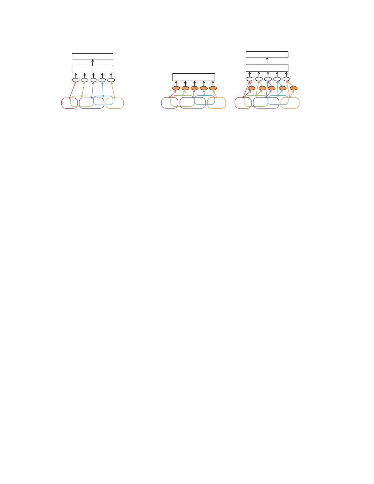
Con v olutional Neural Networks for T e xt Categorization: Shallo w W ord-le vel vs. Deep Character -le v el Rie Johnson RJ Research Consulting, NY , USA riejohnson@gmail.com T ong Zhang Rutgers Uni versity , NJ, USA tzhang@stat.rutgers.edu Abstract This paper reports the performances of shallow w ord-lev el con volutional neural networks (CNN), our earlier w ork (2015) [3, 4], on the eight datasets with relativ ely large training data that were used for testing the very deep character- lev el CNN in Conneau et al. (2016) [1]. Our findings are as follows. The shallow word-lev el CNNs achieve better error rates than the error rates reported in [1] though the results should be interpreted with some consideration due to the unique pre-processing of [1]. The shallo w word-lev el CNN uses more parameters and therefore requires more storage than the deep character-le vel CNN; ho we ver , the shallow word-le vel CNN computes much faster . 1 Intr oduction T ext categorization is the task of labeling documents, which has many important applications such as sentiment anal- ysis and topic categorization. Recently , sev eral v ariations of con volutional neural networks (CNNs) [7] ha ve been shown to achiev e high accurac y on te xt categorization (see e.g., [3, 4, 9, 1] and references therein) in comparison with a number of methods including linear methods, which had long been the state of the art. Long-Short T erm Memory networks (LSTMs) [2] hav e also been shown to perform well on this task, riv aling or sometimes exceeding CNNs [5, 8]. Ho wev er , CNNs are particularly attracti ve since, due to their simplicity and parallel processing-friendly nature, training and testing of CNNs can be made much faster than LSTM to achiev e similar accurac y [5], and therefore CNNs hav e a potential to scale better to large training data. Here we focus on two CNN studies that report high performances on categorizing long documents (as opposed to cate gorizing individual sentences): • Our earlier work (2015) [3, 4]: shallow wor d-level CNNs (taking sequences of words as input), which we abbreviate as wor d-CNN . • Conneau et al. (2016) [1]: very deep character -level CNNs (taking sequences of characters as input), which we abbreviate as c har -CNN . Although both studies report higher accuracy than pre vious work on their respecti ve datasets, it is not clear how they compare with each other due to lack of direct comparison. In [1], the v ery deep char -CNN was shown to perform well with larger training data (up to 2.6M documents) but perform relativ ely poorly with smaller training data; e.g., it underperformed linear methods when trained with 120K documents. In [3, 4] the shallow word-CNN was shown to perform well, using training sets (most intensively , 25K documents) that are mostly smaller than those used in [1]. While these results imply that the shallow word-CNN is likely to outperform the deep char-CNN when trained with relativ ely small training sets such as those used in [3, 4], the shallow word-CNN is untested on the training sets as large as those used in [1]. Hence, the purpose of this report is to fill the gap by testing the shallow word-CNNs as in [3, 4] on the datasets used in [1], for direct comparison with the results of very deep char -CNNs reported in [1]. Limitation of work In this work, our new experiments are limited to the shallow word-CNN as in [3, 4]. W e do not provide new error rate results for the very deep CNNs proposed by [1], and we only cite their results. Although it may be natural to assume that the error rates reported in [1] well represent the best performance that the deep char-CNNs 1 can achie ve, we note that in [1], documents were clipped and padded so that they all became 1014 characters long, and we do not know how this pre-processing affected their model accuracy . T o experiment with word-CNN, we handle variable-sized documents as variable-sized as we see no merit in making them fixed-sized, though we reduce the size of v ocabulary to reduce storage requirements. Considering that, we emphasize that this work is not intended to be a rigorous comparison of word-CNNs and char-CNNs; instead, it should be regarded as a report on the shallow word- CNN performance on the eight datasets used in [1], referring to the results in [1] as the state-of-the-art performances. 1.1 Preliminary W e start with briefly revie wing the very deep word-CNN of [1] and the shallo w word-CNN of [3, 4]. 1.1.1 V ery deep character-le vel CNNs of [1] [1] proposed very deep char-CNNs and sho wed that their best performing models produced higher accurac y than their shallower models and pre vious deep char-CNNs of [9]. Their best architecture consisted of the following: • Character embedding of 16 dimensions. • 29 con v olution layers with the number of feature maps being 64, 128, 256, and 512. • T wo fully-connected layers with 2048 hidden units each, following the 29 con volution layers. • One of the following three methods for downsampling to halve the temporal size: setting stride to 2 in the con v olution layer , k -max pooling, or max-pooling with stride 2. Downsampling was done whene ver the number of feature maps was doubled. • k -max pooling with k =8 to produce 4096-dimensional input (per document) to the fully-connected layer . • Batch normalization. The kernel size (‘region size’ in our w ording) was set to 3 in e very con volution layer . In addition, the results obtained by two more shallo wer architectures were reported. [1] should be consulted for the exact architectures. 1.1.2 Shallow word-level CNNs as in [3, 4] T wo types of w ord-CNN were proposed in [3, 4], which are illustrated in Figure 1. One is a straightforw ard application of CNN to text (the base model), and the other in volv es training of tv-embedding (‘tv’ stands for two views) to produce additional input to the base model. The models with tv-embedding produce higher accuracy pro vided that suf ficiently large amounts of unlabeled data for tv-embedding learning are available. As discussed in [5], the shallow word-CNN can be regarded as a special case of a general framework which jointly trains a linear model with a non-linear feature generator consisting of ‘text re gion embedding + pooling’, where text r e gion embedding is a loose term for a function that con verts re gions of text (word sequences such as “good buy”) to vectors while preserving information relev ant to the task of interest. W ord-CNNs without tv-embedding (base model) In the simplest configuration of the shallow word-CNNs, the region embedding is in the form of f ( x ) = σ ( Wx + b ) where σ is a component-wise nonlinear function (typically σ ( x ) = max( x, 0) ), input x represents a text region via either the concatenation of one-hot vectors for the words in the region or the bow representation of the region, and weight matrix W and bias vector b (shared within a layer) are trained. Note that when x is the concatenation of one- hot v ectors, Wx can be interpreted as summing position-sensitive word vectors, and when x is the bo w representation of the region, Wx can be interpreted as summing position-insensitive word vectors. Thus, in a sense, the region embedding f ( x ) abov e internally and implicitly includes word embedding, as opposed to having an external and 2 A good buy ! Pooling Linear classifier (a) w ord-CNN (base model). A good buy ! Linear classifier Step 1. T rain tv-embedding with two-view embedding learning objectives. Step 2. T r a i n w / t a r ge t l a b e l s . A good buy ! Pooling Linear classifier S t e p 2. T rain w/ target labels. (b) w ord-CNN with tv-embedding. Figure 1: Shallow word-lev el CNNs. In each oval, computation in the form of σ ( Wx + b ) takes place, where x is input, parameters W and b (shared within a layer) are trained, and σ is component-wise nonlinearity , typically σ ( x ) = max(0 , x ) . In the base model in (a), input x is one-hot representation of each text region (e.g., “good buy”). In (b) we first train tv-embedding with two-vie w embedding learning objectiv es and then use it to produce additional input to the base model. explicit word embedding layer before a con v olution layer as in, e.g., [6], which makes x the concatenation of word vectors. See also the supplementary material of [4] for the representation po wer analysis. As illustrated in Figure 1 (a), f ( x ) is applied to the text regions at every location of a document (ov als in the figure), and pooling aggregates the resulting region vectors into a document vector , which is used as features by a linear classifier . In our experiments with word-CNN without tv-embedding reported below , the one-hot representation used for x was fixed to the concatenation of one-hot vectors with a vocab ulary of the 30K most frequent words, and the dimensionality of region embedding (i.e., the number of feature maps) was fixed to 500. That is, our one-hot vectors were 30K-dimensional while any out-of-v ocabulary word was con verted to a zero vector , and the region embedding f ( x ) produced 500-dimensional vectors for each region. Region size (the number of words in each region) was chosen from { 3,5 } . Based on our previous work, we performed max-pooling with k pooling units (each of which covers 1 /k of a document) while setting k = 1 on sentiment analysis datasets and choosing k from { 1 , 10 } on the others. The models described here also served as the base models of the word-CNN with tv-embedding described ne xt. W ord-CNNs with tv-embedding Training of word-CNNs with tv-embedding is done in two steps, as sho wn in Figure 1 (b) . First we train region tv-embedding (‘tv’ stands for two views) in the form of f ( x ) above, with a two-vie w embedding learning objecti ve such as ‘predict adjacent text regions (one view) based on a text region (the other view)’. This training can be done with unlabeled data. [4] provides the definition and theoretical analysis of tv-embeddings. Next, we use the tv-embedding to produce additional input to the base model and train it with labeled data. This model can be easily extended to use multiple tv-embeddings, each of which, for example, uses a distinct vector representation of re gion, and so the region embedding function in the final model (hollow ov als in Figure 1 (b)) can be written as: g ( x , { x ( i ) } i ) = σ Wx + X i W ( i ) x ( i ) + b ! . x ( i ) is the output of the tv-embedding index ed by i applied to the corresponding text region. In [4], tv-embedding training was done using unlabeled data as an additional resource; therefore, the proposed models were semi-supervised models. In the experiments reported below , due to the lack of standard unlabeled data for the tested datasets, we trained tv-embeddings on the labeled training data ignoring the labels; thus, the resulting models are supervised ones. W e trained four tv-embeddings with four distinct one-hot representations of text regions (i.e., input to orange ovals in Figure 1 (b)): bow representation with region size 5 or 9, and bag-of- { 1,2,3 } -gram representation with region size 5 or 9. T o make bo w representation for tv-embedding, we used a vocab ulary of the 30K most frequent words, and to make the bag-of- { 1,2,3 } -gram representation, we used a vocab ulary of the 200K most frequent { 1,2,3 } -grams. The 3 dimensionality of tv-embeddings was 300 unless specified otherwise, and the dimensionality of g ( · ) w as 500 (as in the base model); thus, we note that the dimensionality of internal vectors are comparable to those of the deep char -CNN of [1], which are 64, 128, 256, and 512 as sho wn belo w . The rest of the setting was the same as the base model abov e. Other two-step approaches Another two-step approach with word-CNNs was studied by [6], where the first step is pre-training of the word embedding layer (substituted by use of public word vectors in [6]), which is followed by a con v olution layer . One potential advantage of our tv-embedding learning is that it can learn more complex information (embedding of wor d sequences ) than w ord embedding (embedding of single wor ds in isolation ). 2 Experiments W e report the experimental results of the shallow word-CNNs in comparison with the results reported in [1]. The experiments can be reproduced using the code a v ailable at riejohnson.com/cnn_download.html . 2.1 Data and data prepr ocessing The eight datasets used in [1] are summarized in T able 1 (a). A G and Sogou are news, Dbpedia is an ontology , and Y elp and Amazon (abbreviated as ‘ Ama’) are revie ws. ‘.p’ (polarity) in the names of revie w datasets indicates that labels are either positive or ne gati ve, and ‘.f ’ (full) indicates that labels represent the number of stars. Y ahoo contains questions and answers from the ‘Y ahoo! Answers’ website. On all datasets, classes are balanced. Sogou consists of Romanized Chinese. The others are in English though some contain characters of other languages (e.g., Chinese, K orean) in small proportions. T o experiment with the deep char -CNNs, [1] con verted upper-case letters to lower -case letters and used 72 charac- ters (lower -case alphabets, digits, special characters, and special tok ens for padding and out-of-vocab ulary characters). They padded the input text with a special token to a fixed size of 1014. T o experiment with the shallow word-CNNs, we also con verted upper-case letters to lower-case letters. Unlike [1], we handled variable-sized documents as variable-sized without any shortening or padding; howe ver , we limited the vocab ulary size to 30K words and 200K { 1,2,3 } -grams, as described above. T o put it into perspective, the size of the complete word vocabulary of the largest training set (Ama.p) is 1.3M, and when limited to the words with frequency no less than 5, it is 221K. By comparison, a vocab ulary of 30K sounds rather small, but it co vers about 98% of the te xt on Ama.p, and it appears to be sufficient for obtaining good accurac y . 2.2 Experimental details of word-lev el CNNs On all datasets, we held out 10K data points from the training set for use as validation data. Models were trained using the training set minus v alidation data, and model selection (or hyper parameter tuning) was done based on the performance on the validation data. Tv-embedding training was done as in [4]; weighted square loss was minimized without regularization while the target regions (adjacent regions) were represented by bo w vectors, and the data weights were set so that the negati ve sampling effect was achieved. Tv-embeddings were fixed (i.e., no weight updating) during the final training with labeled data. T raining with labels (either with or without tv-embedding) w as done as follo ws. A log loss (or cross entrop y) with softmax was minimized. Optimization was done by mini-batch SGD with momentum 0.9 and the mini-batch size was set to 100. The number of epochs was fixed to 30 (except for A G, the smallest, for which it was fixed to 100), and the learning rate was reduced once by multiplying 0.1 after 24 epochs (or 80 epochs on A G). In all layers, weights were initialized by the Gaussian distribution of zero mean and standard de viation 0.01. The initial learning rate was treated as a hyper parameter . Regularization was done by applying dropout with 0.5 to the input to the top layer and having a L2 regularization term with parameter 0.0001 on the top layer weights. 4 (a) Data statistics A G Sogou Dbpedia Y elp.p Y elp.f Y ahoo Ama.f Ama.p # of training documents 120K 450K 560K 560K 650K 1.4M 3M 3.6M # of test documents 7.6K 60K 70K 38K 50K 60K 650K 400K # of classes 4 5 14 2 5 10 5 2 A verage length (words) 45 578 55 153 155 112 93 91 A verage length (characters) 219 2709 298 710 718 519 441 432 (b) Error rates (%) Models depth A G Sogou Dbpedia Y elp.p Y elp.f Y ahoo Ama.f Ama.p Linear model best [9] 0 7.64 2.81 1.31 4.36 40.14 28.96 44.74 7.98 char-CNN best [1] 9+2 9.17 3.58 1.35 4.88 36.73 27.60 37.95 4.70 29+2 8.67 3.18 1.29 4.28 35.28 26.57 37.00 4.28 word-CNN w/o tv-embed. 1 6.95 2.21 1.12 3.44 34.21 26.06 37.51 4.27 word-CNN w/ tv (300-dim) 2 6.57 1.89 0.84 2.90 32.39 24.85 36.24 3.79 T able 1: (a) Data statistics. (b) Error rates (%). ‘depth’ counts the hidden layers with weights in the longest path. [9] reported the results of several linear methods, and we copied only the best results. [1] reported the results of deep char-CNN with three downsampling methods, and we copied only the best results. The word-CNN results are our ne w results. The best (or second best) results are shown in bold (or italic) font, respecti vely . 2.3 Perf ormance results Error rates In T able 1 (b), we show the error rate results of the shallow word-CNN in comparison with the best results of the deep char-CNN reported in [1] and the best results of linear models reported in [9]. On each dataset, the best results are shown in bold and the second best results are sho wn in the italic font. On all datasets, the shallow word-CNN with tv-embeddings performs the best. The second best performer is the shallow word-CNN without tv-embedding on all but Ama.f (Amazon full). Whereas the deep char-CNN under- performs traditional linear models when training data is relatively small, the shallow word-CNNs with and without tv-embedding clearly outperform them on all the datasets. W e observe that, as in our previous work [4], additional input produced by tv-embeddings led to substantial improv ements. The performances of word-CNN without tv-embedding might be further improv ed by having multiple region sizes [3, 6], but for simplicity , we did not attempt it in this work. Model size and computation time In T able 2, we observe that, compared with the deep char -CNN, the shallow wor d-CNN has mor e parameters but computes much faster . Although the table shows computation time and error rates on one particular dataset (Y elp.f), the observation was the same on the other datasets. The shallow word-CNN has more parameters because the number of parameters mostly depends on the vocabulary size, which is large with word-CNN (30K and 200K in our e xperiments) and small with char -CNN (72 in [1]). Nevertheless, computation of the shallow word-CNN can be made much faster than the deep char -CNN for three reasons 1 . First, with implementation to handle sparse data efficiently , computation of shallow word-CNN does not depend on the vocabulary size. For example, when x is the concatenation of p one-hot vectors of dimensionality v (vocab ulary size), computation time of Wx (the most time-consuming step) depends not on v (e.g., 30K) but on p (e.g., 3) since we only need to multiply nonzero elements of x with the weights in W . Second, character-based methods need to process about fiv e times more text units than w ord-based methods; compare the ro ws of av erage length in words and characters in T able 1 (b). Third, a deeper network is less parallel processing-friendly since many layers ha ve to be processed sequentially . If we reduce the dimensionality of tv-embedding from 300 to 100, the number of parameters can be reduced to a half with a small de gradation of accurac y , as sho wn in T able 2; more error rate results with 100-dim tv-embedding are 1 Computation time depends on the specifics of both implementation and en vironment including hardware. Our discussion here assumes parallel processing and efficient handling of sparse matrices (whose components are mostly zero), and otherwise it is general. 5 Depth Dimensionality of #param T ime Error layer outputs (#layers) rate(%) char-CNN [1] 9+2 16(1), 64(3), 128(2), 2.2M † 215 36.73 256(2), 512(2), 2048(2) 29+2 16(1), 64(11), 128(10), 4.6M ‡ 700 35.28 256(4), 512(4), 2048(2) word-CNN w/o tv-embed. 1 500(1) 45M 6 34.21 w/ 2 tv (100-dim) 2 100(2), 500(1) 68M 21 32.77 w/ 4 tv (100-dim) 2 100(4), 500(1) 91M 36 32.55 w/ 4 tv (300-dim) 2 300(4), 500(1) 184M 72 32.39 T able 2: Model size and computation time. ‘Time’: Elapsed time (seconds) for testing on the Y elp.f test data using T esla M2070. It excludes preprocessing for input vector generation including one-hot vector manipulation (concatenation/bow genera- tion) for w ord-CNN. Error rates are also on Y elp.f. The shallo w word-CNN has more parameters b ut computes f aster than the deep char-CNN. Information on the deep char -CNN is from [1] except for ‘T ime’. † ‡ Processing time depends on implementation, and test time of the deep char-CNN was measured using our implementation. As described in [1], we clipped and padded documents so that the documents all became 1014 characters long. A G Sogou Dbpedia Y elp.p Y elp.f Y ahoo Ama.f Ama.p word-CNN w/ 4 tv (100-dim) 6.57 1.96 0.84 2.97 32.55 25.14 36.52 3.90 word-CNN w/ 4 tv (300-dim) 6.57 1.89 0.84 2.90 32.39 24.85 36.24 3.79 T able 3: Error rates of the shallow word-CNN with tv-embeddings of 100 dimensions (‘w/ 4 tv(100-dim’). ‘w/ 4 tv (300-dim)’ was copied from T able 1 (b) for easy comparison. shown in T able 3. Reducing the number of tv-embeddings from four to two also reduces the number of parameters with a small degradation of accurac y (‘w/ 2 tv (100-dim)’ in T able 2). Summary of the results • The shallow word-CNNs as in [3, 4] generally achie ved better error rates than those of the very deep char -CNNs reported in [1]. • The shallow word-CNN computes much faster than the very deep char-CNN. This is because the deep char- CNN needs to process more te xt units as there are many more characters than words per document, and because many layers need to be processed sequentially . This is a practical advantage of the shallo w word-CNN. • The shallow word-CNNs use more parameters and therefore require more storage, which is a drawback in storage-tight situations. Reducing the number and/or dimensionality of tv-embeddings reduces the number of parameters though it comes with the expense of a small de gradation of accuracy . Refer ences [1] Alexis Conneau, Holger Schwenk, Y ann LeCun, and Lo ¨ ıc Barreau. V ery deep conv olutional networks for natural language processing. arXiv:1606.01781v1 (6 J une 2016 version) , 2016. [2] Sepp Hochreiter and J ¨ urgen Schmidhuder . Long short-term memory . Neural Computation , 9(8):1735–1780, 1997. [3] Rie Johnson and T ong Zhang. Effecti ve use of word order for text categorization with con volutional neural networks. In N AACL HLT , 2015. 6 [4] Rie Johnson and T ong Zhang. Semi-supervised con volutional neural networks for text categorization via region embedding. In NIPS , 2015. [5] Rie Johnson and T ong Zhang. Supervised and semi-supervised text categorization using lstm for region embed- dings. In ICML , 2016. [6] Y oon Kim. Conv olutional neural networks for sentence classification. In Pr oceedings of EMNLP , pages 1746– 1751, 2014. [7] Y ann LeCun, Le ´ on Bottou, Y oshua Bengio, and Patrick Haffner . Gradient-based learning applied to document recognition. In Pr oceedings of the IEEE , 1998. [8] T akeru Miyato, Andrew M. Dai, and Ian Goodfellow . V irtual adversarial training for semi-supervised text classi- fication. , 2016. [9] Xiang Zhang, Junbo Zhao, and Y ann LeCun. Character-le vel con volutional networks for text classification. In NIPS , 2015. 7