Cox process representation and inference for stochastic reaction-diffusion processes

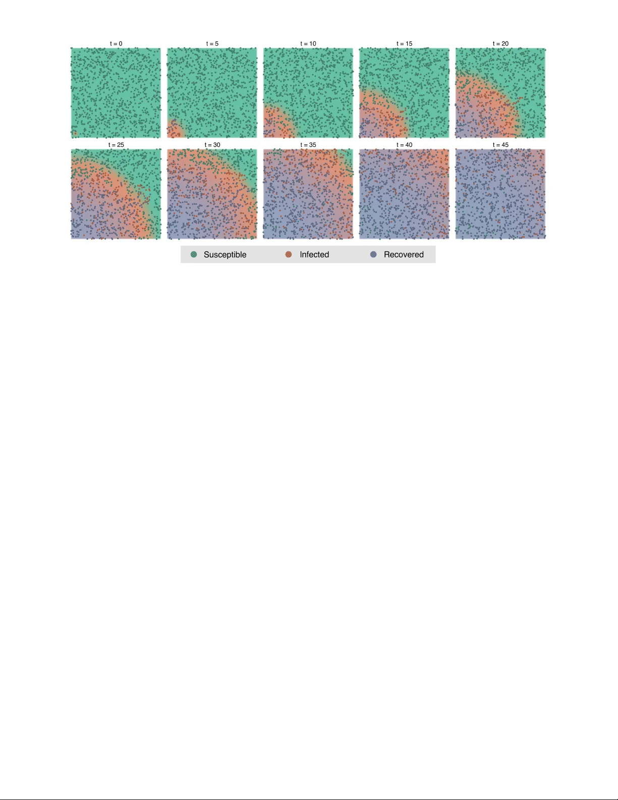
Co x pro cess represen tation and inference for sto c hastic reaction-diﬀusion pro cesses Da vid Sc hno err 1,2,3 , Ramon Grima 1,3 , and Guido Sanguinetti 2,3,* 1 Sc ho ol of Biological Sciences, Universit y of Edinburgh, Edin burgh EH9 3JH, UK 2 Sc ho ol of Informatics, Univ ersity of Edin burgh, Edin burgh EH8 9AB, UK 3 Syn thSys, Univ ersity of Edin burgh, Edin burgh EH9 3JD, UK * gsanguin@inf.ed.ac.uk August 23, 2016 Abstract Complex b eha viour in man y systems arises from the sto c hastic interactions of spatially distributed particles or agen ts. Sto c hastic reaction-diﬀusion pro cesses are widely used to mo del such b eha viour in disciplines ranging from biology to the so cial sciences, yet they are notoriously diﬃcult to simulate and calibrate to observ ational data. Here we use ideas from statistical ph ysics and machine learning to provide a solution to the in verse problem of learning a sto c hastic reaction- diﬀusion process from data. Our solution relies on a non-trivial connection betw een sto c hastic reaction-diﬀusion processes and spatio-temp oral Co x processes, a well-studied class of mo dels from computational statistics. This connection leads to an eﬃcient and ﬂexible algorithm for parameter inference and mo del selection. Our approach sho ws excellent accuracy on n umeric and real data examples from systems biology and epidemiology . Our work provides b oth insights into spatio- temp oral sto c hastic systems, and a practical solution to a long-standing problem in computational modelling. Man y complex b eha viours in several disciplines originate from a common mechanism: the dynamics of lo cally in ter- acting, spatially distributed agents. Examples arise at all spatial scales and in a wide range of scien tiﬁc ﬁelds, from microscopic interactions of lo w-abundance molecules within cells, to ecological and epidemic phenomena at the continen- tal scale. F requen tly , stochasticit y and spatial heterogeneity pla y a crucial role in determining the process dynamics and the emergence of collective b eha viour [1]-[8]. Sto c hastic reaction-diﬀusion pro cesses (SRDPs) consti- tute a con venien t mathematical framework to mo del such systems. SRDPs w ere originally introduced in statisti- cal physics [10, 11] to describ e the collective b ehaviour of p opulations of p oin t-wise agents performing Bro wnian dif- fusion in space and sto c hastically interacting with other, nearb y agen ts according to pre-deﬁned rules. The ﬂexi- bilit y aﬀorded by the lo cal interaction rules has led to a wide application of SRDPs in man y diﬀerent scientiﬁc dis- ciplines where complex spatio-temp oral b eha viours arise, from molecular biology [4, 9, 12], to ecology [13], to the so cial sciences [14]. Despite their p opularit y , SRDPs p ose considerable chal- lenges, as analytical computations are only p ossible for a handful of systems [8]. Th us, many analytical techniques whic h are widely used for non-spatial sto c hastic systems cannot b e used for SRDPs. F rom the practical p oin t of view, p erhaps the single most imp ortan t outstanding prob- lem is inference in SRDP models: giv en observ ations of the system, can w e reconstruct the in teraction rules/ lo cal dy- namic parameters? Solving this in verse problem would b e imp ortan t, as it w ould allow to quantitativ ely assess mo del ﬁt to data and to compare diﬀeren t mo dels/ hypotheses in the light of observ ations. SRDPs are generally analysed by either Brownian dy- namics simulations of individual particles, or b y resorting to spatial discretisation, leading to the so-called “reaction- diﬀusion master equation” (RDME) [15, 16]. The computa- tional complexity of the RDME ob viously increases as the spatial discretisation b ecomes ﬁner, and in man y cases the limiting pro cess do es not lead to the original SRDP [17]. Signiﬁcan t eﬀort has b een spent to impro v e the p erformance of the t w o t yp es of sim ulations [18]-[24], how ev er the compu- tational costs are still high and quickly b ecome prohibitiv e for larger systems. More imp ortan tly , the lac k of an analyt- ical alternative to sim ulations means that ev aluating the ﬁt of a mo del to observ ations (the lik eliho od function) is com- putationally extremely expensive, eﬀectively ruling out sta- tistical analyses. As far as w e are a ware, the few attempts at statistical inference for SRDPs either used sim ulation-based lik eliho o d free metho ds [13], inheriting the intrinsic com- putational diﬃculties discussed ab ov e, or abandoned the SRDP framew ork by adopting a coarse space discretisation [25] or neglecting the individual nature of agents using a linear-noise approximation [26]. In this pap er, we prop ose an approximate solution to the problem of computing the likelihoo d function in SRDPs, th us pro viding a principled solution to the in verse problem of mo del calibration. Using the classical theory of the Pois- son represen tation (PR) for sto c hastic reaction pro cesses [27], we show that marginal probability distributions of 1 SRDPs can b e approximated in a mean-ﬁeld sense by spatio- temp oral Co x p oin t processes, a class of models widely used in spatio-temporal statistics [30]. Cox processes mo del the statistics of p oin t patterns via an unobserv ed intensit y ﬁeld, a random function which captures the lo cal mean of the observ ed p oin t process. This relationship betw een SRDPs and Co x processes is surprising, as SRDPs are mechanistic, microscopic descriptions of spatio-temp oral systems, while Co x pro cesses are emplo yed phenomenologically to explain regularities in point patterns. This nov el link betw een these t wo classes of models enables us to formally associate an SRDP with a contin uous ev olution equation on the lo cal statistics of the pro cess in terms of (sto c hastic) partial dif- feren tial equations (SPDEs). Crucially , this nov el repre- sen tation of SRDPs allows us to eﬃcien tly approximate m ultiple-time marginals and thus data lik eliho o ds asso ci- ated with observed point patterns, enabling us to lev erage the ric h statistical literature on spatio-temporal p oin t pro- cesses for parameter estimation and/or Bay esian inference [30, 31]. W e demonstrate the eﬃciency and accuracy of our ap- proac h for the problem of parameter inference and mo del selection by means of a num b er of numerical and real data examples using non-trivial models from systems biology and epidemiology . Our results provide both a v aluable resource for p erforming statistical inference and assessing model ﬁt in this imp ortan t class of mo dels, and a nov el conceptual p erspective on spatio-temporal stochastic systems. Results SRDPs and the Poisson representation. In the classi- cal Doi in terpretation [10, 11], whic h we adopt here, SRDPs describ e the ev olution of systems of p oint particles p erform- ing Brownian diﬀusion in a spatial domain D . While SRDPs are used in a v ariety of disciplines, we will use the language of c hemical reactions to describe them in the follo wing. W e assume the existence of N diﬀerent t yp es of particles X i , or sp ecies, which can interact through a set of pre-deﬁned rules, or reactions. W e assume the structure of the model, i.e. which reactions are p ossible, to b e known exactly; later w e will relax this assumption to allo w for the existence of a (ﬁnite) num b er of p ossible alternativ e mechanisms. Each particle of a particular sp ecies X i p erforms Bro wnian dif- fusion with a sp ecies-sp eciﬁc microscopic diﬀusion constant D i . Bimolecular reactions b et ween particles o ccur with a certain rate whenev er t wo particles are closer than some sp eciﬁed reaction range. In principle, b oth reaction and microscopic diﬀusion rate constan ts ma y be space dep en- den t, for example to accoun t for geometric constrain ts; for simplicit y , we will only describe the homogeneous case here. SRDPs are frequently analysed via coarse graining by dis- cretising space and ass uming dilute and well-mixed condi- tions in each compartmen t; in this case the dynamics in eac h compartment is describ ed b y the chemical master equa- tion [32]. Mo delling diﬀusion of particles b et ween neigh- b ouring compartments as unimolecular reactions leads to the reaction-diﬀusion master e quation (RDME) [15], which describ es the dynamics of a contin uous-time Marko v jump pro cess. F or systems with only zeroth or ﬁrst order reac- tions, the RDME conv erges to Brownian dynamics in the con tinuum limit. F or non-linear systems, how ever, this is not the case in t wo or more dimensions b ecause the rate of bimolecular reactions conv erges to zero, independently of the scaling of the corresp onding rate constant [17]. Consider no w a set of chemical species X i in a ﬁnite v ol- ume divided into L cubic compartments of edge length h in teracting via the follo wing R reactions: N X i =1 s ij X l i k j − − − − − → N X i =1 r ij X l i , j = 1 , . . . , R, l = 1 , . . . L, (1) X l i d i − − − − − → X m i , m ∈ N ( l ) , l = 1 , . . . L. (2) Here s ij and r ij are the num b er of reactants and pro duct particles of species X i in the j th reaction, resp ectiv ely , k j is the rate constant of the j th reaction, X m i denotes species X i in the m th compartmen t, and d i is the diﬀusion rate con- stan t of species X i . The latter is related to the microscopic diﬀusion constant D i via d i = D i /h 2 . W e assume homoge- nous diﬀusion here, i.e., d i is indep enden t of the compart- men t position, but it would b e straightforw ard to extend the following analysis to space-dep enden t diﬀusion. N ( l ) denotes all the adjacen t compartments of the l th compart- men t. Equation (1) describ es c hemical reactions happening in single compartmen ts while Equation (2) describ es diﬀu- sion betw een adjacen t compartmen ts. W e conﬁne our anal- ysis to reactions with at most tw o reactant and at most tw o pro duct particles, i.e., P N i =1 s ir , P N i =1 r ir ≤ 2 , r = 1 , . . . , R , since higher order reactions rarely o ccur in nature. W e call a reaction linear if P N i =1 s ir , ≤ 1 and bimolecular if P N i =1 s ir , = 2. Under w ell-mixed and dilute conditions in eac h compartment, the evolution of marginal probabilities of this system is giv en b y the RDME which is given in gen- eral form in the Metho ds section. In the case of only a single compartmen t, i.e., L = 1, the state of the system is given by n = ( n 1 , . . . , n N ), where n i is the num b er of X i particles in the system, and the time ev olution of the single-time probability distribution P ( n , t ) is determined b y the chemical master equation (see Methods section). Gardiner deriv ed an alternativ e description of the dynamics of such a system b y making the ansatz of writing P ( n , t ) as a Poisson mixture [27, 28]: P ( n , t ) = Z d u N Y i =1 P ( n i ; u i ) p ( u , t ) , u i ∈ C , (3) where u = ( u 1 , . . . , u N ) and P ( n i ; u i ) = ( e − u i u n i i ) /n i ! is a P oisson distribution in n i with mean u i , and the u i are complex-v alued in general. Using this ansatz in the chemi- cal master equation one can deriv e an exact F okk er-Planck equation for p ( u , t ) or equiv alen tly a Langevin equation for u ( t ) [27] (see Metho ds section for more details). Gardiner derived this result for the non-spatial chemical master equation and applied it to the RDME to study the corresp onding con tinuum limit. While the PR provides 2 Figure 1: Visualisation of Cox pro cess appro ximation of SRDPs for m ulti-time p oints. (a) Time ev olution of the true SRDP in space. Particles diﬀuse in space, ma y decay or are created and react with each other. (b) Time ev olution of a Cox process. Here, the intensit y ﬁeld evolv es in time, rather than the p oin ts in real space. The latter are merely noisy realisations of the intensit y ﬁeld. In particular, the p oin ts patterns at tw o diﬀerent time p oin ts are indep enden t of each other conditioned on the intensit y ﬁeld. an elegant analytical to ol to study reaction systems, its applicabilit y is sev erely hindered b y the fact that the P oisson v ariables u are in general complex-v alued and hence lack a clear physical interpretation; in particular, all bimolecular reactions and all linear reactions with t wo non- iden tical pro duct particles give rise to a complex-v alued PR (for a taxonomy of whic h reaction systems become complex-v alued see Appendix A.1). Co x process represen tation. While in the classical view of the PR the auxiliary v ariables u i are simply introduced as a mathematical device, we can make some progress by considering a joint pro cess ov er the u i and n i v ariables. F ormally , this is equiv alent to what in statistics is called demarginalisation: a complex pro cess is replaced b y a (sim- pler) pro cess in an augmented state space, such that the marginals of the augmen ted process return exactly the ini- tial process. T o formalise this idea, w e ﬁrst in tro duce some concepts from spatial statistics. A (spatial) Poisson pro cess [29] is a measure on the space of zero-dimensional subsets of a domain D ; in this work w e consider Poisson pro cesses which admit an in tensity function u ( x ), which giv es the rate of ﬁnding a point in an inﬁnitesimally small spatial region. The n umber of p oin ts in a ﬁnite spatial region is then a Poisson random v ariable with mean given by the in tegral of the in tensity function ov er that region. A Cox pro cess (also called “doubly sto c hastic P oisson pro cess”) is a generalisation of a P oisson pro cess where the intensit y ﬁeld is itself a random pro cess. Conditioned on a realisation of the in tensity ﬁeld, the Cox process reduces to a Poisson pro cess (see Metho ds section for a more detailed deﬁnition of P oisson and Co x pro cesses). W e will consider families of spatial P oisson (Co x) pro cesses indexed by a time v ariable; imp ortan tly , in this case the in tensity ﬁeld can b e thought of as the state v ariable of the system, with the actual spatial points being noisy realisations of this state (see Fig. 1 for a graphical explanation). Our ﬁrst observ ation follows directly from Gardiner’s analysis of the con tinuum limit of the RDME (see App endix A.3 for a pro of ). Remark 1. Consider an SRDP on a spatial domain D and temporal domain T , and let all reactions inv olve pro duction or decay of at most one particle. Then, for appropriate initial conditions, ∀ t ∈ T the single-time-p oin t spatial probabilit y distribution of the SRDP is exactly the same as of a spatial P oisson pro cess. General SRDPs. W e can build on this point pro cess rep- resen tation to develop nov el, mathematically consistent ap- pro ximation sc hemes for SRDPs in general. Consider for example a bimolecular reaction of the t yp e A + B k − → C with propensity function f ( n A , n B ) = k n A n B / Ω, where n A and n B are the n umber of A and B particles in the sys- tem, resp ectiv ely , and Ω is the system volume. While the PR for such systems is complex-v alued, we can formally obtain a real system by applying a mean-ﬁeld approxima- tion that replaces the bimolecular reaction A + B k − → C b y the tw o reactions A k h n B i / Ω − − − − − − → C and B k h n A i / Ω − − − − − → C with prop ensity functions f ( n A , n B ) = kn A h n B i / Ω and f ( n A , n B ) = k n B h n A i / Ω, resp ectiv ely . Here, h·i denotes the exp ectation of a random v ariable with resp ect to its marginal distribution. The prop osed approximation hence replaces the direct in teraction of the particles by an eﬀec- tiv e in teraction of A with the mean-ﬁeld of B and vice v ersa. Other bimolecular reactions and linear reactions with t wo non-iden tical pro duct particles can b e approximated in a similar fashion. This leads to a real-v alued ev olution equa- tion for the u i v ariables, see Methods and App endix A.2 for details and examples. 3 Applying this approximation to a general RDME and sub- sequen tly the PR and taking the con tinuum limit giv es the follo wing set of N coupled SPDEs (see Methods section for a deriv ation) du i ( x, t ) = [ D i ∆ u i ( x, t ) + R X r =1 S ir g r ( u ( x, t ))] dt + X r 0 p 2 g r 0 ( u ( x, t )) dW r 0 ( x, t ) , (4) where the sum ov er r 0 runs ov er all reactions with tw o pro duct particles of sp ecies X i . In particular, this means that in the absence of reactions with tw o iden tical pro d- uct molecules the diﬀusion term in Equation (4) v anishes and Equation (4) reduces to a partial diﬀerential equa- tion (PDE), i.e., the u i ( x, t ) are deterministic. x in Equa- tion (4) is a spatial lo cation, D i = h 2 d i is the microscopic diﬀusion constan t of sp ecies X i , ∆ is the Laplace op era- tor, u ( x, t ) = ( u 1 ( x, t ) , . . . , u N ( x, t )), u i ( x, t ) is the in tensity ﬁeld of sp ecies X i , dW r 0 ( x, t ) is spatio-temp oral Gaussian white noise, and we hav e deﬁned the prop ensit y functions g r ( u ( x, t )) in PR space. The latter are obtained b y apply- ing the mean-ﬁeld approximation to the prop ensit y func- tions f r ( n ) and subsequently replacing n i → u i ( x, t ) and h n i i → h u i ( x, t ) i . Note that the latter denotes a lo cal exp ec- tation of the stochastic random ﬁeld u i ( x, t ), rather than a spatial av eraging. See Metho ds and Appendix A.2 for more details and examples. In order to obtain Equation (4) w e appro ximated bimolec- ular reactions by linear reactions. Note how ev er that the prop ensit y functions of the latter reactions dep end on the mean ﬁelds of certain sp ecies. This means that the resulting SPDEs in Equation (4) are generally non-linear and hence in principle able to capture non-linear dynamical behaviours. Equation (4) lo oks similar to the spatial chemical Langevin equation [33], but has a diﬀerent interpretation here since it describes the intensit y in PR space. In particular, just as any other PDE or SPDE description in real space, the spatial chemical Langevin equation do es not provide a generativ e mo del for the actual location of the even ts, and thus would not allow us to directly mo del statistically particle lo cations. Notice that, as a consequence of the mean-ﬁeld approximation, the mean v alues of the u i ﬁelds are the same as in a deterministic rate equation description; how ev er, the dynamics of the observ ed v ariable, i.e., the p oin ts in space, remain stochas- tic even when the in tensity ﬁeld evolv es deterministically . W e can therefore extend Remark 1 to obtain the following result (see App endix A.3 for a pro of ) Result 1. Consider the same setting as in Remark 1. Under appropriate initial conditions, if there is at least one linear reaction with t wo pro duct particles of the same species, the system’s single-time-p oint distribution is exactly the same as of a Co x process, whose intensit y fulﬁls the stochastic PDE (SPDE) given in Equation (4). If the system inv olves other t yp es of reactions, including bimolec- ular reactions, the single-time probability distribution of the SRDP is appro ximated in a mean-ﬁeld sense b y that of a P oisson (Co x) process whose in tensit y fulﬁls Equation (4). The lik eliho o d function. Result 1 pro vides an eﬃcient means to calculate statistics such as expected n umber of agen ts within a certain volume, without the need to perform extensiv e Mon te Carlo simulations, since it only requires to solve a (S)PDE for which a ric h literature of numerical metho ds exists [30, 31]. The n umerical methods used in this pap er are presented in the App endix B. Importantly , w e can use Result 1 to approximate the likelihoo d function of a conﬁguration of p oin ts arising from an SRDP , b y using the w ell-known Co x pro cess likelihoo d: if u ( x, t ) is the in tensit y of a spatio-temporal Cox pro cess with distribution p ( u ( x, t )) and y a given measurement at time t 0 , the corresp onding lik eliho o d is giv en by [30] p ( y ) = Z D u ( x, t ) Y s ∈ y u ( s, t 0 ) e − R dxu ( x,t 0 ) p ( u ( x, t )) . (5) This function can b e easily optimised to yield statistical es- timates of kinetic parameters from single-time observ ations. Remark 2. W e w ould lik e to emphasise that in the case of a Co x pro cess, i.e., a sto c hastic in tensity ﬁeld, the n umber of particles in t wo non-o verlapping spatial regions are correlated random v ariables in general. The reason is that the PR ansatz in Equation (3) is not merely a pro duct of P oisson distributions, but rather an integral ov er suc h a pro duct w eighted by a corresp onding mixing distribution. In the case of a P oisson pro cess, i.e., a deterministic in tensity ﬁeld, in contrast, the n umbers of particles in t wo non-o verlapping spatial regions are alwa ys uncorrelated. Time-series observ ations. W e consider next the prob- lem of appro ximating the joint distribution of point patterns arising from an SRDP at diﬀerent time points. This is im- p ortan t when w e hav e time -series observ ations, i.e., spatial measuremen ts y = ( y t 0 , . . . , y t n ) , y t i ⊂ D at discrete time p oin ts t 0 , . . . , t n , and we wan t to compute the likelihoo d p ( y | Θ) of the data giv en a mo del Θ. Since the system is Mark ovian the lik eliho o d factorises as p ( y | Θ) = p ( y t 0 | Θ) n Y i =1 p ( y t i | y t i − 1 , Θ) . (6) W e would like to approximate this likelihoo d using the relation to Co x pro cesses established in Result 1. While this is in principle straightforw ard, computing the terms p ( y t i | y t i − 1 , Θ) inv olves determining the distribution ov er the asso ciated u i ( x, t ) ﬁelds in PR space. This would in volv e inv erting the PR transformation in Equation (3), whic h is computationally inconv enient. Instead, we opt for an approximation strategy: assume that we hav e determined the PR distribution p ( u t i − 1 ) at time t i − 1 , where we introduced the shorthand u t i = u ( x, t i ). By deﬁnition of the intensit y of a Poisson process, u t i − 1 represen ts the e xpectation of the random conﬁguration of p oin ts y t i − 1 at time t i − 1 . W e then approximate p ( y t i | y t i − 1 , Θ) in a mean-ﬁeld w a y b y replacing the explicit 4 dep endence on y t i − 1 with its expectation p ( y t i | y t i − 1 , Θ) ≈ h p ( y t i | y t i − 1 , Θ) i p ( y t i − 1 | u t i − 1 ) = p ( y t i | u t i − 1 , Θ). Fig. 1 visualises this approximation. Fig. 1a shows the time ev olution in an SRDP , while Fig. 1b sho ws the time ev olution of a corresp onding approximating Cox pro cess. This leads to a new interpretation of the measured points y = ( y t 0 , . . . , y t n ): while they are snapshots of the actual state in the true system, they corresp ond to noisy realisa- tions of the state u ( x, t ) in the Co x process picture. W e th us hav e Result 2. The join t n -time-p oin t marginal distribution of an SRDP can b e approximated in a mean-ﬁeld sense by the join t probabilit y of a P oisson (Co x) process with intensit y go verned b y the (S)PDE in Equation (4). Relation to Gardiner’s work. As men tioned b efore, Gardiner had already derived similar equations as Equa- tion (4) for single-time marginals of SRDPs [27]. Crucially , ho wev er, an approximation sc heme for multiple-time join t marginals was, to our knowledge, never prop osed; m ulti-time join t marginals are necessary for inference from time-series observ ations, hence the imp ortance of Result 2. F urthermore, Gardiner’s approac h generally leads to a complex-v alued PR; this motiv ates the nov el appro ximation schemes of certain reactions that we in- tro duced here. It is this no vel real-v alued PR, together with the in terpretation of the PR v ariables as state v ariables, whic h allows us to derive the nov el relation b e- t ween SRDPs and spatio-temporal P oisson (Cox) processes. Inference. Result 2 is particularly p o werful statistically , b ecause it enables us to analytically appro ximate the ex- act (intractable) likelihoo d p ( y | Θ) in Equation (6) by the lik eliho o d of a spatio-temp oral Co x pro cess with in tensity u ( x, t ). The in tensity itself follows the dynamics imp osed b y the Poisson representation in Equation (4); imp ortantly , the Poisson representation explicitly links the dynamic pa- rameters gov erning the evolution of the intensit y function to the microscopic diﬀusion and reaction rate constan ts of the SRDP . P arameter estimation can therefore b e p erformed eﬃ- cien tly by maximising the Cox pro cess lik eliho o d. In the simpler case where the in tensity function evolv es determin- istically , the likelihoo d can be ev aluated numerically via the solution of a system of PDEs, and the dynamic parameters can b e numerically recov ered using standard optimisation algorithms. In the case where the intensit y function evolv es sto c hastically , we ev aluate the likelihoo d b y an approximate ﬁltering approach, as commonly used in man y statistical and engineering applications (see App endix B for algorith- mic details). The a v ailabilit y of a lik elihoo d function enables us to pro- vide a statistically meaningful, data-driven assessmen t of ho w well a mo del describ es the data. This is particularly imp ortan t when there is uncertaint y as to the precise mecha- nism underlying the data, e.g. the exact reactions or sp ecies in volv ed. Likelihoo d estimates, appropriately penalised to Figure 2: Gene expression system. (a) Chemical re- actions taking place. (b) Illustration of system in a one- dimensional cell. The mRNA b ecomes transcrib ed in the n ucleus, and b ecomes translated to proteins in the cytosol. mRNA and protein molecules decay sto c hastically and un- dergo Brownian diﬀusion across the whole cell. accoun t for model complexit y , can then b e used to select mo dels according to their supp ort from the data. It is imp ortant to notice that our approach directly opti- mises the kinetic parameters of the model, rather than ﬁt- ting an intensit y function to the observed points and then ﬁtting the dynamics. Since kinetic parameters are usually m uch fewer than the n umber of observ ations av ailable, the risk of ov er-ﬁtting is generally low in our approach. Next, we apply Result 1 and Result 2 to several ex- amples, and p erform parameter inference by maximising the data likelihoo d. W e solv e the corresp onding (S)PDEs n umerically b y pro jecting them onto a ﬁnite set of spatial basis functions, see App endix B.1 for details. P arameter estimation for a gene expression system. T o demonstrate the accuracy of our metho d, w e ﬁrst con- sider simulated time-series data in this section. Consider a gene expression system as illustrated in Fig. 2. F or sim- plicitly , we consider a one-dimensional version of this sys- tem here with the nucleus lo cated at one side of the cell. A gene lo cated in the nucleus is transcribed into mRNA molecules. The latter decay and diﬀuse across the whole cell and are translated in to proteins in the cytosol. The pro- tein molecules also diﬀuse across the whole cell and deca y . F or simplicity , we do not model the gene explicitly but as- sume that mRNA b ecomes transcrib ed with a certain ﬁxed rate m 1 homogeneously in the nucleus. The corresp onding 5 T able 1: Inference results for gene expression system. The table sho ws the inferred parameter v alues for the gene expression system illustrated in Fig. 2 with reactions in Equations (7) and (8). W e assume measurements of the protein while the mRNA is unobserved. The inference is carried out b y maximising the likelihoo d of simulated data for thirty measuremen t points separated b y ∆ t = 0 . 5. This procedure is carried out for h undred sim ulated data sets, and the mean v alue and standard deviation (in parenthesis) of the inferred results are display ed. r d m d p m 1 m 2 p 1 p 2 exact 0 . 3 0 . 1 0 . 1 20 0 . 5 20 0 . 2 inferred 0.31 (0.06) 0.12 (0.08) 0.14 (0.06) 23 (12) 0.51 (0.4) 26 (18) 0.25 (0.1) T able 2: Inference results for gene expression system with additional auto catalytic reaction. The table shows the inferred parameter v alues for the gene expression system illustrated in Fig. 2 with reactions in Equations (7) and (8) and the additional auto catalytic reaction in Equation (9). Since only the diﬀerence p 2 − p 3 is identiﬁable we ﬁx p 3 = 0 . 01 and infer the other seven parameters. The table sho ws the a verage and standard deviations (in paren thesis) of the inference results for hundred sim ulated data sets. r d m d p m 1 m 2 p 1 p 2 exact 0 . 3 0 . 1 0 . 1 20 0 . 5 20 0 . 2 inferred 0.30 (0.05) 0.14 (0.08) 0.088 (0.03) 27 (17) 0.57 (0.3) 24 (21) 0.19 (0.08) reactions are ∅ m 1 − − − − − → M , M m 2 − − − − − → ∅ , (7) M p 1 − − − − − → M + P , P p 2 − − − − − → ∅ , (8) where M and P denote the mRNA and protein, respectively . F or this system, the SPDE of our method in Equation (4) b ecomes deterministic and thus corresp onds to a Poisson pro cess. In addition to the reaction parameters m 1 , m 2 , p 1 and p 2 , w e hav e to infer the nucleus size r , as w ell as the diﬀusion rates d m and d p of the mRNA and protein, resp ectiv ely , summing up to a total n umber of seven parameters. W e assume that the p ositions of the protein molecules are ob- serv ed at thirt y time p oin ts, while the mRNA is unobserved. The results for one parameter set are shown in T able 1. Considering that w e observ e the protein at only thirty time p oin ts with unobserv ed mRNA and that we hav e sev en un- kno wn parameters, the inferred av erage v alues are remark- ably close to the exact v alues. Moreov er, the standard de- viations of the inferred results for single data sets are small, demonstrating the accuracy and precision of our metho d. Next, w e extend the system in Fig. 2 by adding an auto- catalytic reaction for the protein, P p 3 − − − − − → P + P. (9) Including this reaction leads to a non-v anishing noise term in Equation (4) and the system corresp onds to a Cox pro cess. W e note that the system has a steady state only if p 3 < p 2 , with an otherwise exp onentially growing mean protein num ber. On the mean level only the diﬀerence p 2 − p 3 is identiﬁable, and w e ﬁx p 3 = 0 . 01. W e thus infer the same parameters as in the previous case, but this time modelled as a Cox pro cess. T able 2 shows the results indicating the accuracy of our metho d. See App endix C.1 for more information on the used equations and algorithmic details. P arameter estimation for an SIRS mo del. W e next consider the SIRS system, a p opular model for describing the dynamics of an infection spreading through a p opula- tion. Such systems are frequen tly mo delled as SRDPs [34] or discretised versions thereof [35]. W e consider a system in the tw o-dimensional square [0 , 1] × [0 , 1]. The system comprises a susceptible (S), an infected (I) and a reco vered sp ecies (R), whic h p erform Brownian diﬀusion and in teract via the reactions S + I k,w − − − − − − → 2 I , I r − − − − → R , R s − − − − → S, (10) where the bimolecular infection is characterised by the mi- croscopic reaction rate k and the reaction range w . W e assume that all three sp ecies diﬀuse with the same diﬀu- sion rate d . W e assume further that initially there are no reco vered (R) particles, S ini susceptible (S) particles placed uniformly o v er the whole area, and one infected (I) particle lo cated at [0 . 05 , 0 . 05]. W e consider the case that all three sp ecies are observ ed and p erform inference for fort y sim u- lated data p oints using Result 2, thereby replacing k and w by an eﬀective bimolecular reaction parameter k PR . The mo del thus has four parameters that need to b e inferred: the diﬀusion rate d , the recov ery rate r , the susceptible rate s and the bimolecular infection rate k PR . T able 3 shows the corresp onding results, demonstrating the accuracy and precision of our metho d. The computational eﬃciency of our metho d in comparison to stochastic simulati ons is par- ticularly pronounced here. F or the ﬁrst parameter set in T able 3, for example, the Brownian dynamics simulation of a single realisation of the system takes about 250 seconds, while the whole inference pro cedure for the four parameters App endix C.2 for more details. Fig. 3 visualises the dynamics of the SIRS system for one parameter set. Individual points from a simulation are sho wn in diﬀerent colours (turquoise for S, bronze for I and blue for R), while the background RGB colours represent a sup erposition of the resp ectiv e intensit y ﬁelds with optimised parameters. Notice ho w the PR approximation 6 t = 0 t = 5 t = 10 t = 15 t = 20 t = 25 t = 30 t = 35 t = 40 t = 45 Figure 3: Dynamics of SIRS system. The ﬁgure sho ws the time ev olution of a single sim ulated realisation (points) and of the prediction of our metho d (background colours) for the SIRS system with reactions in Equation (10) for time t = 0 to t = 45 with steps of ∆ t = 5. F or the sim ulation we use the parameters ( S ini, k , w , d, r, s ) = (10 3 , 10 4 , 0 . 02 , 0 . 0002 , 0 . 3 , 0 . 01) and for the p oin t process prediction the corresponding inferred parameters. The background is an RGB image with the three colour comp onen ts b eing prop ortional to the intensit y ﬁelds of the three sp ecies S (turquoise), I (bronze) and R (blue). Notice how the mean-ﬁeld appro ximation captures the complex b eha viour of a w a ve of infection spreading through the domain from the b ottom left corner. is able to capture the emerging b eha viour of a wa v e of infection sw eeping through the domain from bottom left to top righ t, b efore the establishment of a dynamic equilib- rium b etw een the three p opulation. Suc h a phenomenon is clearly due to the spatial asp ect of the system, and could not hav e b een recov ered using an inference metho d that do es not incorporate spatial information. Indeed, the o verall num b er of infected individuals rises rapidly and remains essentially constant b et ween time 20 and time 35 b efore dropping to steady state, a behaviour which is simply not p ossible in a non-spatial SIRS model. P arameter estimation for Drosophila embry o data. Finally , w e apply our method to real gene expression data for the Bicoid protein at clea v age stage 13 in the Drosophila em bryo. The data for sev enteen embry os can b e obtained from the FlyEx database [37]. The data consists of ﬂuores- cence in tensity measurements on a spatial grid and is shown for one em bryo in Fig. 4a. The protein becomes expressed in some region at the left end of the em bryo and then dif- fuses across the em bryo and deca ys. The system is typically mo delled b y a linear birth-death pro cess [25, 26], and w e as- sume the protein to b e expressed within a certain distance r from the left end of the em bry o. A t cleav age stage 13 the system is supp osed to be in steady state and w e can p erform inference using Result 1 and Equation (4). F or simplicity , w e pro ject the data to one dimension (see App endix C.3 for more details). The system has four parameters: the creation range r , the diﬀusion rate d , the pro duction rate c 1 and decay rate c 2 of the Bicoid protein. F or steady-state data not all parameters but only certain ratios are identiﬁable. W e thus infer the creation range r , the diﬀusion rate d and the ratio c = c 1 /c 2 . F or the av erage of the inferred parameters and their standard deviations (shown here in paren theses) across the ensem ble of em bryos w e obtain r = 0 . 26(0 . 09) , d = 0 . 023(0 . 005) , c = 1 . 3(0 . 2) × 10 4 , (11) with standard deviations of ab out 20% to 30%. W e ﬁnd that these results do not c hange signiﬁcan tly under v ariations of the ini tial parameter v alues used in the lik eliho o d optimiser. Fig. 4 illustrates the inference result for one embry o. Figs. 4a and 4b show the Bicoid density across the whole em bryo for exp erimen tal data and the PR prediction, resp ectiv ely . W e observe goo d agreement b et ween the measuremen t data and the p oin t pro cess appro ximation. Fig. 4c sho ws a plot of the mo del residuals (diﬀerence b et w een model predictions and real data); as can b e seen, these are generally comparatively small. As could b e exp ected, the larger errors are concentrated around the steeply changing gradien t region b et ween the anterior segmen ts and the main b ody of the em bryo. Mo del selection for an SIRS mo del. Next, we use Result 2 to p erform mo del selection. Sp eciﬁcally , we use our metho d to decide whic h of t wo given microscopic mo dels is more lik ely to b e the true mo del underlying some giv en 7 T able 3: Inference results for SIRS system. The table shows the results for parameter inference for the SIRS sys tem with reactions giv en in Equation (10). The inference is carried out b y maximising the lik eliho od of simulated data for fort y measurement points. This pro cedure is carried out for tw o hundred simulated data sets, and the mean v alue and standard deviation (in parenthesis) of the inferred results are displa yed. 10 3 × d 10 × r 10 × s 10 3 × k PR k w S ini exact 1 0.2 2 - 100 0.01 200 inferred 0.8 (0.3) 0.19 (0.09) 1.8 (1.2) 2.5 (0.5) - - exact 1 0.2 2 - 100 0.01 300 inferred 0.9 (0.4) 0.15 (0.06) 1.4 (0.9) 2.4 (0.5) - - exact 1 2 2 - 100 0.02 200 inferred 1.0 (0.6) 1.6 (0.7) 1.5 (1.0) 3.4 (1.1) - - exact 1 0.2 2 - 1000 0.005 200 inferred 0.8 (0.4) 0.21 (0.11) 2.2 (1.6) 2.4 (0.5) - - exact 2 0.2 2 - 100 0.01 100 inferred 1.6 (0.8) 0.19 (0.09) 1.9 (1.2) 4.6 (1.1) - - a b c Bicoid data Model prediction Residuals Fluoresence intensity Intensity difference 50 100 150 200 -25 -5 15 35 Figure 4: Results for the Drosophila em bryo Bicoid data. (a) Measuremen t data of Bicoid ﬂuorescent in tensity across a single embry o. (b) Corresp onding prediction of our p oin t pro cess mo del. (c) Diﬀerence of the exp erimental data and p oint pro cess prediction. W e observ e the p oint pro cess prediction agrees well with the exp erimental data. The point pro cess prediction is obtained by solving Equation (4) n umerically for the inferred parameter v alues maximising the data lik eliho o d. data set. T o this end, we use the Bay esian information criterion (BIC) [38]. The BIC for a model is the negativ e log-lik eliho o d p enalised b y a term depending on the num b er of inferred parameters and n umber of measurement p oin ts. The mo del with the low er BIC is then chosen to b e the true mo del. As an example, we mo diﬁed the SIRS model of Equa- tion (10) b y including the p ossibility of a spontaneous, spa- tially homogeneous infection of susceptible agents, accord- ing to the reaction S v − − − − → I . (12) W e consider tw o scenarios: the true microscopic model used to generate the data do es or do es not contain the sponta- neous infection reaction. In either case, we use our metho d to select the true model. T o this end, w e optimise the lik e- liho od with respect to the parameters using our method for b oth mo dels, and compare the corresponding BICs. Figs. 5a and 5b show the results for the tw o scenarios of true mo del without and with sp on taneous infection, resp ectiv ely . The ﬁgures show how often our metho d selected the righ t or wrong mo del, and with which conﬁdence lev el. Each of the ﬁgures sho ws the com bined results for ﬁv e diﬀerent parame- ter sets and t wen ty indep enden t simulations for eac h param- eter set. W e ﬁnd that our metho d c hose the correct model in the v ast ma jority of the cases (89% where the true system do es not include sp ontaneous infection and 96% where the true system do es con tain sp on taneous infection.). Moreov er, our method choses the correct mo del with a “v ery strong” conﬁdence in most of the cases. This sho ws that our metho d is w ell suited for the problem of mo del selection. The eﬀec- tiv eness of our mo del selection approach is remark able, since the t w o mechanisms (sp on taneous infection and contact in- fection) can lead to iden tiﬁability problems. Such problems are particularly acute when spatial heterogeneities even out rapidly , as in the case of fast diﬀusion: the few mistak es that our model selection approach makes are primarily due to random samples of the SRDP when the infection spreads particularly fast, so that, for most time points, the pro cess is eﬀectively equilibrated. 8 a b Without spontaneous infection With spontaneous infection Wrong Correct Wrong Correct very strong strong neg. very strong weak weak pos. strong very strong strong neg. very strong weak weak pos. strong 100 80 60 40 20 0 100 80 60 40 20 0 Figure 5: Mo del selection results for SIRS system. W e use the Bay esian information criterion (BIC) for mo del selection for the SIRS system with reactions in Equation (10) and the additional sp on taneous infection reaction in Equation (12). The sign of the diﬀerence in the BIC num b ers of the t wo mo dels determines if the correct model is selected, and the corresp onding magnitude how conﬁdent this choice is. W e simulated tw en ty exp erimen ts for ﬁve parameter sets each. The ﬁgures sho w the com bined results of these hundred exp erimen ts. (a) The true system used to generate the data do es not include spontaneous infection. The parameter sets are the same as in T able 3. (b) The true system used to generate the data do es include sp on taneous infection. The parameter sets are the same as in T able 3 but with modiﬁed bimolecular infection rate whic h we set to k = 10 , 5 , 10 , 100 and 10, resp ectiv ely . The spontaneous infection rate is set to v = 0 . 002 for all parameter sets. In b oth cases, we observ e that our metho d selects the correct mo del in more than 80% of the cases, and in most of these cases with “v ery strong” conﬁdence. This demonstrates the strong p erformance of our metho d for this mo del-selection problem. Discussion W e considered t wo p opular classes of mo dels for study- ing stochasticit y in spatio-temporal systems; stochastic reaction-diﬀusion pro cesses (SRDPs) and spatio-temp oral p oin t processes. The tw o classes of mo dels are both com- monly used in many disciplines such as epidemiology [14, 39] and social sciences [40], ho wev er they are widely p erceiv ed as conceptually distinct. SRDPs are microscopic, mech- anistic descriptions used to predict the dynamics of spa- tially interacting particles, whereas point pro cesses are typ- ically used empirically to p erform inference tasks for sys- tems for whic h no microscopic description exists. The tw o approac hes therefore seem to b e orthogonal to each other. Ho wev er, in this pap er w e ha ve sho wn that the t wo meth- o ds are intimately related. By using the Poisson represen- tation (PR) we established a Cox process representation of SRDPs, which is exact for certain classes of systems and appro ximate for others. This nov el represen tation enables us to apply a wide range of statistical inference methods to SRDPs, whic h has not b een possible so far. W e applied the dev elop ed metho d to sev eral example systems from systems biology and epidemiology and obtained remark ably accurate results. Since our method agrees with a deterministic rate equa- tion description on the mean level, bimolecular reactions ma y lead to deviations from the true mean, which is kno wn to b e the case in some non-spatial scenarios [36]. Since in our method distributions are giv en as real P oisson mixtures, sub-P oissonian ﬂuctuations cannot b e captured. How ev er, Gardiner sho wed that ﬂuctuations of SRDPs are dominated b y diﬀusion on small length scales and therefore Poissonian [33], which ma y explain the accuracy of our metho d. Most inference metho ds in the literature for SRDPs are either based on Brownian dynamics sim ulations or sto chas- tic simulations of spatially discretised systems using the RDME. Both approac hes are computationally extremely ex- p ensiv e and quic kly b ecome unfeasible for larger systems and in particular for inference purp oses. In con trast, our metho d relies on the solution of (S)PDEs for which a rich lit- erature of eﬃcient n umerical metho ds exists. F or the stud- ied example systems our metho d turned out to be highly ef- ﬁcien t: the computational time for inferring four unkno wn parameters for the SIRS system, for example, was found to b e of the order of 10 seconds on a 3 . 1GHz pro cessor. W e therefore exp ect our metho d to b e applicable to signiﬁ- can tly larger systems containing more sp ecies and unknown parameters. Remark ably , simulating a single realisation of the SIRS system from Bro wnian dynamics sim ulations to ok ab out an order of magnitude longer than the whole infer- ence pro cedure using our metho d, i.e., optimising the like- liho od with resp ect to the parameters, indicating the im- mense computational costs of inference metho ds based on suc h simulations. Ha ving access to a lik eliho od function also pro vides a ma- jor adv antage in handling model uncertaint y: our results on a spatial SIRS mo del show that lik elihoo d-based criteria can eﬃcien tly and accurately discriminate b et ween comp eting mo dels. This success raises the p ossibilit y that our approach could lay the foundations for structure learning of spatio- temp oral sto c hastic systems: leveraging spatially resolv ed data not only to identify parameters, but to learn directly the mec hanisms underlying the data. The av ailability of a lik eliho o d approximation mak es it in principle p ossible to 9 b orro w tec hniques from ﬁelds where structure learning is more established and where eﬃcien t netw ork learning algo- rithms based on regularised regression or random forests are routinely used, such as learning gene regulatory netw orks [41, 42]. Our approach can also readily handle spatial heterogene- it y in the reaction or diﬀusion rates: the gene regulation example sho wed that the metho d can precisely iden tify sim- ple geometric features of the system, suc h as the radius of the cell nucleus. While our examples are primarily illus- trativ e of the metho dology , and hence simple, it w ould be in principle straightforw ard to generalise the approac h to SRDPs deﬁned on complex geometries, such as the in tracel- lular landscap es rev ealed by X-ray tomograph y [43]. Learn- ing complex geometries directly from data w ould p oten tially b e more challenging, ho w ever, as it would generally require learning a large num b er of parameters. While we believe that the derived represen tation of SRDPs in terms of Co x pro cesses brings clear adv an tages from a statistical p oint of view, it is also important to ac- kno wledge the limitations implied by the employ ed mean- ﬁeld approximations. Perhaps the most imp ortant step in our appro ximation is the mean-ﬁeld treatment of m ulti-time join t distributions in Result 2. As noticed before, this re- places direct dep endencies betw een particle locations at dif- feren t time p oin ts with indirect dep endences through the in tensity ﬁeld. This implies that self-excitatory b ehaviours, suc h as clustering, cannot b e accurately captured; at best, these will be mimic ked by a lo cal increase in the intensit y ﬁeld within a Co x pro cess framework. More complex p oin t pro cesses that can accoun t for self-excitatory b eha viour do exist [44]; in our opinion, it is a question of considerable the- oretical interest whether suc h pro cesses can also arise from a dynamical SRDP representation. Metho ds The chemical master equation. Consider a system of N sp ecies X i , i = 1 , ..., N that in teract stochastically via R reaction c hannels N X i =1 s ij X i k j − − − − − → N X i =1 r ij X i , j = 1 , . . . , R, (13) where k j is the rate constant of the j th reaction and the s ij and r ij are the non-negative integer num b ers. Deﬁne the sto- ic hiometric matrix S as S ij = r ij − s ij ; the j th reaction is of order m if P N i =1 s ij = m . W e only consider reactions satisfying P N i =1 s ij , P N i =1 r ij ≤ 2, i.e., reactions with a maximum of t w o re- actan t and a maximum of tw o pro duct particles, since higher or- der reactions rarely o ccur in nature. Denote as n = ( n 1 , . . . , n N ) the state of the system, where n i is the copy num b er of species X i . Under well-mixed and dilute conditions, the time evolution of the (single-time) marginal probability distribution of the sys- tem ob eys the chemical master equation [32] ∂ t P ( n , t ) = R X r =1 f r ( n − S r ) P ( n − S r , t ) − R X r =1 f r ( n ) P ( n , t ) , (14) where S r is the r th column of the stoichiometric matrix S . The prop ensit y function f r ( n ) dt giv es the probability for the r th re- action to happ en in an inﬁnitesimal time interv al dt and is given b y f r ( n ) = k r Ω N Y k =1 n k ! ( n k − s kr )!Ω s kr . (15) Here, Ω is the volume of the system. The P oisson represen tation. The Poisson representation mak es the ansatz to write P ( n , t ) as a Poisson mixture [27] P ( n , t ) = Z d u P ( n 1 ; u 1 ) . . . P ( n N ; u N ) p ( u , t ) , u i ∈ C , (16) where u = ( u 1 , . . . , u N ) and P ( n i ; u i ) = ( e − u i u n i i ) /n i ! is a P ois- son distribution in n i with mean u i , and the u i are complex in general. The integrals in Equation (16) in general run ov er the whole complex plane for each u i . Using the ansatz (16) in the generating function equation whic h can be derived from Equa- tion (14) one can derive the following PDE for the distribution p ( u , t ) [27], ∂ t p ( u , t ) = R X r =1 Ω k r N Y i =1  1 − ∂ ∂ u i  r ir − N Y i =1  1 − ∂ ∂ u i  s ir ! × N Y j =1 Ω − s j r u s j r j p ( u , t ) . (17) Note that this PDE generally in volv es deriv ativ es of higher or- der than tw o, which means that p ( u , t ) can generally b ecome negativ e in which case it does not admit a probabilistic inter- pretation. How ever, since we only consider reactions satisfying P N i =1 s ir , P N i =1 r ir ≤ 2, Equation (17) simpliﬁes to ∂ t p ( u , t ) = − N X i =1 ∂ ∂ u i [ A i ( u ) p ( u , t )] + 1 2 N X i,j =1 ∂ ∂ u i ∂ ∂ u j [ B ij ( u ) p ( u , t )] , (18) whic h is a F okk er-Planck equation (FPE) with drift vector A ( u ) and diﬀusion matrix B ( u ) given by A i ( u ) = R X r =1 S ir g r ( u ) , (19) B ij ( u ) = R X r =1 g r ( u )( r ir r j r − s ir s j r − δ i,j S ir ) , (20) g r ( u ) = Ω k r N Y j =1 Ω − s j r u s j r j , (21) where δ i,j denotes the Kroneck er delta. The corresp onding Langevin equation reads d u = A ( u ) dt + C ( u ) d W , CC T = B , (22) where d W is a l -dimensional Wiener pro cess and l is the num ber of columns of C . Dep ending on the reactions in the system, the diﬀusion ma- trix may b e zero, in which case the Langevin equations in (22) reduce to deterministic ordinary diﬀerential equations. On the other hand, dep ending on the reactions, B ( u ) is not p ositiv e- semideﬁnite and thus CC T = B cannot b e fulﬁlled for real u , 10 whic h means that Equation (18) is not a prop er FPE in real v ariables. Rather, it needs to b e extended to complex space. Sp eciﬁcally , this is the case whenev er the system contains bi- molecular reactions or reactions with tw o non-iden tical pro duct molecules. An imp ortan t prop ert y of the PR is that the mean v alues of the particle num b ers n i are equal to the mean v alues of the corresp onding PR v ariables u i , i.e., h n i i = h u i i . The reaction-diﬀusion master equation. Consider a system as in Equation (13) but in an M − dimensional v olume discretised in to L cubic compartmen ts of edge length h and volume h M . De- note as n = ( n 1 1 , . . . , n 1 N , . . . , n L 1 , . . . , n L N ) the state of the system, where n l i is the cop y num b er of species X i in the l th compart- men t. Under w ell-mixed and dilute conditions in each compart- men t, the reaction dynamics in eac h compartmen t is go verned b y a corresp onding c hemical master equation as in Equation (14). If w e mo del diﬀusion of sp ecies X i b et w een neighbouring compart- men ts by linear reactions with rate constan t d i = D i /h 2 , where D i is the microscopic diﬀusion constan t of sp ecies X i , the time ev olution of the (single-time) marginal probabilit y distribution of the system obeys the RDME [32]: ∂ t P ( n , t ) = L X l =1 X m ∈N ( l ) N X i =1 d i [( n m i + 1) P ( n + δ m i − δ l i , t ) − n l i P ( n , t )] (23) + L X l =1 R X r =1 [ f r ( n l − S r ) P ( n − S l r , t ) − f r ( n l ) P ( n , t )] , (24) where f r ( n l ) is the prop ensit y function of the r th reaction ev aluated at the state vector n l = ( n l 1 , . . . , n l N ) of the l th compartmen t, δ l i is a vector of length N ∗ L with the entry corresp onding to sp ecies X i in the l th compartmen t equal to 1 and all other entries zero and S l r is a vector of length N ∗ L with the entries corresp onding to the l th compartmen t equal to the r th ro w of the stoichiometric matrix S and zero otherwise. Real-v alued P oisson represen tation in space. W e next ap- ply the PR to the RDME in Equations (23) and (24) after apply- ing the mean-ﬁeld approximations deﬁned in the Results section to bimolecular reactions and reactions with tw o non-identical pro duct molecules, and subsequently take the contin uum limit. Consider ﬁrst the diﬀusion term in Equation (23). Since diﬀerent sp ecies do not in teract with each other if there are no chemical reactions happening, we can consider a system con taining only a single sp ecies, say sp ecies X 1 , for which Equation (23) reduces to ∂ t P ( n , t ) = L X l =1 X m ∈N ( l ) d [( n m + 1) P ( n + δ m − δ l , t ) − n l P ( n , t )] , (25) where n = ( n 1 , . . . , n L ), n m is the num ber of X 1 particles in the m th compartmen t, δ m is a vector with a one in the m th en try and zero otherwise, d is the diﬀusion constant of sp ecies X 1 , and the sum o ver m runs ov er all neighbouring compartmen ts N ( l ) of the l th compartmen t. F or this system the PR is real and deterministic, and we use the PR without any approximations. The corresp onding Langevin equation reads du l = D 2 M u l − P m ∈N ( l ) u m h 2 dt, l = 1 , . . . , L, (26) where M is the spatial dimension of the system and D = dh 2 the microscopic diﬀusion constan t. Since the sum o ver m runs o ver all adjacen t compartments of the l th compartmen t, the fraction in Equation (26) is just the discretised versio n of the Laplace op erator ∆ = ∂ 2 1 + . . . + ∂ 2 M . In tro ducing a discretised densit y ﬁeld u ( x l ) = u l /h M , where x l is the centre of the l th compart- men t, and taking the con tinuum limit of Equation (26), we get the PDE du ( x, t ) = D ∆ u ( x, t ) dt, (27) whic h is just the diﬀusion equation for the ﬁeld u ( x, t ). Consider next the reaction term of the RDME given in Equa- tion (24). Since reactions only occur within compartmen ts, we can treat the compartmen ts indep enden tly of each other. F or a single compartment, Equation (24) then reduces to the chemi- cal master equation given in Equation (14). Here, ho wev er, w e ﬁrst apply the approximations deﬁned in the Results section to bimolecular reactions and reactions with t wo non-identical prod- uct molecules (see App endix A for more details). These approx- imations lead to a real-v alued PR and only reactions with tw o iden tical pro duct molecules lead to sto chastic terms. The PR Langevin equation hence simpliﬁes to du i = R X r =1 S ir g r ( u ) dt + X r 0 p 2 g r 0 ( u ) dW r 0 , (28) where u = ( u 1 , . . . , u N ) and the sum ov er r 0 runs ov er all reac- tions with tw o product particles of sp ecies X i . The prop ensities g r ( u ) are obtained b y replacing the n i v ariables with u i v ariables and Ω with h M in the expressions for the f r prop ensities of the appro ximated reactions. The factor of tw o in the square ro ot in Equation (28) comes from the fact that tw o iden tical molecules b ecome pro duced in these reactions. Reintroducing the lab el l denoting the compartment n umber in Equation (28), and the sp ecies lab el i in Equation (27), w e can add the t wo contributions to obtain du l i = D i 2 M u l i − P m ∈N ( l ) u m i h 2 dt + R X r =1 S ir g r ( u l ) dt + X r 0 p 2 g r 0 ( u l ) dW l r 0 , (29) where u = ( u 1 1 , . . . , u 1 N , . . . , u L 1 , . . . , u L N ) and u l i is the PR v ari- able of sp ecies X i in the l th compartmen t. If we again deﬁne discretised density ﬁelds u i ( x l ) = u l i /h M , where x l is the cen- tre of the l th compartmen t, and dW r ( x l ) = dW l r / √ h M , w e can tak e the contin uum limit of Equation (29) which leads to the real-v alued SPDE for the intensit y ﬁelds given in Equation (4). The g r ( u ( x, t )) therein are not functions of single PR v ariables an ymore, but rather functionals of the space-dep enden t in tensity ﬁeld v ector u ( x, t ) = ( u 1 ( x, t ) , . . . , u N ( x, t )). They are obtained b y taking the corresp onding propensity functions f r ( n ) of the appro ximate reactions in real space, replacing n i → u i ( x, t ) and h n i i → h u i ( x, t ) i and omitting Ω factors. The latter can b e iden- tiﬁed with h M here and hence get absorbed in the deﬁnition of the intensit y ﬁelds given b elo w Eq. (29). As an example, consider the reaction A + B → ∅ . The non-spatial propensity in real space for this reac- tion is f ( n A , n B ) = k n A n B / Ω. How ever, since this is a bimolecular reaction and hence leads to a complex- v alued PR, we replace it b y the t wo reactions A → ∅ and B → ∅ with prop ensities f ( n A , n B ) = k h n B i n A / Ω and f ( n A , n B ) = k h n A i n B / Ω, respectively . By replacing 11 n i → u i ( x, t ) and h n i i → h u i ( x, t ) i and omitting Ω terms, we th us obtain the corresp onding prop ensit y functions in spatial PR space as g 1 ( u A ( x, t ) , u A ( x, t )) = k h u B ( x, t ) i u A ( x, t ) and g 2 ( u A ( x, t ) , u A ( x, t )) = k h u A ( x, t ) i u B ( x, t ), respectively . See App endix A for more details and examples. P oisson and Cox pro cesses. A (spatial) Poisson pro cess on a spatial region D of arbitrary dimension deﬁnes a measure on coun table unions of zero-dimensional subsets (p oin ts) of D . A P oisson pro cess is often characterised by an intensit y function u : D → R + giving the probability densit y of ﬁnding a point in an inﬁnitesimal region around x . Now let N ( A ) denote the n umber of p oin ts in a subregion A ⊂ D . Then N ( A ) is a Poisson random v ariable with mean given by the integral of u ( · ) o ver A : p ( N ( A ) = n ) = P ( n ; u A ) , u A = Z A dx u ( x ) , (30) where P ( n ; u A ) is a P oisson distribution in n with mean u A . A (spatial) Cox process is a generalisation of a P oisson process and also called “doubly stochastic pro cess”, in the sense that the in tensity function u is itself a random pro cess. Conditioned on the in tensity u , the Co x pro cess reduces to a Poisson process. The distribution of the num b er of p oin ts in a subregion A ⊂ D is hence a mixture of P oisson distributions, p ( N ( A ) = n ) = Z du A P ( n ; u A ) p ( u A ) . (31) Since we are interested in dynamical systems, we will assume time-dep enden t in tensities u : D × T → R + , where T is a ﬁnite real interv al denoting time. W e then require that for an y ﬁxed time p oin t t ∈ T the pro cess is a spatial P oisson (Cox) pro cess with intensit y u ( · , t ). In the case of a P oisson (Cox) pro cess, the in tensity u may for example b e deﬁned as the solution of a PDE (SPDE). Ac kno wledgmen ts This w ork was supported by the Biotec hnology and Biologi- cal Sciences Research Council [BB/F017073/1]; the Lev erhulme T rust [RPG-2013-171]; and the European Research Council [MLCS 306999]. The authors thank Peter Swain, Andrew Zammit-Mangion, Manfred Opp er and Giulio Cara v agna for v aluable discussions and comments on the draft. References [1] Bullara, D., & De Deck er, Y. Pigmen t cell mov ement is not re- quired for generation of T uring patterns in zebraﬁsh skin. Nat. Com- mun. 6, 6971 (2015). [2] Metzler, R. The future is noisy: the role of spatial ﬂuctuations in genetic switching. Phys. R ev. L ett. 87, 068103 (2001). [3] Elf, J. & Ehren b erg, M. Sp ontaneous separation of bi-stable bio- chemical systems in to spatial domains of opposite phases. Syst. Biol. 1, 230-236 (2004). [4] T ak ahashi, K., T anase-Nicola, S. & T en W olde, P . R.Spatio- temporal correlations can drastically change the resp onse of a MAPK pathw ay . Pro c. Natl. A c ad. Sci. USA 107, 2473-2478 (2010). [5] Short, M. B., Brantingham, P . J., Bertozzi, A. L. & Tita, G. E. Dissipation and displacemen t of hotsp ots in reaction-diﬀusion mod- els of crime. Pr o c. Natl. A c ad. Sci. USA 107, 3961-3965 (2010). [6] Mahmuto vic, A., F ange, D., Berg, O. G. & Elf, J. Lost in pre- sumption: sto c hastic reactions in spatial models. Nat. methods. 9, 1163-1166 (2012). [7] Y ates, C. A. et al. Inheren t noise can facilitate coherence in col- lective swarm motion. Pro c. Natl. A c ad. Sci. USA 106, 5464-5469 (2009). [8] Cottrell, D., Swain, P . S. & T upp er, P . F. Sto c hastic branc hing- diﬀusion models for gene expression. Pr o c. Natl. A c ad. Sci. USA 109, 9699-9704 (2012). [9] Bicknell, B. A., Day an, P ., & Go odhill, G. J. The limits of chemosensation v ary across dimensions. Nat. Commun. 6, 7468 (2015). [10] Doi, M. Second quan tization representation for classical man y- particle system. J. Phys. A 9, 1465 (1976). [11] Doi, M. Sto c hastic theory of diﬀusion-controlled reaction. J. Phys. A 9, 1479 (1976). [12] Grima, R. & Sc hnell, S. A systematic in vestigation of the rate laws v alid in intracellular environmen ts. Biophys. Chem. 124, 1-10 (2006). [13] Holmes, G. R. et al. Repelled from the wound, or randomly dis- persed? Reverse migration behaviour of neutrophils characterized by dynamic mo delling. J. R. So c. Interface rsif20120542 (2012). [14] Davies, T. P ., F ry , H. M., Wilson, A. G. & Bishop, S. R. A mathematical model of the London riots and their p olicing. Sci. R ep. 3, (2013). [15] Gardiner, C. W., McNeil, K. J., W alls, D. F. & Matheson, I. S. Correlations in sto c hastic theories of chemical reactions. J. Stat. Phys. 14, 307-331 (1976). [16] F ange, D., Berg, O. G., Sj¨ ob erg, P . & Elf, J. Sto chastic reaction- diﬀusion kinetics in the microscopic limit. Pr o c. Natl. A c ad. Sci. USA 107, 19820-19825 (2010). [17] Isaacson, S. A. Relationship b et ween the reaction-diﬀusion mas- ter equation and particle tracking mo dels. Phys. Rev. Lett. 41, 065003 (2008). [18] v an Zon, J. S. & T en W olde, P . R. Sim ulating bio c hemical net- works at the particle lev el and in time and space: Green’s function reaction dynamics. Phys. Rev. L ett. 94, 128103 (2005). [19] Isaacson, S. A. & Peskin, C. S. Incorporating diﬀusion in complex geometries into sto c hastic c hemical kinetics simulations. SIAM J. Sci. Comput. 28, 47-74 (2006). [20] Erban, R. & Chapman, S. J. Sto c hastic mo delling of reaction- diﬀusion pro cesses: algorithms for bimolecular reactions. PB 6, 046001 (2009). [21] Draw ert, B., La wson, M. J., P etzold, L. & Khammash, M. The diﬀusive ﬁnite state pro jection algorithm for eﬃcient simulation of the sto chastic reaction-diﬀusion master equation. J. Chem. Phys. 132, 074101 (2010). [22] F erm, L., Hellander, A. & L¨ otstedt, P . An adaptive algorithm for simulation of stochastic reaction-diﬀusion processes. J. Comput. Phys. 229, 343-360 (2010). [23] F ranz, B., Flegg, M. B., Chapman, S. J. & Erban, R. Multi- scale reaction-diﬀusion algorithms: PDE-assisted Brownian dynam- ics. SIAM J. Appl. Math. 73, 1224-1247 (2013). [24] F u, J., W u, S., Li, H. & Petzold, L. R. The time dep endent propensity function for acceleration of spatial sto c hastic simula- tion of reaction-diﬀusion systems. J. Comput. Phys. 274, 524-549 (2014). [25] Dewar, M. A., Kadirk amanathan, V., Opp er, M. & Sanguinetti, G. Parameter estimation and inference for sto chastic reaction- diﬀusion systems: application to morphogenesis in D. melanogaster. BMC Syst. Biol. 4, 21 (2010). [26] Ruttor, A. & Opp er, M. Approximate parameter inference in a stochastic reaction-diﬀusion model. AIST A TS 669-676 (2010). [27] Gardiner, C. W. & Chaturvedi, S. The Poisson representation. I. A new technique for c hemical master equations. J. Stat. Phys. 17, 429-468 (1977). [28] Thomas, P ., Straub e, A. V. & Grima, R. Sto chastic theory of large-scale enzyme-reaction net works: Finite copy num b er correc- tions to rate equation models. J. Chem. Phys. 133, 195101 (2010). [29] Kingman, J. F. C. Poisson pr o c esses (Oxford universit y press, 1992). [30] Cressie, N. A. C. & Wikle, C. K. Statistics for Spatio-temp or al Data (Wiley , New Jersey , 2011). [31] Cseke, B., Zammit Mangion, A., Heskes, T. & Sanguinetti, G. Sparse Approximate Inference for Spatio-T emp oral P oint Process Models. JASA (2015) in press. 12 [32] Gillespie, D. T., Hellander, A. & Petzold, L. R. Perspective: Stochastic algorithms for c hemical kinetics. J. Chem. Phys. 138, 170901 (2013). [33] Gardiner, C. W. Handbo ok of sto chastic metho ds (Springer, Berlin, 1985). [34] Peruani, F. & Lee, C. F. Fluctuations and the role of collision duration in reaction-diﬀusion systems. EPL 102, 58001 (2013). [35] Ab dullah, M., Co oper, C. & Draief, M. Viral pro cesses by random walks on random regular graphs. In APPROX-RANDOM , 351-364 (2011). [36] Ramaswam y , R., Gonzalez-Segredo, N., Sbalzarini, I. F. & Grima, R. Discreteness-induced concentration inversion in meso- scopic chemical systems. Nat. Commun. 3, 779 (2012). [37] Pisarev, A., Poustelnik ov a, E., Samsonov a, M. & Reinitz, J. FlyEx, the quantitativ e atlas on segmentation gene expression at cellular resolution. Nucleic Acids R es. 37, D560-D566 (2009). [38] Sch warz, G. E. Estimating the dimension of a mo del. A nn. Stat. 6, 461-464 (1978). [39] Grell, K. et al. A three-dimensional p oin t process model for the spatial distribution of disease o ccurrence in relation to an exp osure source. Stat. Med. 34, 3170-3180 (2015). [40] Zammit-Mangion, A., Dew ar, M., Kadirk amanathan, V. & San- guinetti, G. P oint pro cess mo delling of the Afghan W ar Diary . Pr o c. Natl. Ac ad. Sci. USA 109, 12414-12419 (2012). [41] Bonneau, R. et al. The Inferelator: an algorithm for learning parsimonious regulatory net works from systems-biology data sets de nov o. Genome Biol. 7, R36 (2006). [42] Huynh-Thu, V.-A. & Sanguinetti, G. Combining tree-based and dynamical systems for the inference of gene regulatory net works. Bioinformatics 31, 1614-22 (2015). [43] Do, M., Isaacson, S.A., McDermott, G., Le Gros, M.A. & Lara- bell, C.A. Imaging and Characterizing Cells using T omography . Ar ch. Bio chem. and Biophys. 581, 111-121 (2015). [44] Hawk es, A.G. & Oakes, D. A cluster pro cess representation of a self-exciting process. J. Appl. Prob. 11, 493-503 (1974). App endix A Co x pro cess representation and mean-ﬁeld appro ximations A.1 Classiﬁcation of reactions w.r.t. to their Poisson represen tation As men tioned in the Metho ds section, the Poisson represen tation (PR) b ecomes complex depending on the reactions in the system. T able 4 shows a classiﬁcation of diﬀerent t yp es of elementary reactions in terms of the behaviour of the corresponding diﬀusion matrix B ( u ). W e note that this strict classiﬁcation of course only holds if the considered reaction is the only reaction in the system. If there are several reactions happening, the system t ypically behav es as the en try in T able 4 corresp onding to the reaction of highest t yp e. The b ehaviours of the PR are quite intuitiv e: for reactions of T yp e I, it is well-kno wn that ﬂuctuations are Poissonian, which manifests itself in a deterministic PR. Note that if the P oisson represen tation is real-v alued, the probability distribution of the molecule num b ers in the PR ansatz given in Equation (3) in the main text is a real-v alued mixture of Poisson distributions, for which it is well-kno wn that the resulting distributions are sup er-P oissonian. Reactions of T yp e I I, for which ﬂuctuations are sup er-Poissonian, therefore hav e real and stochastic PRs. It is easy to see that reactions of Type I II and IV, how ever, cannot b e represented in this w ay: a zeroth or ﬁrst order reaction with t wo non-identic al pro duct molecules, i.e., of T yp e I II, imp oses a constraint on the particle num b ers. F or the reaction ∅ → A + B for example, the particle n umbers of sp ecies A and B diﬀer by a constant integer num b er (dep ending on the initial condition). Conditioned on the molecule n umber of A , B is a delta distribution, whic h clearly cannot b e ac hieved by a real P oisson mixture, and the PR has to be complex. Bimolecular reactions give rise to similar constraints or may lead to sub- P oissonian ﬂuctuations, and hence their PR has to b e complex- v alued. W e therefore approximate reactions of Type I II and T yp e IV as described in the follo wing. A.2 Appro ximation of T yp e I I I and IV re- actions W e w ould lik e a real PR for general reaction net works. W e there- fore hav e to approximate reactions of Type I II and IV. Consider ﬁrst reactions of T yp e IV, where tw o molecules react with eac h other. W e approximate this t yp e of reactions in a me an-ﬁeld t yp e of sense: we replace the interaction of the tw o molecules with each other by tw o unimolecular reactions whose prop ensit y functions depend on the particle n umber of one sp ecies and the me an value of the resp ective other sp ecies. F or instance, the reaction A + B k − − − − → ∅ , f ( n ) = k Ω n B n A , (32) b ecomes replaced b y the tw o reactions A k h n B i / Ω − − − − − − − − − → ∅ , f ( n ) = k Ω h n B i n A , (33) B k h n A i / Ω − − − − − − − − − → ∅ , f ( n ) = k Ω h n A i n B , (34) where h n A i and h n B i denote the mean v alues of the molecule n umbers of sp ecies A and B , respectively , and Ω is the volume of the system. The reactions (33) and (34) thus correspond to linear reactions with one reactan t and zero pro duct molecules. The corresp onding PR is therefore real and deterministic. Since the mean v alues of the corresp onding PR v ariables, say u A and u B , are equal to the means of h n A i or h n B i , the rate constants in PR space simply b ecome rescaled by h u A i / Ω and h u B i / Ω, re- sp ectiv ely . Speciﬁcally , if there are no other reactions happ ening in the system, the PR Langevin equations read du A = − k Ω h u B i u A dt, (35) du B = − k Ω h u A i u B dt. (36) Consider no w a bimolecular reaction with tw o identical reactant molecules, A + A k − − − − → ∅ , f ( n ) = k Ω n A ( n A − 1) . (37) F or such reactions, we replace the interaction of A with itself by the interaction of A with its mean, A k h n A i / Ω − − − − − − − − − → ∅ , f ( n ) = k Ω h n A i n A . (38) In PR space, this leads to the Langevin equation for A , du A = − k Ω h u A i u A dt. (39) Consider next the follo wing reaction of T yp e I II (c.f. T able 4) A k − − − − → A + B , f ( n ) = k n A , (40) 13 T able 4: Classiﬁcation of diﬀerent types of reactions w.r.t. to their Poisson representation. If diﬀerent types of reactions are happ ening, the PR typically b eha v e like the reaction of highest type. reaction types PR T yp e stoic hiometry description examples I P i s ir ≤ 1 P i r ir ≤ 1 zero or one reactan t and pro duct molecules ∅ → A A → ∅ A → B real and determ. I I P i s ir ≤ 1 r ir = 2 for one i and zero otherwise zero or one reactant; t wo identic al pro duct molecules ∅ → A + A A → A + A B → A + A real and sto c h. I II P i s ir ≤ 1 r ir = r j r = 1 for tw o i 6 = j and zero otherwise zero or one reactant; t wo non-identic al pro duct molecules ∅ → A + B A → A + B A → B + C complex and sto c h. IV P i s ir = 2 P i r ir ≤ 2 t wo reactan t molecules A + A → . . . A + B → . . . complex and sto c h. whic h can b e appro ximated in a similar fashion as the bimolec- ular reactions b efore: we replace the dep endence of the creation of B molecules on A molecules b y a dep endence on the mean of the later, i.e. h n A i , ∅ k h n A i − − − − − − − → B , f ( n ) = k h n A i . (41) F or the other t wo Type II I reactions, ∅ k − − − − → B + C, f ( n ) = k Ω , (42) A k − − − − → B + C, f ( n ) = k n A , (43) w e hav e to decouple the pro ductions of B and C , which can b e ac hieved by approximating the reactions by ∅ k − − − − → B , ∅ k − − − − → C, f ( n ) = k Ω , (44) A k − − − − → B , A k − − − − → C, f ( n ) = kn A . (45) While (42) correlates the molecule num b ers of species B and C , we hav e eﬀectiv ely decorrelated B and C by introducing the reactions (44) and (44). T able 5 summarises the approximations for all reactions of T yp e II I and IV. Note that bimolecular reactions (Type IV) with t wo iden tical pro duct molecules under these approximations still lead to stochastic PRs. Note also that dep ending on the reaction, a com bination of the used appro ximations has to b e performed, for example for the reactions A + B → A + C or A + A → C + D . Example As an example, consider the follo wing reaction system X k 1 − − − − − → X + X, X + X k 2 − − − − − → ∅ . (46) The corresp onding stoic hiometric matrix reads S = (1 , − 2) . (47) The ﬁrst reaction in (46) is of T yp e II and th us does not need to b e approximated. The corresp onding non-spatial propensity function in real space is given by f 1 ( n ) = k 1 n , where n is the v ariable denoting the num b er of X particles. The second reac- tion in Eq. (46) is of T yp e IV and hence needs to be appro xi- mated. According to T able 5 w e appro ximate it by the reaction X k 2 h n i / Ω − − − − − − − − − → ∅ with prop ensit y f 2 ( n ) = k 2 h n i n/ Ω. The cor- resp onding prop ensity functions in spatial PR space are obtained b y replacing n → u ( x, t ) and h n i → h u ( x, t ) i , where u ( x, t ) is the PR ﬁeld of species X . W e thus hav e X k 1 − − − − − → X + X, f 1 ( n ) = k 1 n, ↓ X k 1 − − − − − → X + X, g 1 ( u ( x, t )) = k 1 u ( x, t ) , (48) for the ﬁrst reaction and X + X k 2 − − − − − → ∅ , f 2 ( n ) = k 2 Ω n ( n − 1) , ↓ X k 2 − − − − − → ∅ , f 2 ( n ) = k 2 Ω h n i n, ↓ X k 2 − − − − − → ∅ , g 2 ( u ( x, t )) = k 2 h u ( x, t ) i u ( x, t ) , (49) for the second reaction. The corresp onding stoic hiometric matrix b ecomes S = (1 , − 1) . (50) Using the general stochastic partial diﬀerential equation (SPDE )for intensit y ﬁelds given in (4) in the main text we hence obtain the for the in tensity ﬁeld u ( x, t ), du ( x, t ) = [ D ∆ u ( x, t ) + k 1 u ( x, t ) − k 2 h u ( x, t ) i u ( x, t )] dt + p 2 k 2 h u ( x, t ) i u ( x, t ) dW ( x, t ) . (51) W e w ould lik e to emphasise that h u ( x, t ) i denotes the lo cal ex- p ectation of the stochastic intensit y ﬁeld u ( x, t ) and not a spatial a veraging. 14 T able 5: Reactions of Types I I I and IV and their appro ximate reactions. The corresp onding prop ensities in PR space for the approximate system are obtained by replacing n A and n B with u A and u B , resp ectiv ely . n A and n B denote the particle num b er v ariables of sp ecies A and B , resp ectively , and u A and u B the corresp onding PR v ariables. reactions appro ximation t yp e prop ensit y type propensity A + B → . . . k n A n B / Ω A → . . . B → . . . k h n B i n A / Ω k h n A i n B / Ω A + A → . . . k n A ( n A − 1) / Ω A → . . . k h n A i n A / Ω A → A + B k n A ∅ → B k h n A i ∅ → B + C Ω k ∅ → B ∅ → C Ω k Ω k A → B + C k n A A → B A → C k n A k n A A.3 Pro of of Remark 1 and Result 1 The proof of Remark 1 and Result 1 relies on the SPDE in Equa- tion (4) in the main text and its deriv ation given in the Methods section. F or simplicity , we consider a one-dimensional system with one sp ecies X in the in terv al [0 , 1] here. Consider the PR of the RDME for appro ximated reactions given in Equation (29). Consider ﬁrst a system inv olving only reactions of Type I. In that case we do not hav e to p erform an y appro ximations to ob- tain Equation (29) and the second sum including the noise terms v anishes, i.e., Equation (29) reduces to a PDE. F or deterministic initial conditions the u i th us remain deterministic, and the prob- abilit y distribution of n l in compartmen t l at time t is given b y a P oisson distribution with mean v alue u l ( t ). The mean n umber of molecules in an in terv al I = [( m 1 − 1 2 ) h, ( m 2 + 1 2 ) h ] , m 1 < m 2 ∈ N at time t is thus h N ( I , t ) i = m 2 X i = m 1 h n i i = m 2 X i = m 1 h u i i = m 2 X i = m 1 u i , (52) where N ( I , t ) = P m 2 i = m 1 n i . Since the n i are indep enden t P oisson random v ariables, N ( I , t ) is also a Poisson random v ariable with mean h N ( I , t ) i = P m 2 i = m 1 u i ( t ). Deﬁning u i /h → u ( x i ), where x l is the center of compartment l , allo ws us to take the contin uum limit h → 0 of Equation (29) whic h gives the (S)PDE in Equation (4). The mean v alue of N ( I , t ) can b e written as h N ( I , t ) i = P m 2 i = m 1 hu ( x i , t ), whic h is a Riemann sum. T aking the limit h → 0 for constant I gives h N ( I , t ) i → Z I dxu ( x, t ) . (53) According to the Countable additivity the or em , the sum of an inﬁnite num b er of Poisson distributed independent random v ari- ables conv erges with probabilit y 1 if the sum of the mean v alues con verges, and the sum has is Poisson distributed with corre- sp onding mean v alue. W e assume that the mean particle densit y is b ound everywhere, which means that the v alues u i /h = u ( x i ) are b ound for all i and all h . Let B b e suc h an upp er b ound. Since      m 2 X i = m 1 hu ( x i )      ≤ h m 2 X i = m 1    u ( x i )    ≤ h m 2 X i = m 1 B = ( m 2 − m 1 ) B , (54) the sum con verges in the limit h → 0 for constant I = [( m 1 − 1 2 ) h, ( m 2 + 1 2 ) h ]. W e th us ﬁnd that N ( I , t ) is Poisson distributed in the contin uum limit and w e can write P ( N ( I , t ) = n ) h → 0 − − − − − − → P ( n ; Z I dxu ( x, t )) . (55) The same can b e sho wn similarly for a countable union of subin- terv als of [0 , 1], and N ( U 1 , t ) and N ( U 2 , t ) are ob viously inde- p enden t for disjunct U 1 and U 2 . The probability distribution for any ﬁxed t is thus exactly the same as the one of a sp atial Poisson pr o c ess with in tensity u ( x, t ). Supp ose now the system also includes reactions of Type I I. In this case the PR b ecomes stochastic, i.e., Equation (29) and its con tinuum v ersion (4) con tain non-v anishing noise terms. The ﬁeld u ( x, t ) is th us a random pro cess. Giv en a realisation of u ( x, t ), the same considerations as for the deterministic case ap- ply and the single-time probability distribution b eha ves lik e a spatio-temp oral P oisson pro cess. Since u ( x, t ) is now a random pro cess, the single-time probability distribution of the system c orr esp onds exactly to the one of a sp atial Cox pr o c ess with in- tensit y u ( x, t ). The same considerations hold in an appro ximate sense for Type I I I and IV reactions. These ﬁndings can easily b e generalised to m ultiple-species systems and general spatial di- mensions. This concludes the pro of of Remark 1 and Result 1 in the main text. B Inference for P oisson and Co x pro cesses B.1 Numerical solution of (S)PDEs via ba- sis pro jection General formulation T o apply the derived Cox pro cess represen tation we need to solv e (S)PDEs. W e do this here appro ximately by means of a basis function pro jection leading to a ﬁnite set of coupled (sto c hastic) ordinary diﬀerential equations (SDEs/ODEs). F or illustration we conﬁne ourselves here to a one-dimension and one-sp ecies system, but the equations can b e easily extended to m ulti-dimensional and multi-species systems. Consider an SPDE of the form du ( x, t ) = A ( x, t ) + p C ( x, t ) dW ( x, t ) , (56) where A ( x, t ) and C ( x, t ) are p olynomials in u ( x, t ) with p o- ten tially space-dep endent co eﬃcien ts. W e approximate u ( x, t ) b y a linear-com bination of a ﬁnite set of spatial basis functions { φ i ( x ) } n i =1 , u ( x, t ) = n X i =1 c i ( t ) φ i ( x ) , (57) where w e hav e introduced the time-dep enden t coeﬃcients c i ( t ). Inserting this ansatz into (56), multiplying from the left with φ j and in tegrating ov er x , it can b e sho wn that the parameter v ector c = ( c 1 , . . . c n ) fulﬁls d c ( t ) = Φ − 1 h φ | A i dt + p Φ − 1 h φ | C | φ i Φ − 1 d W , (58) 15 where d W is a n -dimensional Wiener pro cess and w e hav e de- ﬁned h φ i | f i = Z dxφ i ( x ) f ( x, t ) , (59) h φ i | f | φ j i = Z dxφ i ( x ) f ( x, t ) φ j ( x ) , (60) h φ | f i i = h φ i | f i , (61) h φ | f | φ i ij = h φ i | f | φ j i , (62) Φ ij = h φ i | φ j i , (63) for a general function f ( x, t ). F or the real-v alued P oisson represen tation Due to the appro ximations of certain reaction types introduced in Section A.2 the drift and diﬀusion terms in the SDE in (58) are alwa ys linear in the co eﬃcien t vector c , with co eﬃcien ts of the drift p oten tially dep ending on h c i , i.e., the drift may contain terms of the form c i h c j i . Using this it is straightforw ard to show that the moment equations of c of diﬀerent orders are not cou- pled to each other, i.e., the ﬁrst-order moment equations depend only on ﬁrst-order momen ts, etc. This in turn allows to directly n umerically integrate the momen t equations. Depending on the reactions in volv ed, the diﬀusion term ma y be indep enden t of c in whic h case the SDE in (58) has a m ultiv ariate Gaussian solution. The latter can b e obtained by in tegrating the momen t equations of up to order tw o. If the solution of the SDE is not Gaus- sian, w e simply approximate it b y a multiv ariate Gaussian with mean and v ariance obtained in the same wa y . Therefore, with the approximations introduced in Section A.2, the SPDEs of all p ossible reaction systems can be solved by n umerical solution of ODEs without the need for an y additional approximations. Lo cally constan t non-o verlapping basis functions W e use locally constan t, non-o verlapping step functions through- out this w ork. F or a one-dimensional system in the in terv al [0 , 1], for example, we deﬁne n basis functions as ψ ( x ) =  1 0 ≤ x ≤ 1 n , 0 otherwise , (64) φ i ( x ) = ψ ( x − ( i − 1) /n ) for i = 1 , . . . n. (65) The corresp onding o verlap and diﬀusion op erator matrices read Φ = h φ | φ i = 1 n 1 n × n , (66) h φ | ∆ | φ i = n               − 1 1 1 − 2 1 1 − 2 . . . . . . . . . − 2 1 1 − 2 1 1 − 1               , (67) where 1 n × n is the n -dimensional unit y matrix and ∆ is the Laplace op erator. B.2 Filtering Here we describ e the ﬁltering procedure used to approximate lik eliho o ds. Consider a Poisson pro cess with intensit y u ( x, t ) giv en as the solution of a PDE as in (56) (with v anishing noise term), and spatial measuremen ts y = ( y t 0 , . . . , y t n ) at discrete times t 0 , . . . , t n . Supp ose the intensit y is approximated by a linear combination of basis function as in (57). Solving the PDE for u ( x, t ) th us amoun ts to solving the system of ODEs in (58) (with v anishing noise terms) for the co eﬃcien t v ector c . Since the intensit y of a Poisson process is deterministic, the lik eliho o d p ( y | Θ) of the data given the mo del Θ is simply com- puted by solving the ODE in c forward ov er the whole time in terv al and subsequently plugging in the measuremen ts: p ( y | Θ) = n Y i =0 p ( y t i | c ( t i )) , (68) p ( x i | c ( t i )) = Y s ∈ x i u ( s, t i ) e − R dxu ( x,t i ) , (69) where u ( x, t i ) is given in terms of c ( t i ) in (57). In the case of a Cox pro cess, the in tensity u ( x, t ) fulﬁls an SPDE and thus is a random process. After basis pro jection as in (58) the dynamics can b e formulated in terms of the co ef- ﬁcien ts c i ( t ), which fulﬁl the system of SDEs in (58). As ex- plained in Section B.1, the latter is either solved by a Gaus- sian distribution or w e approxiam te it by a Gaussian distribu- tion. The likelihoo d has to be computed iteratively by solv- ing the SDEs forward b etw een measurement points and p er- forming measurement up dates. Supp ose w e hav e the Gaus- sian p osterior p ( c ( t i − 1 ) | y t i − 1 , . . . , y t 0 ) at time t i − 1 . Solving the SDE for c forward in time w e obtain the predictive distribution p ( c ( t 1 ) | x i − 1 , . . . , x 0 ) which is again Gaussian. The p osterior at time t i is then obtained b y the Bay esian update as p ( c ( t i ) | y t i , . . . , y t 0 ) = p ( y t i | c ( t i )) p ( c ( t i ) | y t i − 1 , . . . , y t 0 ) p ( y t i | y t i − 1 , . . . , y t 0 ) , (70) with likelihoo d con tribution p ( y t i | y t i − 1 , . . . , y t 0 ) = Z d c ( t i ) p ( y t i | c ( t i )) p ( c ( t i ) | y t i − 1 , . . . , y t 0 ) , (71) where p ( y t i | c ( t i )) is giv en in (69). The full likelihoo d is hence giv en b y p ( y | Θ) = p ( y t 0 ) n Y i =1 p ( y t i | y t i − 1 , . . . , y t 0 ) . (72) The posterior in (70) is generally not Gaussian and in tractable. W e hence appro ximate it by a Gaussian using the L aplac e ap- pr oximation , which approximates the p osterior by a Gaussian cen tred at the p osterior’s mo de and with co v ariance b eing the negativ e Hessian of the posterior in the mode. C Details for studied systems C.1 Gene expression Equations Consider the gene expression system in Fig. 2 in the main text. F or simplicitly , we consider a one-dimensional v ersion here with the n ucleus on one side of the cell. W e do not mo del the gene ex- plicitly , but rather assume a homogeneous pro duction of mRNA 16 in the nucleus. The corresp onding reactions are n ucleus : ∅ m 1 − − − − − → M , (73) whole cell : M m 2 − − − − − → ∅ , (74) cytosol : M p 1 − − − − − → M + P, (75) whole cell : P p 2 − − − − − → ∅ , (76) and b oth the mRNA M and protein P diﬀuse across the whole cell with diﬀusion constants d M and d P , respectively . After ap- pro ximating the reaction in (75) as explained in Section A.2 the PR for this system is real and deterministic, and we obtain using the SPDE in Equation (4) du M ( x, t ) = [ d M ∆ u M ( x, t ) + m 1 h n ( x ) − m 2 u M ( x, t )] dt, (77) du P ( x, t ) = [ d P ∆ u P ( x, t ) + p 1 h c ( x ) u M ( x, t ) − p 2 u P ( x, t )] dt, (78) h n ( x ) = 1 r Θ( r − x ) , (79) h c ( x ) = 1 1 − r Θ( x − r ) , (80) where r is the size of the nucleus and Θ the Heaviside step func- tion. The functions h n ( x ) and h c ( x ) arise because M and P only b ecome created in the n ucleus and cytosol, resp ectiv ely . If w e additionally include the autocatalytic reaction P p 3 − − − − − → P + P , (81) the equation for u P ( x, t ) becomes an SPDE and reads du P ( x, t ) = h d P ∆ u P ( x, t ) + p 1 h c ( x ) u M ( x, t ) + p 3 u P ( x, t ) (82) − p 2 u P ( x, t ) i dt + p 2 p 3 u P ( x, t ) dW ( x, t ) . (83) Inference Consider ﬁrst the system without the reaction in (81). In this case the system corresponds to a Poisson pro cess. After basis function pro jection of the PDEs in (77) and (78) as explained in Section B.1, w e are left with solving a coupled system of ODEs and can compute data lik eliho ods as in (68). W e ﬁx the param- eters to r = 0 . 3 , d M = 0 . 1 , m 1 = 20 , m 2 = 0 . 5 , d P = 0 . 1 , p 1 = 20 , p 2 = 0 . 2 . (84) W e assume that initially there are zero mRNA molecules and zero protein molecules in the cell. W e further assume that the mRNA is unobserv ed and consider measurements of the protein at thirt y equally separated time p oin ts separated b y ∆ t = 0 . 5. W e pro ject the PDEs in (77) and (78) onto tw ent y basis functions as explained in Section B.1. W e then optimise the lik eliho od of the data with respect to the parameters to obtain parameter estimates. W e v ary the initial v alues for the parameters in the lik eliho o d optimiser randomly b et ween 0 . 5 times and 2 times the exact v alue. The inference results are shown in T able 1 in the main text. Next, we consider the same system but with the additional reaction in (81), for which the PDE in (78) gets replaced by the SPDE in (82). No w the system corresp onds to a Cox pro cess and w e are left with solving a coupled system of SDEs after basis function pro jection. W e approximate the solution of the SDEs b y a m ultiv ariate Gaussian as describ ed in Section B.1. The corresp onding likelihoo ds can then b e computed as in (72). W e again consider measurements of the protein at equally separated time p oin ts separated by ∆ t = 0 . 5 and optimise the corresp ond- ing likelihoo d. The results are shown in T able 2 in the main text. C.2 SIRS Equations The reactions of the SIRS system are S + I k,w − − − − − − → 2 I , I r − − − − → R, R s − − − − → S. (85) W e consider a system in the tw o-dimensional square [0 , 1] × [0 , 1]. After approximating the reaction in (75) as explained in Section A.2 the PR for this system is real, and we obtain using Equation (4) for the in tensity ﬁelds of S , I and R , du S ( x, t ) = d ∆ u ( x, t ) − k PR u S ( x, t ) u I ( x, t ) + su R ( x, t ) , (86) du I ( x, t ) = d ∆ u I ( x, t ) + k PR u S ( x, t ) u I ( x, t ) − r u I ( x, t ) , (87) du R ( x, t ) = d ∆ u R ( x, t ) + r u I ( x, t ) − su R ( x, t ) , (88) where we omitted noise terms in the equation for u I ( x, t ) for simplicitly and hence treat the system deterministically . W e in- tro duced the reaction rate k PR in the term corresp onding to the bimolecular infection reaction. If we include the additional spon- taneous infection reaction S v − − − − → I , (89) the equations for u S ( x, t ) and u I ( x, t ) obtain an additional term and read du S ( x, t ) = d ∆ u ( x, t ) − k PR u S ( x, t ) u I ( x, t ) + su R ( x, t ) − v u S ( x, t ) , (90) du I ( x, t ) = d ∆ u I ( x, t ) + k PR u S ( x, t ) u I ( x, t ) − r u I ( x, t ) + v u S ( x, t ) . (91) Inference As an initial condition w e distribute S ini particles of sp ecies S randomly across the whole area, one I particle at [0 . 05 , 0 . 05] and assume zero R particles. W e simulate data for fort y time p oin ts equally spaced b y ∆ t = 1. As a basis we take 100 basis functions equally distributed in b oth dimensions. The inference results are sho wn in T able 3 in the main text. C.3 Drosophila em bry o Data and equations The data of the Bicoid protein in Drosophila embry os used here consists of tw o-dimensional ﬂuorescence data as depicted in Fig. 4a in the main text. Since the relation of measured ﬂuores- cence intensit y to actual protein num b ers is unknown we simply translate them one to one here. The Bicoid is typically modelled b y a simple birth-death process with the reactions ∅ k 1 − − − − − → P , P k 2 − − − − − → ∅ . (92) F or simplicity , since diﬀusion is radially symmetric, w e only con- sider the data within a certain distance from the ma jor axis of the em bryos, thus eﬀectively obtaining one-dimensional data. W e assume further that the protein is pro duced within a certain range around the left tip of the em bryos. Mathematically the 17 system is thus equiv alent to the mRNA system in Section C.1. The intensit y of the protein hence fulﬁls the PDE du ( x, t ) = ( d ∆ u ( x, t ) + k 1 f ( x ) − k 2 u ( x, t )) dt, (93) where x is the distance from the left end of the embry o, d is the diﬀusion constan t, k 1 the production rate, f ( x ) = 1 , x ∈ [0 , r ] , f ( x ) = 0 , x / ∈ [0 , 1], r is the pro duction radius around the origin and k 2 is the decay rate. Inference Since we hav e steady-state data, not all parameters are iden tiﬁ- able. One can easily see that m ultiplication of k 1 , and k 2 with the same factor leads to the same steady state. W e th us infer the creation range r , the diﬀusion rate d , and the ratio c = k 2 /k 1 . F or the inference we pro ject the PDE in (93) on t wen ty basis functions and solv e the resulting ODEs for large times to ensure the solution to b e in steady state. W e optimise the likelihoo d for each of the embry os indep enden tly to obtain the inferred pa- rameter v alues. The results are visualised in Fig. 4 in the main text. 18

Cox process representation and inference for stochastic reaction-diffusion processes

Original Paper

Comments & Academic Discussion

Leave a Comment

Original Paper

Related Papers

Comments & Academic Discussion

Leave a Comment