Linear Readout of Object Manifolds

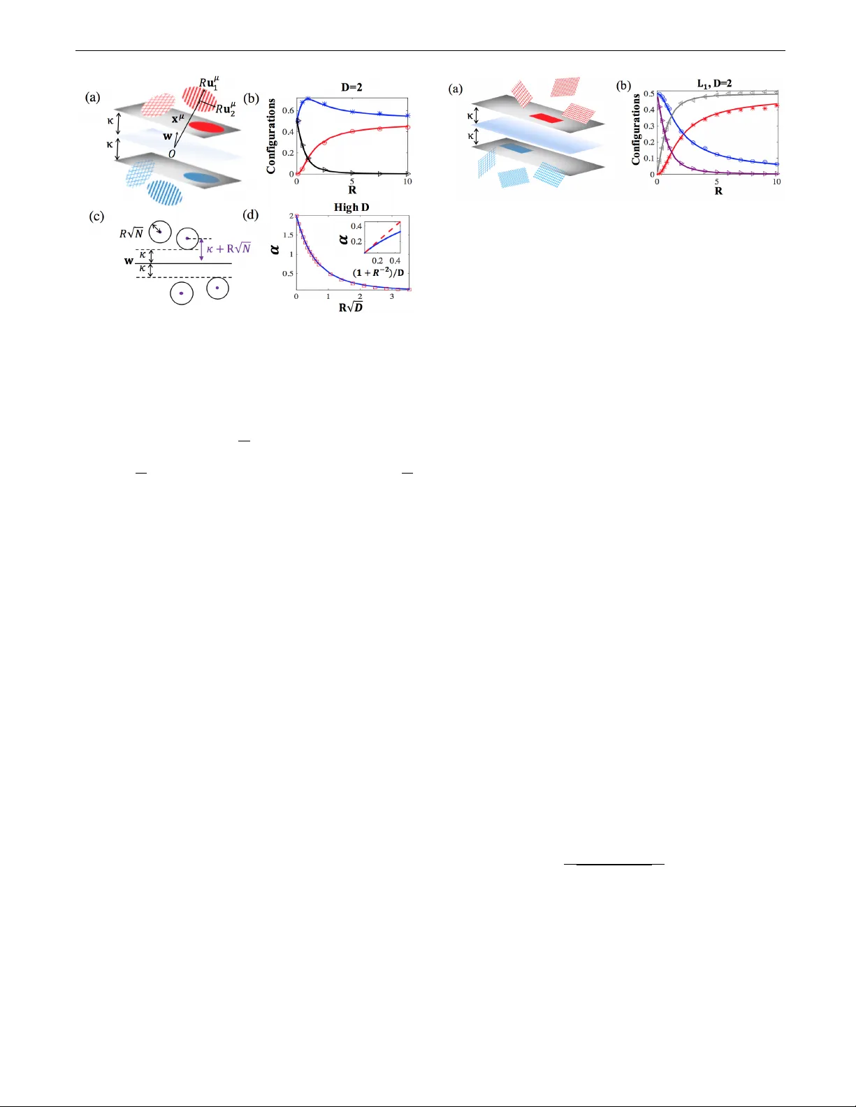
Linear Readout of Ob ject Manifolds SueY eon Ch ung, 1, 2 Daniel D. Lee, 3 and Haim Somp olinsky 2, 4, 5 , ∗ 1 Pr o gr am in Applie d Physics, Scho ol of Engine ering and Applie d Scienc es, Harvar d University, Cambridge, MA 02138, USA 2 Center for Br ain Scienc e, Harvard University, Cambridge, MA 02138, USA 3 Dep artment of Ele ctric al and Systems Engineering, University of Pennsylvania, Philadelphia, P A 19104, USA 4 R ac ah Institute of Physics, Hebr ew University, Jerusalem 91904, Isr ael 5 Edmond and Lily Safr a Center for Br ain Scienc es, Hebr ew University, Jerusalem 91904, Isr ael Ob jects are represented in sensory systems by con tin uous manifolds due to sensitivit y of neu- ronal responses to changes in ph ysical features such as location, orientation, and in tensity . What mak es certain sensory representations better suited for inv ariant decoding of ob jects b y downstream net works? W e presen t a theory that c haracterizes the ability of a linear readout netw ork, the p er- ceptron, to classify ob jects from v ariable neural resp onses. W e show how the readout p erceptron capacit y dep ends on the dimensionality , size, and shap e of the ob ject manifolds in its input neural represen tation. P ACS num b ers: 87.18.Sn, 87.19.lt, 87.19.lv High-lev el p erception in the brain inv olves classifying or iden tifying ob jects which are represented b y contin uous manifolds of neuronal states in all stages of sensory hi- erarc hies [1 – 7] Each state in an ob ject manifold corre- sp onds to the vector of firing rates of resp onses to a par- ticular v ariant of ph ysical attributes which do not c hange ob ject’s iden tity , e.g., intensit y , location, scale, and orien- tation. It has b een hypothesized that ob ject iden tit y can b e deco ded from high level representations, but not from lo w lev el ones, by simple do wnstream readout netw orks [1, 2, 6, 8 – 12]. A particularly simple deco der is the p er- ceptron, which p erforms classification by thresholding a linear weigh ted sum of its input activities [13, 14]. How- ev er, it is unclear what mak es certain representations well suited for inv ariant deco ding by simple readouts such as p erceptrons. Similar questions apply to the hierarch y of artificial deep neural netw orks for ob ject recognition [10, 15–18]. Th us, a complete theory of p erception re- quires characterizing the ability of linear readout net- w orks to classify ob jects from v ariable neural resp onses in their upstream la yer. A theoretical understanding of the p erceptron was pio- neered b y Elizab eth Gardner who form ulated it as a sta- tistical mechanics problem and analyzed it using replica theory [19 – 27]. In this w ork, we generalize the statisti- cal mec hanical analysis and establish a theory of linear classification of manifolds syn thesizing statistical and ge- ometric prop erties of high dimensional signals. W e apply the theory to simple classes of manifolds and show how c hanges in the dimensionality , size, and shap e of the ob- ject manifolds affect their readout b y downstream p er- ceptrons. Line se gments: One-dimensional ob ject manifolds arise naturally from v ariation of stimulus in tensit y , such as visual con trast, whic h leads to appro ximate linear mo dulation of the neuronal resp onses of each ob ject. W e mo del these manifolds as line segments and consider classifying P such segmen ts in N dimensions, expressed as { x µ + Rs u µ } , − 1 ≤ s ≤ 1, µ = 1 , ..., P . The N - dimensional v ectors x µ ∈ R N and u µ ∈ R N denote re- sp ectiv ely , the c enters and dir e ctions of the µ -th seg- men t, and the scalar s parameterizes the contin uum of p oin ts along the segment. The parameter R measures the exten t of the segmen ts relative to the distance b etw een the cen ters (Fig. 1). W e seek to partition the different line segments into tw o classes defined by binary lab els y µ = ± 1 . T o classify the segments, a weigh t vector w ∈ R N m ust ob ey y µ w · ( x µ + Rs u µ ) ≥ κ for all µ and s . The parameter κ ≥ 0 is kno wn as the margin; in general, a larger κ indicates that the p erceptron solution will b e more robust to noise and displa y better generalization prop erties [28]. Hence, we are interested in maxim um margin solutions, i.e., weigh t v ectors w that yield the maximum p ossible v alue for κ . Since line segments are conv ex, only the endp oints of each line segmen t need to b e c heck ed, namely min h µ 0 ± Rh µ = h µ 0 − R | h µ | ≥ κ where h µ 0 = || w || − 1 y µ w · x µ are the fields induced by the centers and h µ = || w || − 1 y µ w · u µ are the fields induced b y the line directions. R eplic a the ory: The existence of a w eigh t vector w that can successfully classify the line segments dep ends up on the statistics of the segmen ts. W e consider random line segmen ts where the components of x µ and u µ are i.i.d. Gaussians with zero mean and unit v ariance, and random binary lab els y µ . W e study the thermo dynamic limit where the dimensionality N → ∞ and n um b er of seg- men ts P → ∞ with finite α = P / N and R . F ollo wing Gardner [19] we compute the a verage of log V where V FIG. 1: (a) Linear classification of p oints. (solid) p oints on the margin, (strip ed) internal points. (b) Linear classification of line segments. (solid) lines embedded in the margin, (dot- ted) lines touching the margin, (strip ed) interior lines. (c) Capacit y α = P / N of a net w ork N = 200 as a function of R with margins κ = 0 (red) and κ = 0 . 5 (blue). Theoretical predictions (lines) and n umerical sim ulation (markers, see SM for details) are sho wn. (d) F raction of differen t line configura- tions at capacity with κ = 0. (red) lines in the margin, (blue) lines touching the margin, (black) in ternal lines. is the v olume of the space of p erceptron solutions: V = ˆ k w k 2 = N d N w P Y µ =1 Θ ( h µ 0 − R | h µ | − κ ) . (1) Θ( x ) is the Heaviside step function. According to replica theory , the fields are describ ed as sums of random Gaus- sian fields h µ 0 = t µ 0 + z µ 0 and h µ = t µ + z µ where t 0 and t are quenched comp onents arising from fluctuations in the input vectors x µ and u µ resp ectiv ely , and the z 0 , z fields represen t the v ariability in h µ 0 and h µ resulting from different solutions of w . These fields m ust obey the constraint z 0 + t 0 − R | z + t | ≥ κ. The capacity func- tion α 1 ( κ, R ) (the subscript 1 denotes the dimensional- it y of the manifolds) describes for whic h P / N ratio the p erceptron solution volume shrinks to a unique weigh t v ector. The recipro cal of the capacit y is given by the replica symmetric calculation (details provided in sup- plemen tary materials, SM): α − 1 1 ( κ, R ) =  min z 0 + t 0 − R | z + t |≥ κ 1 2  z 2 0 + z 2   t 0 ,t (2) where the a verage is o ver the Gaussian statistics of t 0 and t . T o compute Eq. (2), three regimes need to b e consid- ered. First, when t 0 is large enough so that t 0 > κ + R | t | , the minimum o ccurs at z 0 = z = 0 which do es not con- tribute to the capacity . In this regime, h µ 0 > κ and h µ > 0 implying that neither of the t wo segment endp oin ts reac h the margin. In the other extreme, when t 0 < κ − R − 1 | t | , the minimum is given b y z 0 = κ − t 0 and z = − | t | , i.e. h µ 0 = κ and h µ = 0 indicating that b oth endp oints of the line segment lie on the margin planes. In the in- termediate regime where κ − R − 1 | t | < t 0 < κ + R | t | , z 0 = κ − t 0 + R | z + t —, i.e., h µ 0 − R | h µ | = κ but h µ 0 > κ , corresp onding to only one of the line segment endp oin ts touc hing the margin. In this regime, the solution is giv en b y minimizing the function ( R | z + t | + κ − t 0 ) 2 + z 2 with resp ect to z . Com bining these contributions, we can write the p erceptron capacity of line segments: α − 1 1 ( κ, R ) = ˆ ∞ −∞ D t ˆ κ + R | t | κ − R − 1 | t | D t 0 ( R | t | + κ − t 0 ) 2 R 2 + 1 + ˆ ∞ −∞ D t ˆ κ − R − 1 | t | −∞ D t 0  ( κ − t 0 ) 2 + t 2  (3) with integrations ov er the Gaussian measure, Dx ≡ 1 √ 2 π e − 1 2 x 2 dx . It is instructive to consider sp ecial lim- its. When R → 0 , Eq. (3) reduces to α 1 ( κ, 0) = α 0 ( κ ) where α 0 ( κ ) is Gardner’s original capacit y result for p er- ceptrons classifying P p oints (the subscript 0 stands for zero-dimensional manifolds) with margin κ 1-(a). In ter- estingly , when R = 1, then α 1 ( κ, 1) = 1 2 α 0 ( κ/ √ 2). This is b ecause when R = 1 there are no statistical correla- tions b etw een the line segment endp oints and the prob- lem b ecomes equiv alent to classifying 2 P random p oints with a v erage norm √ 2 N . Finally , when R → ∞ , the capacity is further reduced: α − 1 1 ( κ, ∞ ) = α − 1 0 ( κ ) + 1. This is because when R is large, the segments b ecome unbounded lines. In this case, the only solution is for w to b e orthogonal to all P line di- rections. The problem is then equiv alent to classifying P cen ter p oints in the N − P null space of the line directions, so that at capacit y P = α 0 ( κ )( N − P ). W e see this most simply at zero margin, κ = 0. In this case, Eq. (3) reduces to a simple analytic expression for the capacity: α − 1 1 (0 , R ) = 1 2 + 2 π arctan R (SM). The capacit y is seen to decrease from α 1 (0 , R = 0) = 2 to α 1 (0 , R = 1) = 1 and α 1 (0 , R = ∞ ) = 2 3 for un b ounded lines. W e ha v e also calculated analytically the distribu- tion of the cen ter and direction fields h µ 0 and h µ [29]. The distribution consists of three contributions, corresp ond- ing to the regimes that determine the capacity . One com- p onen t corresp onds to line segmen ts fully embedded in these planes. The fraction of these manifolds is simply the v olume of phase space of t and t 0 in the last term of Eq. (3). Another fraction, given by the volume of phase space in the first integral of (3) corresp onds to line segmen ts touching the margin planes at only one end- p oin t. The remainder of the manifolds are those interior to the margin planes. Fig. 1 shows that our theoretical calculations corresp ond nicely with our numerical simu- lations for the p e rceptron capacity of line segments, ev en with mo dest input dimensionality N = 200. Note that 2 as R → ∞ , half of the manifolds lie in the plane while half only touc h it; how ever, the angles betw een these seg- men ts and the margin planes approach zero in this limit. As R → 0 , half of the p oints lie in the plane [29]. D -dimensional b al ls: Higher dimensional manifolds arise from multiple sources of v ariability and their nonlin- ear effects on the neural resp onses. An example is v ary- ing stimulus orientation, resulting in t wo-dimensional ob- ject manifolds under the cosine tuning function (Fig. 2(a)). Linear classification of these manifolds dep ends only upon the prop erties of their conv ex hulls [30]. W e consider simple conv ex hull geometries as D -dimensional balls embedded in N -dimensions: n x µ + R P D i =1 s i u µ i o , so that the µ -th manifold is centered at the vector x µ ∈ R N and its exten t is described by a set of D basis v ectors  u µ i ∈ R N , i = 1 , ..., D  . The p oints in each manifold are parameterized by the D -dimensional v ector ~ s ∈ R D whose Euclidean norm is constrained by: k ~ s k ≤ 1 and the radius of the balls are quantified by R . Statistically , all comp onents of x µ and u µ i are i.i.d. Gaus- sian random v ariables with zero mean and unit v ariance. W e define h µ 0 = N − 1 / 2 y µ w · x µ as the field induced by the manifold cen ters and h µ i = N − 1 / 2 y µ w · u µ i as the D fields induced by each of the basis vectors and with normaliza- tion k w k = √ N . T o classify all the p oints on the mani- folds correctly with margin κ , w ∈ R N m ust satisfy the inequalit y h µ 0 − R || ~ h µ || ≥ κ where || ~ h µ || is the Euclidean norm of the D -dimensional vector ~ h µ whose comp onents are h µ i . This corresp onds to the requirement that the field induced by the points on the µ -th manifold with the smallest pro jection on w b e larger than the margin κ . W e solv e the replica theory in the limit of N , P → ∞ with finite α = P / N , D , and R . The fields for each of the manifolds can b e written as sums of Gaussian quenc hed and entropic comp onents,  t 0 ∈ R , ~ t ∈ R D  and  z 0 ∈ R , ~ z ∈ R D  , resp ectively . The capacity for D -dimensional manifolds is given b y the replica symmet- ric calculation (SM): α − 1 D ( κ, R ) = * min t 0 + z 0 − R k ~ t + ~ z k >κ 1 2 h z 2 0 + k ~ z k 2 i + t 0 , ~ t . (4) The capacity calculation can b e partitioned into three regimes. F or large t 0 > κ + Rt , where t =   ~ t   , z 0 = 0 and ~ z = 0 corresponding to manifolds which lie interior to the margin planes of the p erceptron. On the other hand, when t 0 < κ − R − 1 t , the minimum is obtained at z 0 = κ − t 0 and ~ z = − ~ t corresp onding to manifolds whic h are fully em b edded in the margin planes. Finally , in the intermediate regime, when κ − R − 1 t < t 0 < κ + R t , z 0 = R   ~ t + ~ z   − t 0 + κ but ~ z 6 = − ~ t indicating that these manifolds only touc h the margin plane. Decomposing the capacity ov er these regimes and integrating out the angular comp onents, the capacity of the p erceptron can b e written as: α − 1 D ( κ, R ) = ˆ ∞ 0 dt χ D ( t ) ˆ κ + Rt κ − 1 R t D t 0 ( Rt + κ − t 0 ) 2 R 2 + 1 + ˆ ∞ 0 dt χ D ( t ) ˆ κ − 1 R t −∞ D t 0 h ( κ − t 0 ) 2 + t 2 i (5) where χ D ( t ) = 2 1 − D 2 Γ( D 2 ) t D − 1 e − 1 2 t 2 is the D- Dimensional Chi probabilit y densit y function. F or large R → ∞ , Eq. (5) reduces to: α − 1 D ( κ, ∞ ) = α − 1 0 ( κ ) + D which indicates that w must b e in the null space of the P D basis v ectors { u µ i } in this limit. This case is equiv alent to the classification of P p oin ts (the pro jections of the manifold centers) b y a p erceptron in the N − P D dimensional null space. T o prob e the fields, we consider the joint distribution of the field induced by the cen ter, h 0 , and the norm of the fields induced by the manifold directions, h ≡    ~ h    . There are three contributions. The first term corre- sp onds to h 0 − R h > κ , i.e. balls that lie interior to the p erceptron margin planes; the second comp onent corre- sp onds to h 0 − Rh = κ but h > 0, i.e. balls that touch the margin planes; and the third con tribution represents the fraction of balls ob eying h 0 = κ and h = 0, i.e. balls fully embedded in the margin. The dep endence of these con tributions on R for D = 2 is shown in Fig. 2(b). In- terestingly , when κ = 0 , the case of R = 1 is particularly simple for all D . The capacit y is α D = 2 / ( D + 1) ; in addition, the fraction of em b edded and interior balls are equal and the fraction of touc hing balls ha ve a maxim um, see Fig. 2(b) and SM. In a n um b er of realistic problems, the dimensionality D of the ob ject m anifolds could be quite large. Hence, w e ana- lyze the limit D  1. In this situation, for the capacit y to remain finite, R has to b e small, scaling as R ∝ D − 1 2 , and the capacit y is α D ( κ, R ) ≈ α 0 ( κ + R √ D ). In other words, the problem of separating P high dimensional balls with margin κ is equiv alent to separating P p oints but with a margin κ + R √ D . This is b ecause when the distance of the closest p oint on the D -dimensional ball to the mar- gin plane is κ , the distance of the center is κ + R √ D (see Fig. 2). When R is larger, the capacity v anishes as α D (0 , R ) ≈  1 + R − 2  /D . When D is large, making w orthogonal to a significant fraction of high dimensional manifolds incurs a prohibitive loss in the effectiv e dimen- sionalit y . Hence, in this limit, the fraction of manifolds that lie in the margin plane is zero. Interestingly , when R is sufficien tly large, R ∝ √ D , it becomes adv antageous for w to b e orthogonal to a finite fraction of the mani- folds. L p b al ls: T o study the effect of changing the geomet- rical shap e of the manifolds, we replace the Euclidean norm constraint on the manifold b oundary by a con- strain t on their L p norm. Sp ecfically , we consider D - 3 FIG. 2: Random D -dimensional balls: (a) Linear classifica- tion of D = 2 balls. (b) F raction of 2- D ball configurations as a function of R at capacity with κ = 0, comparing the- ory (lines) with simulations (markers). (red) balls embedded in the plane, (blue) balls touching the plane, (black) interior balls. (c) Linear classification of balls with D = N at margin κ (black circles) is equiv alent to p oint classification of centers with effective margin κ + R √ N (purple p oints). (d) Capacity α = P / N for κ = 0 for large D = 50 and R ∝ D − 1 / 2 as a func- tion of R √ D . (blue solid) α D (0 , R ) compared with α 0 ( R √ D ) (red square). (Inset) Capacity α at κ = 0 for 0 . 35 ≤ R ≤ 20 and D = 20: (blue) theoretical α compared with approximate form (1 + R − 2 ) /D (red dashed). dimensional manifolds n x µ + R P D i =1 s i u µ i o where the D dimensional vector ~ s parameterizing p oints on the man- ifolds is constrained: k ~ s k p ≤ 1. F or 1 < p < ∞ , these L p manifolds are smooth and conv ex. Their linear classifica- tion by a vector w is determined by the field constraints h µ 0 − R || ~ h µ || q ≥ κ where, as b efore, h µ 0 are the fields in- duced by the cen ters, and || ~ h µ || q , q = p/ ( p − 1), are the L q dual norms of the D -dimensional fields induced by u µ i (SM). The resultant solutions are qualitatively similar to what w e observed with L 2 ball manifolds. Ho w ever, when p ≤ 1, the conv ex hull of the mani- fold b ecomes faceted, consisting of vertices, flat edges and faces. F or these geometries, the constraints on the fields asso ciated with a solution vector w b ecomes: h µ 0 − R max i | h µ i | ≥ κ for all p < 1 . W e ha v e solved in detail the case of D = 2 (SM). There are four manifold classes: interior; touching the margin plane at a single v ertex p oint; a flat side embedded in the margin; and fully em b edded. The fractions of these classes are sho wn in Fig. 3. Discussion: W e hav e extended Gardner’s theory of the linear classification of isolated p oints to the classification of contin uous manifolds. Our analysis shows ho w linear separabilit y of the manifolds dep ends intimately up on the dimensionalit y , size and shap e of the conv ex hulls of the manifolds. Some or all of these properties are exp ected to FIG. 3: L 1 balls: (a) Linear classification of 2- D L 1 balls. (b) F raction of manifold configurations as a function of radius R at capacit y with κ = 0 comparing theory (lines) to simulations (mark ers). (red) en tire manifold em b edded, (blue) manifold touc hing margin at a single vertex, (gra y) manifold touching with tw o corners (one side), (purple) interior manifold. differ at different stages in the sensory hierarch y . Thus, our theory enables systematic analysis of the degree to whic h this reformatting enhances the capacity for ob ject classification at the higher stages of the hierarch y . W e fo cused here on the classification of fully observ ed manifolds and hav e not addressed the problem of general- ization from finite input sampling of the manifolds. Nev- ertheless, our results ab out the prop erties of maximum margin solutions can b e readily utilized to estimate gen- eralization from finite samples. The curren t theory can b e extended in sev eral imp ortant wa ys. Additional geo- metric features can b e incorporated, such as non-uniform radii for the manifolds as well as heteogeneous mixtures of manifolds. The influence of correlations in the struc- ture of the manifolds as w ell as the effect of sparse la- b els can also b e considered. The presen t w ork lays the groundw ork for a computational theory of neuronal pro- cessing of ob jects, providing quantitativ e measures for assessing the prop erties of representations in biological and artificial neural net works. Helpful discussions with Remi Monasson and Uri Cohen are ackno wledged. The work is partially supp orted by the Gatsb y Charitable F oundation, the Swartz F oundation, the Simons F oundation (SCGB Grant No. 325207), the NIH, and the Human F rontier Science Program (Pro ject R GP0015/2013). D. Lee also ac kno wledges the supp ort of the US National Science F oundation, Army Researc h Lab oratory , Office of Nav al Research, Air F orce Office of Scien tific Researc h, and Department of T ransp ortation. ∗ Corresp ondence (haim@fiz.h uji.ac.il) [1] J. J. DiCarlo and D. D. Cox, T rends in Cognitive Sciences 11, 333 (2007). [2] M. P agan, L. S. Urban, M. P . W ohl, and N. C. Rust, Nature Neuroscience 16, 1132 (2013). [3] A. Alemi-Neissi, F. B. Rosselli, and D. Zo ccolan, The Journal of Neuroscience 33, 5939 (2013). [4] J. K. Bizley and Y. E. Cohen, Nature Reviews Neuro- 4 science 14, 693 (2013). [5] E. M. Mey ers, M. Borzello, W. A. F reiw ald, and D. Tsao, The Journal of Neuroscience 35, 7069 (2015). [6] R. F. Sch w arzlose, J. D. Swisher, S. Dang, and N. Kan- wisher, Pro ceedings of the National Academy of Sciences 105, 4447 (2008). [7] J. A. Gottfried, Nature Reviews Neuroscience 11, 628 (2010). [8] C. P . Hung, G. Kreiman, T. Poggio, and J. J. DiCarlo, Science 310, 863 (2005). [9] W. A. F reiw ald and D. Y. Tsao, Science 330, 845 (2010). [10] C. F. Cadieu, H. Hong, D. L. Y amins, N. Pinto, D. Ardila, E. A. Solomon, N. J. Ma ja j, and J. J. Di- Carlo, PLoS Comput Biol 10, e1003963 (2014). [11] E. Kobatak e and K. T anak a, Journal of neurophysiology 71, 856 (1994). [12] N. C. Rust and J. J. DiCarlo, The Journal of Neuro- science 30, 12978 (2010). [13] M. L. Minsky and S. A. P ap ert, Perceptrons - Expanded Edition: An Introduction to Computational Geometry (MIT press Boston, MA:, 1987). [14] E. Gardner, Europhysics Letters 4, 481 (1987). [15] T. Serre, L. W olf, and T. Poggio, in IEEE Conference on Computer Vision and Pattern Recognition, CVPR (IEEE, 2005), vol. 2, pp. 994–1000. [16] I. Go o dfellow, H. Lee, Q. V. Le, A. Saxe, and A. Y. Ng, in Adv ances in Neural Information Pro cessing Systems (2009), pp. 646–654. [17] M. A. Ranzato, F. J. Huang, Y.-L. Boureau, and Y. Le- Cun, in IEEE Conference on Computer Vision and Pat- tern Recognition, CVPR (IEEE, 2007), pp. 1–8. [18] Y. Bengio, F oundations and T rends in Machine Learning 2, 1 (2009). [19] E. Gardner, Journal of physics A: Mathematical and General 21, 257 (1988). [20] A. Engel, C. V an den Bro eck, and C. Bro eck, Statisti- cal Mechanics of Learning (Cambridge Universit y Press, 2001). [21] M. Adv ani, S. Lahiri, and S. Ganguli, Journal of Statis- tical Mechanics: Theory and Exp eriment 2013, P03014 (2013). [22] N. Brunel, V. Hakim, P . Isop e, J.-P . Nadal, and B. Bar- b our, Neuron 43, 745 (2004). [23] R. Rubin, R. Monasson, and H. Sompolinsky , Physical Review Letters 105, 218102 (2010). [24] H. Somp olinsky , N. Tishb y , and H. S. Seung, Physical Review Letters 65, 1683 (1990). [25] M. Opp er and D. Haussler, Physical Review Letters 66, 2677 (1991). [26] D. J. Amit, K. W ong, and C. Campb ell, Journal of Ph ysics A: Mathematical and General 22, 2039 (1989). [27] R. Monasson, Journal of Physics A: Mathematical and General 25, 3701 (1992). [28] V. V apnik, Statistical Learning Theory , v ol. 1 (Wiley New Y ork, 1998). [29] L. F. Abb ott and T. B. Kepler, Journal of Physics A: Mathematical and General 22, 2031 (1989). [30] M. De Berg, M. V an Kreveld, M. Ov ermars, and O. C. Sc hw arzkopf, Computational geometry (Springer, 2000). 5