Relaxation of the EM Algorithm via Quantum Annealing

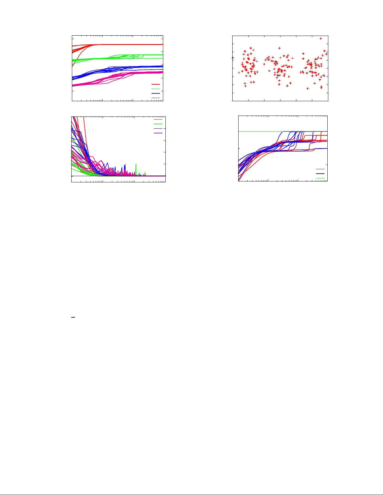
Relaxation of the EM Algorithm via Quantum A nnealing* Hideyuki Miyahara a nd Koji Tsumura Abstract — The EM algorithm is a nov el numerical method to obtain maximum likelihood estimates and is often used f or practical calculations. Howe ve r , many of maximum likelihood estimation pr oblems a re noncon vex , and it is known that the EM algorithm fails to give th e o ptimal estimate by bein g trapped by local optima. In order to d eal with this di ffi culty , we propose a deterministic quantum a nnealing EM algorithm by introducing the mathematica l mechanism of quantum fluctuations into the conv entional EM algorithm because quantum fluctu ations induce the tunnel e ff ect and ar e expected to r elax the di ffi culty of nonconv ex optimization pr oblems in the max imum likelihood estimation problems. W e sh ow a theorem that guarantees its con ver gence and giv e n umerical experiments to verify its e ffi ciency . I. I ntr oduction Many o f pr actical p roblem s in engineering or the prin- ciples to explain the phenomena of nature a re r educed into non conv ex optimization ; ho wev er , the r esearch activity for n onconve x optimizatio n is limited compa red to that on conv ex optimiza tion becau se it is fundam entally di ffi cult to solve or analyze the pro blem in a sophisticated way . In ord er to solve this di ffi cu lty of n onconve x o ptimization , motiv ated by the physical process of ann ealing, Kirk patrick et al. [1], [2] prop osed simulated annea ling (SA). SA h as attracted much attention in many field s because SA has the following two rema rkable pro perties. The first one is that SA can be a pplied to any nonconve x prob lems. The second o ne is that its glob al co n vergence in some sense is guaranteed b y Geman and Geman [3]. After that, quantu m an nealing (QA) was proposed by Apolloni et al. [4]. In QA, the mathematical mechanism of q uantum fluctuations is intro duced, a nd it has been reported that QA can reduce com putation al co sts in many di ffi cult prob lems [5], [6], [7 ], [8], [9], [10], [11], [12], [1 3], [14]. Desp ite the success of SA and QA , the ir computatio nal costs are still huge , because the Monte Carlo method is used in most of their implementatio ns and it requires m uch computation al costs fo r c onv ergence. On th e o ther h and, in or der to solve the non conv ex problem in data clu stering, Rose et al. [15 ], [16] propo sed a deterministic simulated ann ealing approach , an d it attracted interest in both o f phy sics and eng ineering . This is becau se it can relax the problem of local optima with almost the same numerical cost wh ich is req uired f or a c onv entional appr oach. As a genera lization of [15], [16], Ueda and Naka no [17 ] propo sed a deterministic simulated a nnealing EM algor ithm *This work was supported in part by Grant-in- Aid for Scientific Researc h (B) (25289127), Japan Society for the Promotion of S cienc e. H. Miyahara and K. Tsumura are with the Department of In- formation Physics and Computing, the G raduate School of Infor- mation Science and T e chnolog y , The Univ ersity of T ok yo, Japan hideyuki miyahara@i pc.i.u-tok yo.ac.jp T ABLE I : Classi fication of the alg orithms Fluctua tions Anneali ng 1 D AEM 2 Thermal Kirkpatri ck et al. [1], [2] 3 Ueda & Nakano [17] 4 Quantum Apolloni et al. [4] 5 This work 6 (DSAEM). T he EM algo rithm (E M), wh ich was originally propo sed by Demp ster et al. [18], is a g eneric app roach to compute the max imum likelihood estimates, but it is k nown that it su ff ers from the proble m of local optima. DSAEM was reported to be m ore e ff ecti ve than EM when EM is likely to be trapped b y local optima; h owe ver the pr oblem of loc al optima is still fun damental in optimization and it ha s b een tackled via many approach es. From the above discu ssions, this p aper p resents a de- terministic quan tum annealing EM alg orithm (DQAEM) by intro ducing the math ematical mechan ism of quantu m fluctuations to EM. In DQAEM, qu antum fluctuations are introdu ced becau se it may induc e the tun nel e ff ect and it is con sidered to be e ff ecti ve to solve non conv ex o pti- mization p roblem s. Howe ver , it is known to be di ffi cult to ev aluate function s with q uantum fluc tuations, an d our key idea to compr omise this di ffi cu lty is to ap ply the Feynman path inte gral for mulation to DQAEM. In this paper , after explaining EM , we giv e the formu lation of DQAEM and how it is a pprox imated through th e Fe ynman path integral formu lation. Th en, we present a theorem th at en sures the monoto nicity of its cost function, called the “fr ee e nergy , ” during the iterations in the algo rithm. Th at is, DQAE M is g uaranteed to con ver ge to the global op timum or local optima. At the end of this paper, in o rder to show the e ffi ciency of DQAEM, we app ly DQAEM and EM to a parameter estimation problem and illu strate that DQAEM is superio r to EM . W e sum marize the algo rithms mention ed above in T a ble I for conv enience. This paper is organized as follows . In Sec. II, E M proposed by Dempster et a l. [18] is reviewed for p reparatio n of DQAEM. In Sec. II I, we prop ose DQAEM and giv e a theorem on its convergence. I n Sec. IV, we show nume rical simulations to verify the theor em and the e ffi ciency of DQAEM c ompared with EM. Finally , in Sec. V, we give the conclusion of this paper . II. R eview o f the E M algorithm ( EM) In this section , we review EM, which was propo sed by Demp ster et al. [18] for the preparation of in troduc- ing DQAEM. In this paper, Y obs = { y (1) , y (2) , . . . , y ( N ) } and { x (1) , x (2) , . . . , x ( N ) } denote an observable d ata set and an unobser vable da ta set, respectively . Moreover , we assume that e ach data point y ( i ) ( i = 1 , 2 , . . . , N ) is indep endent and identically d istributed. T hen, at first, we define max imum likelihood estimatio n ( MLE). In MLE, the cost f unction, which is called the log likelihood function, is given by L ( Y obs ; θ ) = N X i = 1 log p ( y ( i ) ; θ ) = N X i = 1 log Z d x ( i ) p ( y ( i ) , x ( i ) ; θ ) , (1) where p ( y ; θ ) a nd p ( y , x ; θ ) are prob ability density functions for incomplete data and co mplete data, r espectively , and θ is a param eter . Then the p arameter θ is determin ed by the maximization o f L ( Y obs ; θ ) with resp ect to θ . Note that in the case that p ( y ; θ ) belong s to the exponential family , the maximization can be easily attained. In m ost prac tical cases, h owe ver , p ( y ; θ ) do es not b elong to th e exponential family , and th en the maxim ization of L ( Y obs ; θ ) is di ffi cu lt to compute. EM was proposed as an iterativ e approach to calculate the max imum likelihood esti- mates in these cases, and th en the maximizatio n of L ( Y obs ; θ ) is replace d by its lower bound called the Q functio n. W e then derive the Q function as follows: L ( Y obs ; θ ) ≥ Q ( θ ; θ ′ ) − N X i = 1 Z d x ( i ) p ( x ( i ) | y ( i ) ; θ ′ ) log p ( x ( i ) | y ( i ) ; θ ′ ) , (2) Q ( θ ; θ ′ ) = N X i = 1 Z d x ( i ) p ( x ( i ) | y ( i ) ; θ ′ ) log p ( y ( i ) , x ( i ) ; θ ) , (3) where the par ameter θ ′ is an arbitrar y parameter and Jensen’ s inequality is u sed to d erive the inequality . Note that th e Q function includes a conditional p robab ility density function p ( x | y ; θ ), a nd it is comp uted with Bayes’ rule as p ( x ( i ) | y ( i ) ; θ ′ ) = p ( y ( i ) , x ( i ) ; θ ′ ) R d x p ( y ( i ) , x ; θ ′ ) , (4) for i = 1 , 2 , . . . , N . Then, th e parameter θ ( t ) is updated by θ ′ = θ ( t ) and θ ( t + 1) = arg max θ Q ( θ ; θ ( t ) ) . (5) The calculation of (3) is called the E step and that of (5) is called the M step, an d they are iterated until terminatio n condition s are satisfied. W e summar ize EM in T able 1 . EM is widely used becau se it h as two remar kable prop- erties as follows. Th e fir st one is that it can be applied to mixture mod els, which o ften appear in practical applications, and it g iv es better perfo rmance than conv e ntional metho ds in ma ny cases. The second one is th at the log likelihood function mo noton ically increase via its iteration s, and th is implies that it is stab le through iteration s. Howev e r it is also known to be trapp ed by lo cal optima and its pe rforma nce heavily d epends on an initial estimated parameter, and thus this problem is a moti vation of o ur study . Algorithm 1 The EM algorith m (EM) 1: initialize θ (0) and set t ← 0 2: while co n vergence criterion is satisfied do 3: calculate p ( x ( i ) | y ( i ) ; θ ( t ) ) for i ( i = 1 , 2 , . . . , N ) with (4) (E step) 4: calculate θ ( t + 1) = arg max θ Q ( θ ; θ ( t ) ) wher e Q ( θ ; θ ( t ) ) is (3) (M step) 5: end while III. D eterministic qu ant um anneali ng EM algorithm (DQAEM) Here, we der iv e DQAEM, which is th e main concep t of this paper, by introduc ing the mechanism of quan tum fluc- tuations into EM. W e then gi ve a theorem which guaran tees its con vergen ce. A. Derivation First, we define the cost function, wh ich is called the free energy , as F β, Γ ( θ ) = − 1 β log Z β, Γ ( θ ) , (6) where Z β, Γ ( θ ) = N Y i = 1 Z ( i ) β, Γ ( θ ) , (7) Z ( i ) β, Γ ( θ ) = Z d x ( i ) h x ( i ) | p Γ ( y ( i ) , ˆ x ; θ ) β | x ( i ) i , p Γ ( y ( i ) , ˆ x ; θ ) = exp {− ( H ( y ( i ) , ˆ x ; θ ) + H kin ) } ( i = 1 , 2 , . . . , N ) , (8) ˆ x represents a position operator, H ( y ( i ) , ˆ x ; θ ) = − log p ( y ( i ) , ˆ x ; θ ), and H kin is a fu nction of a momentum operator ˆ π . Th is momen tum operator ˆ π satisfies the commutatio n relation [ ˆ x , ˆ π ] = i ¯ h . In th is pa per, we consider the form H kin = ˆ π 2 / 2 µ to simplify later calculations. From the definitio n of the free energy (6) an d the log likelihood function (1), they hold the following identity , F β = 1 , Γ= 0 ( θ ) = −L ( Y obs ; θ ) . (9) W e then in terpret th e n egati ve fr ee energy as an extension of the log likelihood f unction . Second, in order to formu late DQAEM, we divide the free energy (6) into two parts as fo llows, F β, Γ ( θ ) = U β, Γ ( θ ; θ ′ ) − 1 β S β, Γ ( θ ; θ ′ ) , U β, Γ ( θ ; θ ′ ) = N X i = 1 Z d x ( i ) D x ( i )     h − f β, Γ ( ˆ x ( i ) | y ( i ) ; θ ′ ) log p Γ ( y ( i ) , ˆ x ( i ) ; θ ) i     x ( i ) E , (10) S β, Γ ( θ ; θ ′ ) = N X i = 1 Z d x ( i ) D x ( i )     h − f β, Γ ( ˆ x ( i ) | y ( i ) ; θ ′ ) log f β, Γ ( ˆ x ( i ) | y ( i ) , θ ) i     x ( i ) E , (11) with the operator of the per turbed conditional probability density function, f β, Γ ( ˆ x ( i ) | y ( i ) ; θ ) = p Γ ( y ( i ) , ˆ x ( i ) ; θ ) β Z ( i ) β, Γ ( θ ) . (12) The fun ction U β, Γ ( θ, θ ′ ) is an extension of th e Q functio n (3), and satisfies the identity U β = 1 , Γ= 0 ( θ, θ ′ ) = − Q ( θ , θ ′ ) . As the Q function is op timized instead of the log likelihoo d function in EM, the function U β, Γ ( θ, θ ′ ) is o ptimized in DQAEM. In some s pecial case, the calculations of the free energy (6) and the energy (10) can be perf ormed analytically; h owe ver those are di ffi cult in g eneral when an assumed mo del has a complicated form. W e thus use the Feynman’ s path integral formu la [19], [20], [21], [22] to simplify the calcu lation of U β, Γ as U β, Γ ( θ ; θ ′ ) ≈ N X i = 1 Z M Y j = 1 d x ( i ) j " − 1 M f β, Γ ( { x ( i ) j }| y ( i ) ; θ ′ ) M X j = 1 log p ( y ( i ) , x ( i ) j ; θ ) # + const ., (13) with f β, Γ ( { x ( i ) j }| y ( i ) ; θ ′ ) = 1 Z ( i ) β, Γ ( θ ′ ) M 2 πβ Γ ! M / 2 exp M X j = 1 β M log p ( y ( i ) , x ( i ) j ; θ ′ ) − M X j = 1 M 2 β Γ ( x ( i ) j − x ( i ) j − 1 ) 2 ! , (1 4) where M is th e number of b eads, { x ( i ) j } represents { x ( i ) j } M j = 1 and the periodic bo undar y con ditions x ( i ) 0 = x ( i ) M for each i ( i = 1 , 2 , . . . , N ) are satisfied. The upd ating equation fo r th e parameter θ is ther efore g iv en by θ ( t + 1) = arg min θ U β, Γ ( θ ; θ ( t ) ) . W e put the above calculations to an algorithm as DQAEM, which includes two steps called the E step and th e M step. In the E step of DQAEM, f β, Γ ( { x ( i ) j }| y ( i ) ; θ ( t ) ) in (14) is computed , and in the M step of DQAEM , the pa rameter θ ( t ) is updated by the minimization of (13). Finally , we summarize the algorithm in T able 2. B. Con v er gence th eor e m In general, stability of an algorith m is not obvio us, and here we give a theorem that guaran tees the stability of DQAEM th rough iterations as follows. Theor em 1: Let the parameter θ ( t + 1) be given by θ ( t + 1) = arg min θ U β, Γ ( θ ; θ ( t ) ). Then the ine quality F β, Γ ( θ ( t + 1) ) ≤ F β, Γ ( θ ( t ) ) holds. The equality holds Algorithm 2 Determ inistic quantum ann ealing E M algorithm (DQAEM) 1: set β ← β init (0 < β init ≤ 1 ) 2: set Γ ← Γ init (0 ≤ Γ init ) 3: initialize θ (0) and set t ← 0 4: while co n vergence criteria is satisfied do 5: calculate f β, Γ ( { x ( i ) j }| y ( i ) ; θ ( t ) ) for i ( i = 1 , 2 , . . . , N ) with (14) (E step) 6: calculate θ ( t + 1) = arg m in θ U β, Γ ( θ ; θ ( t ) ) with (13) (M step) 7: increase β and decrease Γ 8: end while if and only if U β, Γ ( θ ( t + 1) ; θ ( t ) ) = U β, Γ ( θ ( t ) ; θ ( t ) ) and S β, Γ ( θ ( t + 1) ; θ ( t ) ) = S β, Γ ( θ ( t ) ; θ ( t ) ) are satisfied. By this th eorem, we c an co nclude that DQAEM is guar an- teed to con verge to the global optimum or a local optimum. It is k nown that the mono tonicity of th e log likelihood f unction in EM an d some ma thematical features of EM are proved by Dempster et al. [18] and W u [23], and this th eorem clarifies that the similar mono tonicity also holds in DQAEM. IV . N umerical simula tions In th is section, we give nu merical simulations to show the e ffi ciency o f DQAEM in comparison with EM. At, first we begin with the defin ition of the pro blem that we co nsider in this section . Next, we giv e the numerical simulation s which support the theo rem shown in the previous section. Finally , we co mpare DQA EM and EM b y app lying th em to the problem and discu ss th e e ffi c iency of DQAEM. A. Mathematical fo rmulation W e ado pt the mixtur e of factor analysis (MF A) [24], [ 25] as th e prob lem to wh ich DQ AEM and EM are app lied in this section. MF A is a mo del to analyze hid den factors in a gi ven data set, and is a ty pical no nconve x op timization problem if the numbe r of factors is larger th an 1. Accord ingly , EM is often applied to MF A for p ractical calculations. MF A can be considered to assume following two steps to generate data. In th e first step, a factor is iden tified by an index parame ter w ∈ { 1 , 2 , . . . , m } , wh ich is generated with a probab ility P ( w ), and an uno bservable state x is g enerated with a probab ility density fun ction p ( x ). In the second step, the o bservable v ariable y is gen erated by the transfor mation of x de pending on w and an ad ditive noise. This transfor- mation is represented by p ( y | x , w ; θ ). The probability d ensity function for y is then given by p ( y ; θ ) = m X w = 1 Z d x p ( y , x , w ; θ ) , (15) p ( y , x , w ; θ ) = p ( y | x , w ; θ ) p ( x ) P ( w ) , (16) where P ( w = i ) = π i , p ( x ) = N (0 , I ), p ( y | x , w = i ; θ ) = N ( µ i + Λ i x , Φ ), and m is the assumed n umber of facto rs in MF A. For simplicity , we d enote { π i , µ i , Λ i , Φ } m i = 1 by θ . (a) -1000 -800 -600 -400 -200 1 10 100 1000 − F β , Γ ( θ ( t ) ) Iterations ( t ) m = 1 m = 3 m = 7 m = 10 (b) 0 10 20 30 40 50 1 10 100 1000 − F β , Γ ( θ ( t +1) ) + F β , Γ ( θ ( t ) ) Iterations ( t ) m = 1 m = 3 m = 7 m = 10 Fig. 1: Number of iteratio ns vs (a) negati ve free energy and (b) di ff e rence o f negative free energies in each step for 4 models whose nu mbers of mixtures are m = 1 , 3 , 7 and 10. In DQAEM for MF A, th e Hamilton ian H kin , wh ich rep - resents the kinetic term, is added to the or iginal model of MF A, and then we hav e the following p Γ ( y , ˆ x , w ; θ ) = p ( y | ˆ x , w ; θ ) e − ( H + H kin ) P ( w ) , (17) where H = − log p ( ˆ x ) and H kin = ˆ π 2 / 2 µ ( H kin = − Γ ∂ 2 /∂ x 2 with Γ = ¯ h 2 /µ in x -bases). Supp ose we hav e N data po ints Y obs = { y (1) , y (2) , . . . , y ( N ) } , and then the free energy is given by F β, Γ ( θ ) = N X i = 1 − 1 β log m X w ( i ) = 1 Z d x ( i ) D x ( i )    p Γ ( y ( i ) , ˆ x ( i ) , w ( i ) ; θ ) β    x ( i ) E . (18) In n umerical experime nts, M is set to 128, th e ann ealing parameter Γ , which r epresents the stren gth of q uantum fluctuations, is controlled fro m an in itial value to 0 linearly , and the inv erse tem perature β is fixed at 1. B. Numerical r esults I W e have shown the mon otonicity o f th e free energy ( 6) in DQAEM in Sec. II I-B, a nd here we verify T heorem 1 via numerical experimen ts. In this subsection, we consider 4 models which have 1, 3 ,7 and 10 mixtures, respectively . The transitions of n egati ve f ree energies − F β, Γ ( θ ( t ) ) for these mo dels are shown in Fig. 1(a), and the ch ange of them − F β, Γ ( θ ( t + 1) ) + F β, Γ ( θ ( t ) ) is plotted in Fig. 1(b). By observin g Fig. 1, we can co nfirm that the negativ e free en ergy varies monoto nically in DQAEM. In th e case that m = 1 , this problem is a con vex optimization, and thus w e can see that (a) -8 -4 0 4 8 -1.5 -1 -0.5 0 0.5 1 1.5 Y coordinate X coordinate Data (b) -600 -550 -500 -448.4 -400 1 10 100 1000 L ( y ; θ ( t ) ) an d − F β , Γ ( θ ( t ) ) Iterations ( t ) EM DQAEM Optimal v alue Fig. 2: (a) Da ta set generated by th ree Gaussian functions whose means are ( X , Y ) = ( − 1 , 0), ( 0 , 0) and (1 , 0). (b) Numb er of iteration s (log scale) vs the log likelihood f unctions in EM and the negative free energies in DQAEM. the n egati ve free e nergies co n verge to the unique o ptimal value in Fig. 1( a). C. Numerical results I I This sub section is devoted to the compar ison betwee n DQAEM and EM to show the e ffi ciency of DQAEM. W e deal wi th the d ata sh own in Fig. 2, which are generated by the Gaussian mixture model whose mean s are ( X , Y ) = ( − 1 , 0), (0 , 0) a nd (1 , 0). In Fig. 2(b), th e tran sients of the log likelihood functio ns by EM are p lotted by red lines and those o f the negative free energies by DQAEM are p lotted by blue lines. The green line r epresents the v alue of − 448 . 4 , which correspo nds to the o ptimal estimation in this p roblem. Som e of red lin es and blu e lines co n verge to the value of − 4 48 . 4, and thus DQAEM an d EM gi ve the optimal estimation in these cases. On the othe r h and, some of red lin es and blue lines con verge to lo wer values th an the optimal estimation. Howe ver, th e ratios whether DQAEM and EM gives the optim al estimation are m uch di ff erent. W e perfor med DQAEM and EM 1000 times with th e same initial condi- tions, and the ratios whether DQAEM and EM succee d or fail with the same ran domized initial p arameters are summarized in T able II . Her e, the “su ccess” of DQAEM and E M is defined as that square er rors between the estimated means of th ree Gaussian function s a nd th e true m eans ar e smaller than 0 . 2 times the c ovariances of three Gaussian f unction s. This table shows that D QAEM succeeds with the ratio 90.7% while EM succeeds with the r atio 36. 6%, and that DQAEM T ABLE II: Ratios whether DQAEM a nd E M succeed o r fail for this problem (Th e details o f th e cases labeled by ( ∗ ) and ( ∗∗ ) are discussed in Secs. IV - C.1 (Case I ( ∗ ) ) and IV - C.2 (Case II ( ∗∗ ) ), respectiv ely). DQAEM Success Fail T otal Success 36.3 % ( ∗ ) 3.3 % 36.6 % EM Fail 54.4 % ( ∗∗ ) 9.0 % 63.4 % T otal 90.7 % 9.3 % 100.0 % (a) -600 -550 -500 -448.4 -400 0 200 400 600 800 1000 L ( y ; θ ( t ) ) an d − F ( θ ( t ) ) Iterations ( t ) EM DQAEM Optimal v alue (b) -2 -1.5 -1 -0.5 0 0.5 1 1.5 0 200 400 600 800 1000 Estimated X coordinates of means Iterations ( t ) EM DQAEM T rue value Fig. 3: (a ) Number of iter ations vs th e log likelihood fun c- tions o f E M an d the negati ve free energies o f DQAEM with the initial estimated par ameters with which bo th EM and DQAE M give glob al o ptimums (Case I ( ∗ ) ). Green lin e exhibits th e optim al value. ( b) Numb er of iteratio ns vs th e estimated X coordinates o f m eans of Gaussian functions by EM, and those by DQAE M in Case I ( ∗ ) . Green lines stand for the true values. is su perior to EM. 1) Case I ( ∗ ) : Here we fo cus on the conver gence ra tes of DQAEM an d EM in th e case that bo th of them succ eed in parameter estimation. First, we plot the log likelihood f unction s and the negative free energies in Fig. 3(a) and the estimated X coord inates in Fig. 3(b ). In this case, both the log likelihood functions and the negative fr ee energies co n verge to th e value of − 448 . 4, and the estimated X co ordina tes go to th e n eighbo rs around − 1 . 0, 0 . 0 and 1 . 0. Th ese figures a lso imp ly that DQAEM conv e rges to the optimal estimation faster than EM. W e also show the numb er o f iter ations that are requir ed until DQ AEM an d E M satisfy th e criter ia o f the “success” in T able III. This table tells us that DQAEM is app roxima tely T ABLE I II: Nu mbers o f iter ations that a re required fo r DQAEM an d EM to satisfy the cr iteria o f th e “success. ” DQAEM EM 65.33 times 243.82 times 3.73 tim es faster than EM. 2) Case II ( ∗∗ ) : At the end of th is section, we analyze the behaviors of DQAEM and EM in the case that DQAEM succeeds and E M fails. In Fig. 4(a), the log likelihoo d function s of EM an d th e negati ve free energies of DQAEM are plotted . It is o bserved that while DQA EM gives the value of − 448 . 4, EM gives lower values than that and is trappe d by some local optim a. The estimated X coordinates by EM and DQAEM are shown Figs. 4(b) and ( c), respectively . While the estimated X c oordin ates by DQAEM con verge in the neighb ors around − 1 . 0 , 0 . 0 an d 1 . 0, th e estimated X coordin ates by EM go to di ff erent v alu es. V . C onclusion W e hav e pro posed a dete rministic qu antum annealing EM algor ithm (DQAEM) in this p aper . In DQAEM , the mathematical m echanism of quantum fluctuation s is intro - duced in to EM, and then our pro posed algor ithm is regarded as a quantum version of that by Ueda and Nakano [1 7]. Then we sh ow a the orem on th e mo notonicity of DQAE M mathematically , that is, it guarantees that DQAEM is stable in the algorithm iterations. Th rough numerical experiments, we also confirmed the monotonicity of DQAEM, and then we compared DQAEM and EM . In th e comparison , we observe that DQAEM succeeds in parameter estimates with higher prob ability and faster th an EM. At the end, we mention our future w ork. DQAEM in this paper is fo r models with continuou s latent variables, and then o ne o f our future works is to for mulate DQAEM for models with discrete latent variables, w hich usually appear in various en gineerin g problem s. R eferences [1] S. Kirkpat rick, C. D. Gelat t, and M. P . V ecc hi, “Optimiz ation by simulate d annea ling, ” Science , vol. 220, no. 4598, pp. 671–680, 1983. [Online]. A v ailable: http: // www . science mag.org / conte nt / 220 / 4598 / 671.abstract [2] S. Kirkpatrick, “Optimiza tion by simulat ed anneali ng: Quantita tiv e studies, ” Journal of Statistical P hysics , vol. 34, no. 5-6, pp. 975–986, 1984. [Online]. A va ilabl e: http: // dx.doi.org / 10.1007 / BF0100945 2 [3] S. Geman and D. Geman, “Stochastic rela xation, gibbs distrib utions, and the bayesian restoration of images, ” P attern Analysis and Machine Intell ige nce, IEE E T ransactions on , vol. P AMI-6, no. 6, pp. 721–741, Nov 1984. [4] B. Apollon i, C. Carva lho, and D. de Fal co, “Quantum stochasti c optimizat ion, ” Stochasti c Pr ocesses and their A pplicat ions , vol. 33, no. 2, pp. 233–244, 1989. [Online]. A vaila ble: http: // www . science direct.c om / science / article / pii / 0304414989900409 [5] A. Finnila, M. Gomez, C. Sebenik, C. Stenson, and J. Doll, “Quantum annealing : A ne w m ethod for minimizing multidime nsional functio ns, ” Chemica l Physics Letters , vol. 219, no. 56, pp. 343–348, 1994. [Online]. A v ailab le: http: // www . science direct.c om / science / article / pii / 0009261494001170 [6] T . Kadow aki and H. Nishimori, “Quantum anneali ng in the transverse ising m odel, ” Phys. Rev . E , vol. 58, pp. 5355–5363, No v 1998. [Online]. A vail able: http: // link.aps.org / doi / 10.1103 / PhysRe vE.58.5355 (a) -600 -550 -500 -448.4 -400 0 200 400 600 800 1000 L ( y ; θ ( t ) ) an d − F ( θ ( t ) ) Iterations ( t ) EM DQAEM Optimal v alue (b) -1.5 -1 -0.5 0 0.5 1 1.5 0 200 400 600 800 1000 Estimated X coordinates of means Iterations ( t ) EM T rue value (c) -1.5 -1 -0.5 0 0.5 1 1.5 0 200 400 600 800 1000 Estimated X coordinates of means Iterations ( t ) DQAEM T rue value Fig. 4: (a ) Number of iter ations vs th e log likelihood fun c- tions of EM and th e negati ve fr ee energies of DQAEM with the initial estimated parame ters with which EM f ails and DQAEM succeed s (Case II ( ∗∗ ) ). Green line stand fo r the optimal value. (b ) Numb er of iterations vs the e stimated X coord inates of means of Gau ssian functions by EM in Case II ( ∗∗ ) . Green lines stan d for th e true values. (c) Nu mber of iterations vs the estimated X coordina tes of means of Gaussian functions by DQAEM in Case I I ( ∗∗ ) . Gr een lines stand f or the tr ue values. [7] J. Brooke , D. Bitk o, T . F ., Rosenbaum, and G. Aeppli, “Quantum anneal ing of a disordered magnet, ” Sc ience , vol. 284, no. 5415, pp. 779–781, 1999. [Online]. A v ailable: http: // www . science mag.org / conte nt / 284 / 5415 / 779.abstract [8] D. de Falco and D. T amascelli , “Quantum anneal ing and the s chr ¨ odinger -lange vin-kostin equati on, ” Phys. Rev . A , vol. 79, p. 012315, Jan 2009. [Online]. A va ilable : http: // lin k.aps.org / doi / 10.1103 / PhysRe vA.79.012315 [9] ——, “ An introduct ion to quantum anneali ng, ” RA IR O - Theor etical Informatic s and A pplicat ions , vol. 45, pp. 99–116, 1 2011. [10] A. Das and B. K. Chakrabar ti, “ Colloquium : Quantum anneal ing and analog quantu m computation , ” R ev . Mod. P hys. , vol. 80, pp. 1061–1081, Sep 2008. [Online]. A vai lable: http: // lin k.aps.org / doi / 10.1103 / Re vModPhys.80.1061 [11] E. Farhi, J. Goldstone, S. Gutmann, J. Lapan, A. Lundgren, and D. Preda, “ A quantum adiabatic ev olution algorit hm applied to random instances of an np-complete problem, ” Science , vol. 292, no. 5516, pp. 472–475, 2001. [Online]. A v ailable: http: // www . science mag.org / conte nt / 292 / 5516 / 472.abstract [12] G. E. Santoro, R. Marto ˇ n ´ ak, E. T osatti, and R. Car , “Theory of quantum annealin g of an ising spin glass, ” Science , vol. 295, no. 5564, pp. 2427–2430, 2002. [Online]. A va ilabl e: http: // www . science mag.org / conte nt / 295 / 5564 / 2427.abstract [13] G. E. Santoro and E . T osatti, “Optimizat ion using quantum mechanics: quantum annealin g through adiabati c evo lution, ” J ournal of P hysics A: Mathemat ical and General , vol. 39, no. 36, p. R393, 2006. [14] R. Marto ˇ n ´ ak, G. E. Santoro, and E. T osatti, “Quant um annealing by the pat h-integral monte carlo method: The two-dimension al random ising model, ” Phys. Rev . B , vo l. 66, p. 094203, Sep 2002. [Onl ine]. A vailab le: http: / / link.aps.org / doi / 10.1103 / PhysRe vB.66.094203 [15] K. Rose, E. Gure witz, and G. Fox, “ A deterministic anneal ing approach to clusterin g, ” P attern Recogn ition Letters , vol. 11, no. 9, pp. 589–594, 1990. [Online]. A vaila ble: http: // www . science direct.c om / science / article / pii / 016786559090010Y [16] K. Rose, E. Gure witz, and G. C. Fox, “Statistica l mechanic s and phase transiti ons in clustering , ” Phys. Rev . Lett. , vol. 65, pp. 945–948, Aug 1990. [Online]. A v ailable: http: // lin k.aps.org / doi / 10.1103 / PhysRe vLett.65.945 [17] N. Ueda and R. Nakano, “Determinist ic anneal ing em algorithm, ” Neu- ral Networks , v ol. 11, no. 2, pp. 271–282, 1998. [Online]. A va ilable : http: // www . science direct.c om / science / article / pii / S0893608097001330 [18] A. P . Dempster , N. M. Laird, and D. B. Rubin, “Maximum likel ihood from inco mplete data via the em algorithm, ” JOURN AL OF T HE R OY AL STA TISTICAL SOCIETY , SERIES B , vol. 39, no. 1, pp. 1–38, 1977. [19] R. P . Fe ynman and A. R. Hibbs, Quantu m mec hanics and path inte grati on . McGrawsHil l, 1965. [20] R. P . Feyn man, Statistical Mecha nics: A Set of Lectur es . Benjamin Readin g, 1972 . [21] M. T akahashi and M. Imada, “Monte carlo calc ulatio n of quantum systems, ” Jo urnal of the Physical Society of Japa n , vol. 53, no. 3, pp. 963–974, 1984. [Online]. A vaila ble: http: // dx.doi.or g / 10.1143 / JPSJ.53.963 [22] ——, “Monte carlo calc ulation of quantum systems. ii. higher order correct ion, ” Journal of the Physical Socie ty of Jap an , vol. 53, no. 11, pp. 3765–3769, 1984. [Online ]. A va ilable : http: // dx.doi.or g / 10.1143 / JPSJ.53.3765 [23] C. F . J. Wu, “On the con ver gence propertie s of the em algorit hm, ” Ann. Statist. , vol. 11, no. 1, pp. 95–103, 03 1983. [Online]. A v ailabl e: http: // dx.doi.or g / 10.1214 / aos / 1176346060 [24] Z. Ghahramani, G. E. Hinton, et al. , “The em algorith m for mixtures of facto r analyzers, ” 1996. [25] K. P . Murphy , Machine learning : a pr obabilist ic per spective . MIT press, 2012.