Coordinate Friendly Structures, Algorithms and Applications

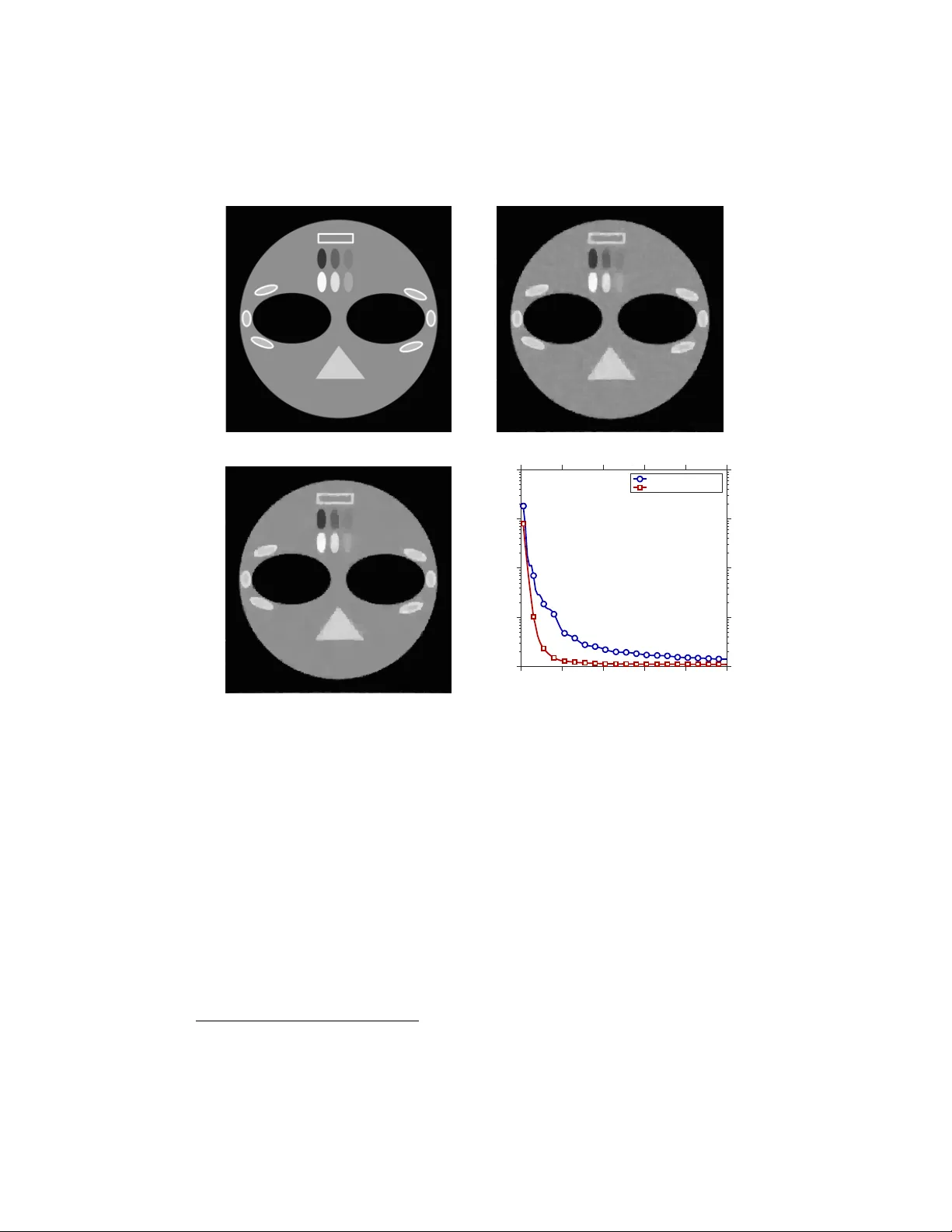
Co ordinate friendly structures, algorithms and applications ∗ Zhimin Peng , Tianyu Wu , Y angy ang Xu , Ming Y an , and W ot ao Yin This pap er fo cuses on c o or dinate up date metho ds , which are useful for solving problems in volving large or high-dimensional datasets. They decomp ose a problem into simple subproblems, where each up dates one, or a small blo c k of, v ariables while ﬁxing others. These metho ds can deal with linear and nonlinear mappings, smooth and nonsmo oth functions, as w ell as conv ex and nonconv ex problems. In addition, they are easy to parallelize. The great p erformance of coordinate up date methods depends on solving simple subproblems. T o deriv e simple subproblems for sev eral new classes of applications, this pap er systematically stud- ies c o or dinate friend ly op erators that p erform low-cost co ordinate up dates. Based on the disco v ered coordinate friendly operators, as w ell as op erator splitting techniques, w e obtain new co ordinate up date algorithms for a v ariet y of problems in machine learning, image pro cessing, as well as sub-areas of optimization. Several problems are treated with co ordinate up date for the ﬁrst time in history . The obtained algorithms are scalable to large instances through parallel and even async hronous computing. W e presen t n umerical examples to illustrate how eﬀective these algorithms are. Keywords and phrases: coordinate up date, ﬁxed point, op erator split- ting, primal-dual splitting, parallel, async hronous. ∗ This work is supp orted b y NSF Gran ts DMS-1317602 and ECCS-1462398. 1 2 1. In tro duction This pap er studies c o or dinate up date metho ds , which reduce a large prob- lem to smaller subproblems and are useful for solving large-sized problems. These metho ds handle b oth linear and nonlinear maps, smo oth and nons- mo oth functions, and con vex and noncon vex problems. The common sp ecial examples of these methods are the Jacobian and Gauss-Seidel algorithms for solving a linear system of equations, and they are also commonly used for solving diﬀerential equations (e.g., domain de c omp osition ) and optimization problems (e.g., c o or dinate desc ent ). After co ordinate up date metho ds were initially introduced in eac h topic area, their evolution had b een slow un til recen tly , when data-driven ap- plications (e.g., in signal pro cessing, image pro cessing, and statistical and mac hine learning) imp ose strong demand for scalable n umerical solutions; consequen tly , numerical metho ds of smal l fo otprints , including co ordinate up date metho ds, b ecome increasingly p opular. These metho ds are generally applicable to man y problems inv olving large or high-dimensional datasets. Co ordinate up date metho ds generate simple subproblems that up date one v ariable, or a small blo c k of v ariables, while ﬁxing others. The v ariables can b e up dated in the cyclic , r andom , or gr e e dy orders, which can b e se- lected to adapt to the problem. The subproblems that perform co ordinate up dates also hav e diﬀeren t forms. Co ordinate up dates can b e applied either sequen tially on a single thread or concurrently on multiple threads, or even in an async hronous parallel fashion. They ha v e b een demonstrated to give rise to v ery p o w erful and scalable algorithms. Clearly , the strong p erformance of co ordinate up date metho ds relies on solving simple subproblems. The cost of eac h subproblem m ust b e prop or- tional to ho w many co ordinates it up dates. When there are totally m co- ordinates, the cost of updating one co ordinate should not exceed the av- erage p er-co ordinate cost of the full up date (made to all the co ordinates at once). Otherwise, coordinate up date is not c omputational ly worthy . F or example, let f : R m → R b e a C 2 function, and consider the Newton up date x k +1 ← x k −  ∇ 2 f ( x k )  − 1 ∇ f ( x k ). Since updating eac h x i (k eeping oth- ers ﬁxed) still requires forming the Hessian matrix ∇ 2 f ( x ) (at least O ( m 2 ) op erations) and factorizing it ( O ( m 3 ) op erations), there is little to sav e in computation compared to up dating all the comp onen ts of x at once; hence, the Net w on’s method is generally not amenable to coordinate up date. The recent co ordinate-up date literature has introduced new algorithms. Ho w ev er, they are primarily applied to a few, alb eit imp ortan t, classes of problems that arise in mac hine learning. F or man y complicated problems, Co ordinate friendly structures, algorithms, and applications 3 it remains op en whether simple subproblems can be obtained. W e provide p ositiv e answ ers to sev eral new classes of applications and introduce their co ordinate up date algorithms. Therefore, the fo cus of this paper is to build a set of to ols for deriving simple subproblems and extending co ordinate up dates to new territories of applications. W e will frame each application into an equiv alen t ﬁxed-p oin t problem (1) x = T x b y sp ecifying the op erator T : H → H , where x = ( x 1 , . . . , x m ) ∈ H , and H = H 1 × · · · × H m is a Hilb ert space. In man y cases, the op erator T itself represen ts an iteration: (2) x k +1 = T x k suc h that the limit of the sequence { x k } exists and is a ﬁxed p oin t of T , whic h is also a solution to the application or from which a solution to the application can b e obtained. W e call the sc heme ( 2 ) a ful l up date , as opp osed to up dating one x i at a time. The scheme ( 2 ) has a n um b er of in teresting sp ecial cases including metho ds of gradient descen t, gradient pro jection, pro ximal gradien t, operator splitting, and many others. W e study the structures of T that make the follo wing co ordinate up date algorithm c omputational ly worthy (3) x k +1 i = x k i − η k ( x k − T x k ) i , where η k is a step size and i ∈ [ m ] := { 1 , . . . , m } is arbitrary . Sp eciﬁcally , the cost of p erforming ( 3 ) is roughly 1 m , or low er, of that of p erforming ( 2 ). W e call suc h T a Co ordinate F riendly (CF) operator, which w e will formally deﬁne. This paper will explore a v ariety of CF operators. Single CF op erators include linear maps, pro jections to certain simple sets, proximal maps and gradien ts of (nearly) separable functions, as well as gradien ts of sparsely supp orted functions. There are man y more composite CF op erators, whic h are built from single CF and non-CF operators under a set of rules. The fact that some of these op erators are CF is not obvious. These CF op erators let us derive p o werful coordinate up date algorithms for a v ariety of applications including, but not limited to, linear and second- order cone programming, v ariational image pro cessing, support v ector ma- c hine, empirical risk minimization, portfolio optimization, distributed com- puting, and nonnegativ e matrix factorization. F or each application, we present 4 an algorithm in the form of ( 2 ) so that its co ordinate up date ( 3 ) is eﬃcient. In this w ay we obtain new coordinate up date algorithms for these applica- tions, some of whic h are treated with co ordinate up date for the ﬁrst time. The dev elop ed coordinate up date algorithms are easy to parallelize. In addition, the w ork in this pap er gives rise to parallel and asynchronous ex- tensions to existing algorithms including the Alternating Direction Metho d of Multipliers (ADMM), primal-dual splitting algorithms, and others. The pap er is organized as follo ws. § 1.1 reviews the existing frameworks of co ordinate up date algorithms. § 2 deﬁnes the CF op erator and discusses diﬀeren t classes of CF op erators. § 3 introduces a set of rules to obtain com- p osite CF operators and applies the results to op erator splitting metho ds. § 4 is dedicated to primal-dual splitting metho ds with CF op erators, where existing ones are review ed and a new one is introduced. Applying the results of previous sections, § 5 obtains nov el co ordinate up date algorithms for a v a- riet y of applications, some of which ha ve been tested with their n umerical results presen ted in § 6 . Throughout this paper, all functions f , g , h are prop er closed con vex and can take the extended v alue ∞ , and all sets X , Y , Z are nonempt y closed con v ex. The indicator function ι X ( x ) returns 0 if x ∈ X , and ∞ elsewhere. F or a p ositiv e in teger m , we let [ m ] := { 1 , . . . , m } . 1.1. Co ordinate Up date Algorithmic F ramew orks This subsection reviews the se quential and p ar al lel algorithmic framew orks for coordinate up dates, as w ell as the relev ant literature. The general framew ork of co ordinate up date is 1. set k ← 0 and initialize x 0 ∈ H = H 1 × · · · × H m 2. while not c onver ge d do 3. select an index i k ∈ [ m ]; 4. up date x k +1 i for i = i k while k e eping x k +1 i = x k i , ∀ i 6 = i k ; 5. k ← k + 1; Next w e review the index rules and the methods to up date x i . 1.1.1. Sequen tial Update. In this framework, there is a sequence of co ordinate indices i 1 , i 2 , . . . chosen according to one of the following rules: cyclic, cyclic p erm utation, random, and greedy rules. At iteration k , only the i k th coordinate is up dated: ( x k +1 i = x k i − η k ( x k − T x k ) i , i = i k , x k +1 i = x k i , for all i 6 = i k . Co ordinate friendly structures, algorithms, and applications 5 Sequen tial up dates hav e been applied to man y problems suc h as the Gauss- Seidel iteration for solving a linear system of equations, alternating pro jec- tion [ 75 , 4 ] for ﬁnding a point in the in tersection of tw o sets, ADMM [ 31 , 30 ] for solving monotropic programs, and Douglas-Rac hford Splitting (DRS) [ 26 ] for ﬁnding a zero to the sum of t wo op erators. In optimization, c o or dinate desc ent algorithms, at eac h iteration, mini- mize the function f ( x 1 , . . . , x m ) b y ﬁxing all but one v ariable x i . Let x i − := ( x 1 , . . . , x i − 1 ) , x i + = ( x i +1 , . . . , x m ) collect all but the i th co ordinate of x . Coordinate descent solves one of the follo wing subproblems: ( T x k ) i = arg min x i f ( x k i − , x i , x k i + ) , (4a) ( T x k ) i = arg min x i f ( x k i − , x i , x k i + ) + 1 2 η k k x i − x k i k 2 , (4b) ( T x k ) i = arg min x i h∇ i f ( x k ) , x i i + 1 2 η k k x i − x k i k 2 , (4c) ( T x k ) i = arg min x i h∇ i f diﬀ ( x k ) , x i i + f prox i ( x i ) + 1 2 η k k x i − x k i k 2 , (4d) whic h are called dir e ct up date, pr oximal up date, gr adient up date, and pr ox- gr adient up date, resp ectiv ely . The last up date applies to the function f ( x ) = f diﬀ ( x ) + m X i =1 f prox i ( x i ) , where f diﬀ is diﬀerentiable and eac h f prox i is proximable (its pro ximal map tak es O  dim( x i ) p olylog(dim( x i ))  op erations to compute). Sequen tial-up date literature. Co ordinate descent algorithms date bac k to the 1950s [ 35 ], when the cyclic index rule was used. Its conv ergence has b een established under a v ariety of cases, for b oth conv ex and nonconv ex ob jective functions; see [ 77 , 85 , 57 , 33 , 45 , 70 , 32 , 72 , 58 , 8 , 36 , 78 ]. Pro ximal up dates are studied in [ 32 , 1 ] and developed in to prox-gradien t up dates in [ 74 , 73 , 13 ] and mixed up dates in [ 81 ]. The r andom index rule ﬁrst app eared in [ 48 ] and then [ 61 , 44 ]. Re- cen tly , [ 82 , 80 ] compared the con v ergence speeds of cyclic and sto c hastic up date-orders. The gradien t up date has b een relaxed to sto c hastic gradien t up date for large-scale problems in [ 21 , 83 ]. 6 The gr e e dy index rule leads to few er iterations but is often impractical since it requires a lot of eﬀort to calculate scores for all the co ordinates. Ho w ev er, there are cases where calculating the scores is inexpensive [ 11 , 41 , 79 ] and the sav e in the total num b er of iterations signiﬁcantly out weighs the extra calculation [ 74 , 25 , 55 , 49 ]. A simple example. W e present the co ordinate up date algorithms un- der diﬀeren t index rules for solving a simple least squares problem: minimize x f ( x ) := 1 2 k Ax − b k 2 , where A ∈ R p × m and b ∈ R p are Gaussian random. Our goal is to n umeri- cally demonstrate the adv antages of coordinate up dates o ver the full up date of gradien t descent: x k +1 = x k − η k A > ( Ax k − b ) . The four tested index rules are: cyclic, cyclic p erm utation, random, and greedy under the Gauss-South well 1 rule. Note that b ecause this example is v ery sp ecial, the comparisons of diﬀeren t index rules are far from conclusiv e. In the full up date, the step size η k is set to the theoretical upp er b ound 2 k A k 2 2 , where k A k 2 denotes the matrix op erator norm and equals the largest singular v alue of A . F or eac h co ordinate up date to x i , the step size η k is set to 1 ( A > A ) ii . All of the full and co ordinate up dates hav e the same p er-ep o ch complexit y , so we plot the ob jective errors in Figure 1 . 1.1.2. P arallel Up date. As one of their main adv antages, co ordinate up date algorithms are easy to parallelize. In this subsection, w e discuss b oth sync hronous (sync) and asynchronous (async) parallel up dates. Sync-parallel (Jacobi) up date sp eciﬁes a sequence of index subsets I 1 , I 2 , . . . ⊆ [ m ], and at each iteration k , the co ordinates in I k are updated in parallel b y multiple agents: ( x k +1 i = x k i − η k ( x k − T x k ) i , i ∈ I k , x k +1 i = x k i , i 6∈ I k . Sync hronization across all agents ensures that all x i in I k are up dated and also written to the memory b efore the next iteration starts. Note that, if 1 it selects i k = arg max i k∇ i f ( x k ) k . Co ordinate friendly structures, algorithms, and applications 7 0 20 40 60 80 100 10 −15 10 −10 10 −5 10 0 10 5 E p o c hs f k − f ∗ full update greedy random cyclic cyclic permutation Figure 1: Gradien t descen t: the co ordinate updates are faster than the full up date since the former can tak e larger steps at eac h step. I k = [ m ] for all k , then all the co ordinates are up dated and, thus, each iteration reduces to the full up date: x k +1 = x k − η k ( x k − T x k ) . Async-parallel up date. In this setting, a set of agents still p erform parallel up dates, but sync hronization is eliminated or weak ened. Hence, each agen t contin uously applies ( 5 ), which reads x from and writes x i bac k to the shared memory (or through comm unicating with other agents without shared memory): (5) ( x k +1 i = x k i − η k  ( I − T ) x k − d k  i , i = i k , x k +1 i = x k i , for all i 6 = i k . Unlik e b efore, k increases whenev er any agent completes an up date. The lac k of synchronization often results in computation with out-of- date information. During the computation of the k th up date, other agents mak e d k up dates to x in the shared memory; when the k th up date is written, its input is already d k iterations out of date. This n um b er is referred to as the async hronous delay . In ( 5 ), the agen t reads x k − d k and commits the up date to x k i k . Here w e ha v e assumed c onsistent reading, i.e., x k − d k lying in the set { x j } k j =1 . This requires implemen ting a memory lo c k. Remo ving the lo c k can lead to inc onsistent reading, which still has conv ergence guarantees; see [ 54 , Section 1.2] for more details. Sync hronization across all agents means that all agen ts will w ait for the last (slow est) agent to complete. Async-parallel up dates eliminate such idle time, spread out memory access and communication, and thus often run 8 Agent 1 Agent 2 Agent 3 0 1 2 idle idle idle idle k : (a) sync-parallel computing Agent 1 Agent 2 Agent 3 0 1 2 3 4 5 6 7 10 8 9 k : (b) async-parallel computing Figure 2: Sync-parallel computing (left) versus async-parallel computing (righ t). On the left, all the agents must wait at idle (white b oxes) until the slo w est agen t has ﬁnished. m uc h faster. How ever, async-parallel is more diﬃcult to analyze b ecause of the async hronous dela y . P arallel-up date literature. Async-parallel metho ds can b e traced bac k to [ 17 ] for systems of linear equations. F or function minimization, [ 12 ] in tro duced an async-parallel gradient pro jection metho d. Con v ergence rates are obtained in [ 69 ]. Recen tly , [ 14 , 62 ] developed parallel randomized meth- o ds. F or ﬁxed-p oint problems, async-parallel metho ds date back to [ 3 ] in 1978. In the pre-2010 metho ds [ 2 , 10 , 6 , 27 ] and the review [ 29 ], each agent up dates its own subset of co ordinates. Con v ergence is established under the P -c ontr action condition and its v ariants [ 10 ]. Papers [ 6 , 7 ] sho w con vergence for async-parallel iterations with sim ultaneous reading and writing to the same set of comp onen ts. Unbounded but sto c hastic delays are considered in [ 67 ]. Recen tly , random co ordinate selection app eared in [ 19 ] for ﬁxed-p oint problems. The works [ 47 , 59 , 43 , 42 , 37 ] in tro duced async-parallel stochastic metho ds for function minimization. F or ﬁxed-p oin t problems, [ 54 ] introduced async-parallel stochastic methods, as well as sev eral applications. 1.2. Con tributions of This Paper The pap er systematically discusses the CF prop erties found in b oth sin- gle and comp osite op erators underlying man y interesting applications. W e in tro duce approaches to recognize CF op erators and develop co ordinate- up date algorithms based on them. W e provide a v ariety of applications to illustrate our approaches. In particular, we obtain new co ordinate-update algorithms for image deblurring, p ortfolio optimization, second-order cone programming, as w ell as matrix decomp osition. Our analysis also pro vides Co ordinate friendly structures, algorithms, and applications 9 guidance to the implementation of coordinate-up date algorithms by speci- fying ho w to compute certain op erators and maintain certain quan tities in memory . W e also pro vide n umerical results to illustrate the eﬃciency of the prop osed co ordinate up date algorithms. This pap er do es not fo cus on the conv ergence persp ective of co ordinate up date algorithms, though a con v ergence pro of is provided in the appendix for a new primal-dual co ordinate up date algorithm. In general, in ﬁxed-point algorithms, the iterate conv ergence is ensured b y the monotonic decrease of the distance b et w een the iterates and the solution set, while in minimiza- tion problems, the ob jective v alue con v ergence is ensured b y the monotonic decrease of a certain energy function. The reader is referred to the existing literature for details. The structural prop erties of op erators discussed in this pap er are irrele- v an t to the conv ergence- related prop erties s uc h as nonexpansiveness (for an op erator) or conv exity (for a set or function). Hence, the algorithms devel- op ed can b e still applied to nonconv ex problems. 2. Co ordinate F riendly Op erators 2.1. Notation F or conv enience, we do not distinguish a c o or dinate from a blo ck of c o- or dinates throughout this pap er. W e assume our v ariable x consists of m co ordinates: x = ( x 1 , . . . , x m ) ∈ H := H 1 × · · · × H m and x i ∈ H i , i = 1 , . . . , m. F or simplicit y , we assume that H 1 , . . . , H m are ﬁnite-dimensional real Hilb ert spaces, though most results hold for general Hilb ert spaces. A function maps from H to R , the set of real num b ers, and an op erator maps from H to G , where the deﬁnition of G dep ends on the context. Our discussion often inv olves t w o p oin ts x, x + ∈ H that diﬀer over one c o or dinate : there exists an index i ∈ [ m ] and a p oin t δ ∈ H supp orted on H i , suc h that (6) x + = x + δ. Note that x + j = x j for all j 6 = i . Hence, x + = ( x 1 , . . . , x i + δ i , . . . , x m ). Deﬁnition 1 (num b er of op erations) . We let M [ a 7→ b ] denote the n um b er of basic op erations that it takes to c ompute the quantity b fr om the input a . 10 F or example, M [ x 7→ ( T x ) i ] denotes the num b er of op erations to com- pute the i th comp onen t of T x given x . W e explore the possibility to compute ( T x ) i with muc h fewer op erations than what is needed to ﬁrst compute T x and then tak e its i th comp onen t. 2.2. Single Co ordinate F riendly Op erators This subsection studies a few classes of CF op erators and then formally deﬁnes the CF op erator. W e motiv ate the ﬁrst class through an example. In the example b elo w, we let A i, : and A : ,j b e the i th ro w and j th column of a matrix A , resp ectiv ely . Let A > b e the transpose of A and A > i, : b e ( A > ) i, : , i.e., the i th row of the transp ose of A . Example 1 (least squares I) . Consider the le ast squar es pr oblem (7) minimize x f ( x ) := 1 2 k Ax − b k 2 , wher e A ∈ R p × m and b ∈ R p . In this example, assume that m = Θ( p ) , namely, m and p ar e of the same or der. We c omp ar e the ful l up date of gr adient desc ent to its c o or dinate up date. 2 The ful l up date is r eferr e d to as the iter ation x k +1 = T x k wher e T is given by (8) T x := x − η ∇ f ( x ) = x − η A > Ax + η A > b. Assuming that A > A and A > b ar e alr e ady c ompute d, we have M [ x 7→ T x ] = O ( m 2 ) . The c o or dinate up date at the k th iter ation p erforms x k +1 i k = ( T x k ) i k = x k i k − η ∇ i k f ( x k ) , and x k +1 j = x k j , ∀ j 6 = i k , wher e i k is some sele cte d c o or dinate. Sinc e for al l i , ∇ i f ( x k ) =  A > ( Ax − b )  i = ( A > A ) i, : · x − ( A > b ) i , we have M [ x 7→ ( T x ) i ] = O ( m ) and thus M [ x 7→ ( T x ) i ] = O ( 1 m M [ x 7→ T x ]) . Ther efor e, the c o or dinate gr adient desc ent is c omputational ly worthy. The operator T in the ab o v e example is a sp ecial T yp e-I CF op erator. Deﬁnition 2 (T yp e-I CF) . F or an op er ator T : H → H , let M [ x 7→ ( T x ) i ] b e the numb er of op er ations for c omputing the i th c o or dinate of T x given x 2 Although gradien t descen t is seldom used to solv e least squares, it often app ears as a part in ﬁrst-order algorithms for problems inv olving a least squares term. Co ordinate friendly structures, algorithms, and applications 11 and M [ x 7→ T x ] the numb er of op er ations for c omputing T x given x . We say T is T yp e-I CF (denote d as F 1 ) if for any x ∈ H and i ∈ [ m ] , it holds M [ x 7→ ( T x ) i ] = O  1 m M [ x 7→ T x ]  . Example 2 (least squares I I) . We c an implement the c o or dinate up date in Example 1 in a diﬀer ent manner by maintaining the r esult T x k in the mem- ory. This appr o ach works when m = Θ( p ) or p  m . The ful l up date ( 8 ) is unchange d. At e ach c o or dinate up date, fr om the maintaine d quantity T x k , we imme diately obtain x k +1 i k = ( T x k ) i k . But we ne e d to up date T x k to T x k +1 . Sinc e x k +1 and x k diﬀer only over the c o or dinate i k , this up date c an b e c ompute d as T x k +1 = T x k + x k +1 − x k − η ( x k +1 i k − x k i k )( A > A ) : ,i k , which is a sc alar-ve ctor multiplic ation fol lowe d by ve ctor addition, taking only O ( m ) op er ations. Computing T x k +1 fr om scr atch involves a matrix- ve ctor multiplic ation, taking O ( M [ x 7→ T ( x )]) = O ( m 2 ) op er ations. Ther e- for e, M h { x k , T x k , x k +1 } 7→ T x k +1 i = O  1 m M h x k +1 7→ T x k +1 i  . The op erator T in the ab o ve example is a sp ecial T yp e-II CF op erator. Deﬁnition 3 (T yp e-II CF) . An op er ator T is c al le d Type-I I CF (denote d as F 2 ) if, for any i, x and x + :=  x 1 , . . . , ( T x ) i , . . . , x m  , the fol lowing holds (9) M  { x, T x, x + } 7→ T x +  = O  1 m M  x + 7→ T x +   . The next example illustrates an eﬃcien t co ordinate update by main tain- ing certain quan tity other than T x . Example 3 (least squares I I I) . F or the c ase p  m , we should avoid pr e-c omputing the r elative lar ge matrix A > A , and it is che ap er to c ompute A > ( Ax ) than ( A > A ) x . Ther efor e, we change the implementations of b oth the ful l and c o or dinate up dates in Example 1 . In p articular, the ful l up date x k +1 = T x k = x k − η ∇ f ( x k ) = x k − η A > ( Ax k − b ) , pr e-multiplies x k by A and then A > . Henc e, M  x k 7→ T ( x k )  = O ( mp ) . 12 We change the c o or dinate up date to maintain the interme diate quantity Ax k . In the ﬁrst step, the c o or dinate up date c omputes ( T x k ) i k = x k i k − η ( A > ( Ax k ) − A > b ) i k , by pr e-multiplying Ax k by A > i k , : . Then, the se c ond step up dates Ax k to Ax k +1 by adding ( x k +1 i k − x k i k ) A : ,i k to Ax k . Both steps take O ( p ) op er ations, so M h { x k , Ax k } 7→ { x k +1 , Ax k +1 } i = O ( p ) = O  1 m M h x k 7→ T x k i  . Com bining Type-I and Type-I I CF op erators with the last example, we arriv e at the following CF deﬁnition. Deﬁnition 4 (CF op erator) . We say that an op er ator T : H → H is CF if, for any i, x and x + :=  x 1 , . . . , ( T x ) i , . . . , x m  , the fol lowing holds (10) M  { x, M ( x ) } 7→ { x + , M ( x + ) }  = O  1 m M [ x 7→ T x ]  , wher e M ( x ) is some quantity maintaine d in the memory to facilitate e ach c o or dinate up date and r efr eshe d to M ( x + ) . M ( x ) c an b e empty, i.e., exc ept x , no other varying quantity is maintaine d. The left-hand side of ( 10 ) measures the cost of p erforming one co or- dinate up date (including the cost of up dating M ( x ) to M ( x + )) while the righ t-hand side measures the av erage p er-coordinate cost of up dating all the co ordinates together. When ( 10 ) holds, T is amenable to co ordinate up dates. By deﬁnition, a T yp e-I CF operator T is CF without main taining an y quan tit y , i.e., M ( x ) = ∅ . A Ty p e-II CF op erator T satisﬁes ( 10 ) with M ( x ) = T x , so it is also CF. Indeed, giv en an y x and i , w e can compute x + b y immediately letting x + i = ( T x ) i (at O (1) cost) and keeping x + j = x j , ∀ j 6 = i ; then, by ( 9 ), w e up date T x to T x + at a lo w cost. F ormally , letting M ( x ) = T x , M  { x, M ( x ) } 7→ { x + , M ( x + ) }  ≤ M  { x, T x } 7→ x +  + M  { x, T x, x + } 7→ T x +  ( 9 ) = O (1) + O  1 m M  x + 7→ T x +   = O  1 m M [ x 7→ T x ]  . Co ordinate friendly structures, algorithms, and applications 13 In general, the set of CF op erators is muc h larger than the union of T yp e-I and Type-I I CF op erators. Another imp ortan t sub class of CF op erators are op erators T : H → H where ( T x ) i only dep ends on one, or a few, en tries among x 1 , . . . , x m . Based on how man y input co ordinates they dep end on, w e partition them in to three sub classes. Deﬁnition 5 (separable op erator) . Consider T := {T | T : H → H } . We have the p artition T = C 1 ∪ C 2 ∪ C 3 , wher e • separable op erator: T ∈ C 1 if, for any index i , ther e exists T i : H i → H i such that ( T x ) i = T i x i , that is, ( T x ) i only dep ends on x i . • nearly-separable op erator: T ∈ C 2 if, for any index i , ther e exists T i and index set I i such that ( T x ) i = T i ( { x j } j ∈ I i ) with | I i |  m , that is, e ach ( T x ) i dep ends on a few c o or dinates of x . • non-separable op erator: C 3 := T \ ( C 1 ∪ C 2 ) . If T ∈ C 3 , ther e exists some i such that ( T x ) i dep ends on many c o or dinates of x . Throughout the pap er, we assume the co ordinate up date of a (nearly-) separable op erator costs roughly the same for all co ordinates. Under this assumption, separable op erators are both T yp e-I CF and Type-I I CF, and nearly-separable operators are Type-I CF. 3 2.3. Examples of CF Op erators In this subsection, we give examples of CF op erators arising in diﬀerent areas including linear algebra, optimization, and mac hine learning. Example 4 ((blo c k) diagonal matrix) . Consider the diagonal matrix A =    a 1 , 1 0 . . . 0 a m,m    ∈ R m × m . Cle arly T : x 7→ Ax is sep ar able. 3 Not all nearly-separable op erators are Type-I I CF. Indeed, consider a sparse matrix A ∈ R m × m whose non-zero entries are only lo cated in the last column. Let T x = Ax and x + = x + δ m . As x + and x diﬀer o v er the last en try , T x + = T x +( x + m − x m ) A : ,m tak es m op erations. Therefore, we hav e M [ { x, T x, x + } 7→ T x + ] = O ( m ). Since T x + = x + m A : ,m tak es m operations, w e also ha ve M [ x + 7→ T x + ] = O ( m ). Therefore, ( 9 ) is violated, and there is no b eneﬁt from maintaining T x . 14 Example 5 (gradien t and proximal maps of a separable function) . Consider a separable function f ( x ) = m X i =1 f i ( x i ) . Then, b oth ∇ f and pro x γ f ar e sep ar able, in p articular, ( ∇ f ( x )) i = ∇ f i ( x i ) and ( prox γ f ( x )) i = pro x γ f i ( x i ) . Her e, prox γ f ( x ) ( γ > 0 ) is the pro ximal op erator that we deﬁne in Deﬁni- tion 10 in App endix A . Example 6 (pro jection to b o x constrain ts) . Consider the “b ox” set B := { x : a i ≤ x i ≤ b i , i ∈ [ m ] } ⊂ R m . Then, the pr oje ction op er ator pro j B is sep ar able. Inde e d,  pro j B ( x )  i = max( b i , min( a i , x i )) . Example 7 (sparse matrices) . If every r ow of the matrix A ∈ R m × m is sp arse, T : x 7→ Ax is ne arly-sep ar able. Examples of sp arse matric es arise fr om various ﬁnite diﬀer enc e schemes for diﬀer ential e quations, pr oblems deﬁne d on sp arse gr aphs. When most p airs of a set of r andom variables ar e c onditional ly indep endent, their inverse c ovarianc e matrix is sp arse. Example 8 (sum of sparsely supp orted functions) . L et E b e a class of index sets and every e ∈ E b e a smal l subset of [ m ] , | e |  m . In addition # { e : i ∈ e }  # { e } for al l i ∈ [ m ] . L et x e := ( x i ) i ∈ e , and f ( x ) = X e ∈ E f e ( x e ) . The gr adient map ∇ f is ne arly-sep ar able. A n applic ation of this example arises in wir eless c ommunic ation over a gr aph of m no des. L et e ach x i b e the sp e ctrum assignment to no de i , e ach e b e a neighb orho o d of no des, and e ach f e b e a utility function. The input of f e is x e sinc e the utility dep ends on the sp e ctr a assignments in the neighb orho o d. In machine le arning, if e ach observation only involves a few fe atur es, then e ach function of the optimization obje ctive wil l dep end on a smal l numb er of c omp onents of x . This is the c ase when gr aphic al mo dels ar e use d [ 64 , 9 ]. Co ordinate friendly structures, algorithms, and applications 15 Example 9 (squared hinge loss function) . Consider for a, x ∈ R m , f ( x ) := 1 2  max(0 , 1 − β a > x )  2 , which is known as the squar e d hinge loss function. Consider the op er ator (11) T x := ∇ f ( x ) = − β max(0 , 1 − β a > x ) a. L et us maintain M ( x ) = a > x . F or arbitr ary x and i , let x + i := ( T x ) i = − β max(0 , 1 − β a > x ) a i and x + j := x j , ∀ j 6 = i . Then, c omputing x + i fr om x and a > x takes O (1) (as a > x is maintaine d), and c omputing a > x + fr om x + i − x i and a > x c osts O (1) . F ormal ly, we have M h { x, a > x } 7→ { x + , a > x + } i ≤ M h { x, a > x } 7→ x + i + M h { a > x, x + i − x i } 7→ a > x + i = O (1) + O (1) = O (1) . On the other hand, M [ x 7→ T x ] = O ( m ) . Ther efor e, ( 10 ) holds, and T deﬁne d in ( 11 ) is CF. 3. Comp osite Co ordinate F riendly Op erators Comp ositions of t w o or more operators arise in algorithms for problems that ha v e comp osite functions, as w ell as algorithms that are derived from op- erator splitting metho ds. T o up date the v ariable x k to x k +1 , t w o or more op erators are sequentially applied, and therefore the structures of all op- erators determine whether the up date is CF. This is where CF structures b ecome less trivial but more interesting. This section studies comp osite CF op erators. The exp osition leads to the reco v ery of existing algorithms, as w ell as pow erful new algorithms. 3.1. Com binations of Op erators W e start by an example with n umerous applications. It is a generalization of Example 9 . 16 Example 10 (scalar map pre-composing aﬃne function) . L et a j ∈ R m , b j ∈ R , and φ j : R → R b e diﬀer entiable functions, j ∈ [ p ] . L et f ( x ) = p X j =1 φ j ( a > j x + b j ) . Assume that evaluating φ 0 j c osts O (1) for e ach j . Then, ∇ f is CF. Inde e d, let T 1 y := A > y , T 2 y := [ φ 0 1 ( y 1 ); . . . ; φ 0 p ( y p )] , T 3 x := Ax + b, wher e A = [ a > 1 ; a > 2 ; . . . ; a > p ] ∈ R p × m and b = [ b 1 ; b 2 ; . . . ; b p ] ∈ R p × 1 . Then we have ∇ f ( x ) = T 1 ◦ T 2 ◦ T 3 x . F or any x and i ∈ [ m ] , let x + i = ∇ i f ( x ) and x + j = x j , ∀ j 6 = i , and let M ( x ) := T 3 x . We c an ﬁrst c ompute T 2 ◦ T 3 x fr om T 3 x for O ( p ) op er ations, then c ompute ∇ i f ( x ) and thus x + fr om { x, T 2 ◦ T 3 x } for O ( p ) op er ations, and ﬁnal ly up date the maintaine d T 3 x to T 3 x + fr om { x, x + , T 3 x } for another O ( p ) op er ations. F ormal ly, M  { x, T 3 x } 7→ { x + , T 3 x + }  ≤ M [ T 3 x 7→ T 2 ◦ T 3 x ] + M  { x, T 2 ◦ T 3 x } 7→ x +  + M  { x, T 3 x, x + } 7→ {T 3 x + }  = O ( p ) + O ( p ) + O ( p ) = O ( p ) . Sinc e M [ x 7→ ∇ f ( x )] = O ( pm ) , ther efor e ∇ f = T 1 ◦ T 2 ◦ T 3 is CF. If p = m , T 1 , T 2 , T 3 al l map fr om R m to R m . Then, it is e asy to che ck that T 1 is T yp e-I CF, T 2 is sep ar able, and T 3 is T yp e-II CF. The last one is crucial sinc e not maintaining T 3 x would disqualify T fr om CF. Inde e d, to obtain ( T x ) i , we must multiply A > i to al l the entries of T 2 ◦ T 3 x , which in turn ne e ds al l the entries of T 3 x , c omputing which fr om scr atch would c ost O ( pm ) . Ther e ar e gener al rules to pr eserve T yp e-I and T yp e-II CF. F or exam- ple, T 1 ◦ T 2 is stil l T yp e-I CF, and T 2 ◦ T 3 is stil l CF, but ther e ar e c ounter examples wher e T 2 ◦ T 3 c an b e neither T yp e-I nor T yp e-II CF. Such pr op er- ties ar e imp ortant for developing eﬃcient c o or dinate up date algorithms for c omplic ate d pr oblems; we wil l formalize them in the fol lowing. The operators T 2 and T 3 in the ab o v e example are protot yp es of che ap and e asy-to-maintain op erators from H to G that arise in op erator comp o- sitions. Deﬁnition 6 (cheap op erator) . F or a c omp osite op er ator T = T 1 ◦ · · · ◦ T p , an op er ator T i : H → G is che ap if M [ x 7→ T i x ] is less than or e qual to the numb er of r emaining c o or dinate-up date op er ations, in or der of magnitude. Co ordinate friendly structures, algorithms, and applications 17 Case T 1 ∈ T 2 ∈ ( T 1 ◦ T 2 ) ∈ 1 C 1 (separable) C 1 , C 2 , C 3 C 1 , C 2 , C 3 , resp ectively 2 C 2 (nearly-sep.) C 1 , C 3 C 2 , C 3 , resp. 3 C 2 C 2 C 2 or C 3 , case by case 4 C 3 (non-sep.) C 1 ∪ C 2 ∪ C 3 C 3 T able 1: T 1 ◦ T 2 inherits the w eak er separabilit y prop ert y from those of T 1 and T 2 . Case T 1 ∈ T 2 ∈ ( T 1 ◦ T 2 ) ∈ Example 5 C 1 ∪ C 2 F , F 1 F , F 1 , resp. Examples 11 and 13 6 F , F 2 C 1 F , F 2 , resp. Example 10 7 F 1 F 2 F Example 12 8 c heap F 2 F Example 13 9 F 1 c heap F 1 Examples 10 and 13 T able 2: Summary of ho w T 1 ◦ T 2 inherits CF prop erties from those of T 1 and T 2 . Deﬁnition 7 (easy-to-maintain op erator) . F or a c omp osite op er ator T = T 1 ◦ · · · ◦ T p , the op er ator T p : H → G is easy-to-main tain , if for any x, i, x + satisfying ( 6 ) , M [ { x, T p x, x + } 7→ T p x + ] is less than or e qual to the numb er of r emaining c o or dinate-up date op er ations, in or der of magnitude, or b elongs to O ( 1 dim G M [ x + 7→ T x + ]) . The splitting sc hemes in § 3.2 b elo w will b e based on T 1 + T 2 or T 1 ◦ T 2 , as w ell as a sequence of suc h combinations. If T 1 and T 2 are b oth CF, T 1 + T 2 remains CF, but T 1 ◦ T 2 is not necessarily so. This subsection discusses how T 1 ◦ T 2 inherits the properties from T 1 and T 2 . Our results are summarized in T ables 1 and 2 and explained in detail b elo w. The combination T 1 ◦ T 2 generally inherits the we aker prop erty from T 1 and T 2 . The separability ( C 1 ) prop ert y is preserved b y comp osition. If T 1 , . . . , T n are separable, then T 1 ◦ · · · ◦ T n is separable. How ever, combining nearly- separable ( C 2 ) op erators may not yield a nearly-separable op erator since comp osition introduces more dep endence among the input entries. There- fore, comp osition of nearly-separable op erators can be either nearly-separable or non-separable. Next, we discuss how T 1 ◦ T 2 inherits the CF prop erties from T 1 and T 2 . F or simplicit y , w e only use matrix-vector multiplication as examples to illustrate the ideas; more interesting examples will b e given later. 18 • If T 1 is separable or nearly-separable ( C 1 ∪ C 2 ), then as long as T 2 is CF ( F ), T 1 ◦ T 2 remains CF. In addition, if T 2 is Type-I CF ( F 1 ), so is T 1 ◦ T 2 . Example 11. L et A ∈ R m × m b e sparse and B ∈ R m × m dense . Then T 1 x = Ax is ne arly-sep ar able and T 2 x = B x is T yp e-I CF 4 . F or any i , let I i index the set of nonzer os on the i th r ow of A . We ﬁrst c om- pute ( B x ) I i , which c osts O ( | I i | m ) , and then a i, I i ( B x ) I i , which c osts O ( | I i | ) , wher e a i, I i is forme d by the nonzer o entries on the i th r ow of A . Assume O ( | I i | ) = O (1) , ∀ i . We have, fr om the ab ove discussion, that M [ x 7→ ( T 1 ◦ T 2 x ) i ] = O ( m ) , while M [ x 7→ T 1 ◦ T 2 x ] = O ( m 2 ) . Henc e, T 1 ◦ T 2 is T yp e-I CF. • Assume that T 2 is separable ( C 1 ). It is easy to see that if T 1 is CF ( F ), then T 1 ◦ T 2 remains CF. In addition if T 1 is Type-I I CF ( F 2 ), so is T 1 ◦ T 2 ; see Example 10 . Note that, if T 2 is nearly-separable, w e do not alwa ys hav e CF prop er- ties for T 1 ◦ T 2 . This is b ecause T 2 x and T 2 x + can b e totally diﬀeren t (so up dating T 2 x is exp ensive) ev en if x and x + only diﬀer ov er one co ordinate; see the fo otnote 3 on Page 13 . • Assume that T 1 is Type-I CF ( F 1 ). If T 2 is Type-I I CF ( F 2 ), then T 1 ◦ T 2 is CF ( F ). Example 12. L et A, B ∈ R m × m b e dense. Then T 1 x = Ax is T yp e-I CF and T 2 x = B x T yp e-II CF (by maintaining B x ; se e Example 2 ). F or any x and i , let x + satisfy ( 6 ) . Maintaining T 2 x , we c an c ompute ( T 1 ◦ T 2 x ) j for O ( m ) op er ations for any j and up date T 2 x + for O ( m ) op er ations. On the other hand, c omputing T 1 ◦ T 2 x + without maintain- ing T 2 x takes O ( m 2 ) op er ations. • Assume that one of T 1 and T 2 is cheap. If T 2 is cheap, then as long as T 1 is Type-I CF ( F 1 ), T 1 ◦ T 2 is Type-I CF. If T 1 is cheap, then as long as T 2 is T yp e-II CF ( F 2 ), T 1 ◦ T 2 is CF ( F ); see Example 13 . W e will see more examples of the abov e cases in the rest of the pap er. 3.2. Op erator Splitting Sc hemes W e will apply our discussions ab o ve to op erator splitting and obtain new algorithms. But ﬁrst, w e review sev eral ma jor operator splitting schemes and 4 F or this example, one can of course pre-compute AB and claim that ( T 1 ◦ T 2 ) is Type-I CF. Our arguments keep A and B separate and only use the nearly- separabilit y of T 1 and Type-I CF prop ert y of T 2 , so our result holds for an y such comp osition even when T 1 and T 2 are nonlinear. Co ordinate friendly structures, algorithms, and applications 19 discuss their CF prop erties. W e will encounter imp ortan t concepts such as (maximum) monotonicity and c o c o er civity , which are giv en in App endix A . F or a monotone op erator A , the r esolvent op er ator J A and the r eﬂe ctive- r esolvent op er ator R A are also deﬁned there, in ( 67 ) and ( 68 ), resp ectiv ely . Consider the following problem: given three operators A , B , C , p ossibly set-v alued, (12) ﬁnd x ∈ H such that 0 ∈ A x + B x + C x, where “+” is the Mink owski sum. This is a high-level abstraction of man y problems or their optimalit y conditions. The study began in the 1960s, fol- lo w ed by a large n um b er of algorithms and applications ov er the last ﬁft y y ears. Next, w e review a few basic methods for solving ( 12 ). When A , B are maximally monotone (think it as the subdiﬀerential ∂ f of a prop er con v ex function f ) and C is β -co coercive (think it as the gradien t ∇ f of a 1 /β -Lipsc hitz diﬀerentiable function f ), a solution can be found by the iteration ( 2 ) with T = T 3S , in tro duced recently in [ 24 ], where (13) T 3S := I − J γ B + J γ A ◦ (2 J γ B − I − γ C ◦ J γ B ) . Indeed, b y setting γ ∈ (0 , 2 β ), T 3 S is ( 2 β 4 β − γ )-a v eraged (think it as a prop ert y w eak er than the Picard contraction; in particular, T may not ha v e a ﬁxed p oin t). F ollowing the standard conv ergence result (cf. textb o ok [ 5 ]), pro vided that T has a ﬁxed p oin t, the sequence from ( 2 ) conv erges to a ﬁxed-p oin t x ∗ of T . Note that, instead of x ∗ , J γ B ( x ∗ ) is a solution to ( 12 ). F ollowing § 3.1 , T 3S is CF if J γ A is separable ( C 1 ), J γ B is Type-I I CF ( F 2 ), and C is T yp e-I CF ( F 1 ). W e giv e a few special cases of T 3S b elo w, whic h ha v e m uch longer history . They all conv erge to a ﬁxed p oin t x ∗ whenev er a solution exists and γ is prop erly chosen. If B 6 = 0, then J γ B ( x ∗ ), instead of x ∗ , is a solution to ( 12 ). F orw ard-Bac kw ard Splitting (FBS): Letting B = 0 yields J γ B = I . Then, T 3S reduces to FBS [ 52 ]: (14) T FBS := J γ A ◦ ( I − γ C ) for solving the problem 0 ∈ A x + C x . Bac kw ard-F orw ard Splitting (BFS): Letting A = 0 yields J γ A = I . Then, T 3S reduces to BFS: (15) T BFS := ( I − γ C ) ◦ J γ B 20 for solving the problem 0 ∈ B x + C x . When A = B , T FBS and T BFS apply the same pair of op erators in the opp osite orders, and they solv e the same problem. Iterations based on T BFS are rarely used in the literature because they need an extra application of J γ B to return the solution, so T BFS is seemingly an unnecessary v ariant of T FBS . Ho w ev er, they b ecome diﬀerent for co ordinate up date; in particular, T BFS is CF (but T FBS is generally not) when J γ B is Type-I I CF ( F 2 ) and C is Type-I CF ( F 1 ). Therefore, T BFS is w orth discussing alone. Douglas-Rac hford Splitting (DRS): Letting C = 0, T 3S reduces to (16) T DRS := I − J γ B + J γ A ◦ (2 J γ B − I ) = 1 2 ( I + R γ A ◦ R γ B ) in tro duced in [ 26 ] for solving the problem 0 ∈ A x + B x . A more general split- ting is the Relaxed Peaceman-Rac hford Splitting (RPRS) with λ ∈ [0 , 1]: (17) T RPRS = (1 − λ ) I + λ R γ A ◦ R γ B , whic h recov ers T DRS b y setting λ = 1 2 and Peaceman-Rac hford Splitting (PRS) [ 53 ] b y letting λ = 1. F orw ard-Douglas-Rac hford Splitting (FDRS): Let V b e a linear subspace, and N V and P V b e its normal cone and pro jection op erator, re- sp ectiv ely . The FDRS [ 15 ] T FDRS = I − P V + J γ A ◦ (2 P V − I − γ P V ◦ ˜ C ◦ P V ) , aims at ﬁnding a point x such that 0 ∈ A x + ˜ C x + N V x . If an optimal x exists, w e hav e x ∈ V and N V x is the orthogonal complemen t of V . Therefore, the problem is equiv alent to ﬁnding x such that 0 ∈ A x + P V ◦ ˜ C ◦ P V x + N V x . Th us, T 3S reco v ers T FDRS b y letting B = N V and C = P V ◦ ˜ C ◦ P V . F orw ard-Bac kw ard-F orw ard Splitting (FBFS): Comp osing T FBS with one more forward step gives T FBFS in tro duced in [ 71 ]: T FBFS = − γ C + ( I − γ C ) J γ A ( I − γ C ) . (18) T FBFS is not a sp ecial case of T 3S . A t the exp ense of one more application of ( I − γ C ), T FBFS relaxes the con v ergence condition of T FBS from the co co- ercivit y of C to its monotonicity . (F or example, a nonzero sk ew symmetric matrix is monotonic but not co coercive.) F rom T able 2 , we kno w that T FBFS is CF if b oth C and J γ A are separable. Co ordinate friendly structures, algorithms, and applications 21 3.2.1. Examples in Optimization. Consider the optimization problem (19) minimize x ∈ X f ( x ) + g ( x ) , where X is the feasible set and f and g are ob jective functions. W e presen t examples of operator splitting metho ds discussed ab o ve. Example 13 (pro ximal gradient metho d) . L et X = R m , f b e diﬀer entiable, and g b e pr oximable in ( 19 ) . Setting A = ∂ g and C = ∇ f in ( 14 ) gives J γ A = pro x γ g and r e duc es x k +1 = T FBS ( x k ) to pr ox-gr adient iter ation: (20) x k +1 = pro x γ g ( x k − γ ∇ f ( x k )) . A sp e cial c ase of ( 20 ) with g = ι X is the pr oje cte d gr adient iter ation: (21) x k +1 = P X ( x k − γ ∇ f ( x k )) . If ∇ f is CF and pro x γ g is (ne arly-)sep ar able (e.g., g ( x ) = k x k 1 or the indic ator function of a b ox c onstr aint) or if ∇ f is T yp e-II CF and prox γ g is che ap (e.g., ∇ f ( x ) = Ax − b and g = k x k 2 ), then the FBS iter ation ( 20 ) is CF. In the latter c ase, we c an also apply the BFS iter ation ( 15 ) (i.e, c ompute pro x γ g and then p erform the gr adient up date), which is also CF. Example 14 (ADMM) . Setting X = R m simpliﬁes ( 19 ) to (22) minimize x,y f ( x ) + g ( y ) , sub ject to x − y = 0 . The ADMM metho d iter ates: x k +1 = pro x γ f ( y k − γ s k ) , (23a) y k +1 = pro x γ g ( x k +1 + γ s k ) , (23b) s k +1 = s k + 1 γ ( x k +1 − y k +1 ) . (23c) (The iter ation c an b e gener alize d to hand le the c onstr aint Ax − B y = b .) The dual pr oblem of ( 22 ) is min s f ∗ ( − s ) + g ∗ ( s ) , wher e f ∗ is the c onvex c onjugate of f . L etting A = − ∂ f ∗ ( −· ) and B = ∂ g ∗ in ( 16 ) r e c overs the iter ation ( 23 ) thr ough (se e the derivation in App endix B ) t k +1 = T DRS ( t k ) = t k − J γ B ( t k ) + J γ A ◦ (2 J γ B − I )( t k ) . F r om the r esults in § 3.1 , a suﬃcient c ondition for the ab ove iter ation to b e CF is that J γ A is (ne arly-)sep ar able and J γ B b eing CF. 22 The ab o v e abstract op erators and their CF prop erties will b e applied in § 5 to give interesting algorithms for several applications. 4. Primal-dual Co ordinate F riendly Op erators W e study how to solve the problem (24) minimize x ∈ H f ( x ) + g ( x ) + h ( Ax ) , with primal-dual splitting algorithms, as w ell as their co ordinate up date v ersions. Here, f is diﬀeren tiable and A is a “ p -by- m ” linear ope rator from H = H 1 × · · · × H m to G = G 1 × · · · × G p . Problem ( 24 ) abstracts man y applications in image pro cessing and mac hine learning. Example 15 (image deblurring/denoising) . L et u 0 b e an image, wher e u 0 i ∈ [0 , 255] , and B b e the blurring line ar op er ator. L et k∇ u k 1 b e the anisotr opic 5 total variation of u (se e ( 49 ) for deﬁnition). Supp ose that b is a noisy observation of B u 0 . Then, we c an try to r e c over u 0 by solving (25) minimize u 1 2 k B u − b k 2 + ι [0 , 255] ( u ) + λ k∇ u k 1 , which c an b e written in the form of ( 24 ) with f = 1 2 k B · − b k 2 , g = ι [0 , 255] , A = ∇ , and h = λ k · k 1 . More examples with the form ulation ( 24 ) will be given in § 4.2 . In general, primal-dual metho ds are capable of solving complicated problems inv olving constrain ts and the comp ositions of proximable and linear maps like k∇ u k 1 . In man y applications, although h is proximable, h ◦ A is generally non- pro ximable and non-diﬀerentiable. T o av oid using slo w subgradient methods, w e can consider the primal-dual splitting approac hes to separate h and A so that prox h can b e applied. W e derive that the equiv alent form (for conv ex cases) of ( 24 ) is to ﬁnd x suc h that (26) 0 ∈ ( ∇ f + ∂ g + A > ◦ ∂ h ◦ A )( x ) . In tro ducing the dual v ariable s ∈ G and applying the biconjugation prop- 5 Generalization to the isotropic case is straightforw ard by grouping v ariables prop erly . Co ordinate friendly structures, algorithms, and applications 23 ert y: s ∈ ∂ h ( Ax ) ⇔ Ax ∈ ∂ h ∗ ( s ), yields the equiv alent condition (27) 0 ∈   ∇ f 0 0 0  | {z } op erator A +  ∂ g 0 0 ∂ h ∗  +  0 A > − A 0  | {z } op erator B   x s  |{z} z , whic h w e shorten as 0 ∈ A z + B z , with z ∈ H × G =: F . Problem ( 27 ) can b e solv ed b y the Condat-V ˜ u algorithm [ 20 , 76 ]: (28)  s k +1 = pro x γ h ∗ ( s k + γ Ax k ) , x k +1 = pro x η g ( x k − η ( ∇ f ( x k ) + A > (2 s k +1 − s k ))) , whic h explicitly applies A and A > and updates s, x in a Gauss-Seidel st yle 6 . W e introduce an op erator T CV : F → F and write iteration ( 28 ) ⇐ ⇒ z k +1 = T CV ( z k ) . Switc hing the orders of x and s yields the following algorithm: (29)  x k +1 = pro x η g ( x k − η ( ∇ f ( x k ) + A > s k )) , s k +1 = pro x γ h ∗ ( s k + γ A (2 x k +1 − x k )) , as z k +1 = T 0 CV z k . It is known from [ 18 , 23 ] that b oth ( 28 ) and ( 29 ) reduce to iterations of nonexpansiv e op erators (under a sp ecial metric), i.e., T CV is nonexpansive; see Appendix C for the reasoning. Remark 1. Similar primal-dual algorithms c an b e use d to solve other pr ob- lems such as sadd le p oint pr oblems [ 40 , 46 , 16 ] and variational ine quali- ties [ 68 ]. Our c o or dinate up date algorithms b elow apply to these pr oblems as wel l. 4.1. Primal-dual Co ordinate Up date Algorithms In this subsection, we make the following assumption. Assumption 1. F unctions g and h ∗ in the pr oblem ( 24 ) ar e sep ar able and pr oximable. Sp e ciﬁc al ly, g ( x ) = m X i =1 g i ( x i ) and h ∗ ( y ) = p X j =1 h ∗ i ( y i ) . 6 By the Moreau identit y: prox γ h ∗ = I − γ prox 1 γ h ( · γ ), one can compute prox 1 γ h instead of prox γ h ∗ , which inherits the same separability prop erties from prox 1 γ h . 24 F urthermor e, ∇ f is CF. Prop osition 1. Under Assumption 1 , the fol lowings hold: (a) when p = O ( m ) , the Condat-V u op er ator T CV in ( 28 ) is CF, mor e sp e cif- ic al ly, M h { z k , Ax } 7→ { z + , Ax + } i = O  1 m + p M h z k 7→ T CV z k i  ; (b) when m  p and M [ x 7→ ∇ f ( x )] = O ( m ) , the Condat-V u op er ator T 0 CV in ( 29 ) is CF, mor e sp e ciﬁc al ly, M h { z k , A > s } 7→ { z + , A > s + } i = O  1 m + p M h z k 7→ T 0 CV z k i  . Pr o of. Computing z k +1 = T CV z k in v olv es ev aluating ∇ f , prox g , and pro x h ∗ , applying A and A > , and adding vectors. It is easy to see M  z k 7→ T CV z k  = O ( mp + m + p ) + M [ x → ∇ f ( x )], and M  z k 7→ T 0 CV z k  is the same. (a) W e assume ∇ f ∈ F 1 for simplicit y , and other cases are similar. 1. If ( T CV z k ) j = s k +1 i , computing it in volv es: adding s k i and γ ( Ax k ) i , and ev aluating pro x γ h ∗ i . In this case M  { z k , Ax } 7→ { z + , Ax + }  = O (1). 2. If ( T CV z k ) j = x k +1 i , computing it inv olves ev aluating: the en tire s k +1 for O ( p ) op erations, ( A > (2 s k +1 − s k )) i for O ( p ) op erations, prox η g i for O (1) operations, ∇ i f ( x k ) for O ( 1 m M [ x 7→ ∇ f ( x )]) op erations, as w ell as updating Ax + for O ( p ) op erations. In this case M  { z k , Ax } 7→ { z + , Ax + }  = O ( p + 1 m M [ x 7→ ∇ f ( x )]). Therefore, M  { z k , Ax } 7→ { z + , Ax + }  = O  1 m + p M  z k 7→ T CV z k   . (b) When m  p and M [ x 7→ ∇ f ( x )] = O ( m ), following argumen ts similar to the abov e, we hav e M  { z k , A > s } 7→ { z + , A > s + }  = O (1) + M [ x 7→ ∇ i f ( x )] if ( T 0 CV z k ) j = x k +1 i ; and M  { z k , A > s } 7→ { z + , A > s + }  = O ( m ) + M [ x 7→ ∇ f ( x )] if ( T 0 CV z k ) j = s k +1 i . In b oth cases M  { z k , A > s } 7→ { z + , A > s + }  = O ( 1 m + p M  z k 7→ T 0 CV z k  ). Co ordinate friendly structures, algorithms, and applications 25 4.2. Extended Monotropic Programming W e dev elop a primal-dual co ordinate up date algorithm for the extended monotropic program: (30) minimize x ∈ H g 1 ( x 1 ) + g 2 ( x 2 ) + · · · + g m ( x m ) + f ( x ) , sub ject to A 1 x 1 + A 2 x 2 + · · · + A m x m = b, where x = ( x 1 , . . . , x m ) ∈ H = H 1 × . . . × H m with H i b eing Euclidean spaces. It generalizes linear, quadratic, second-order cone, semi-deﬁnite programs by allo wing extended-v alued ob jectiv e functions g i and f . It is a sp ecial case of ( 24 ) b y letting g ( x ) = m X i =1 g i ( x i ), A = [ A 1 , · · · , A m ] and h = ι { b } . Example 16 (quadratic programming) . Consider the quadr atic pr o gr am (31) minimize x ∈ R m 1 2 x > U x + c > x, sub ject to Ax = b, x ∈ X , wher e U is a symmetric p ositive semideﬁnite matrix and X = { x : x i ≥ 0 ∀ i } . Then, ( 31 ) is a sp e cial c ase of ( 30 ) with g i ( x i ) = ι ·≥ 0 ( x i ) , f ( x ) = 1 2 x > U x + c > x and h = ι { b } . Example 17 (Second Order Cone Programming (SOCP)) . The SOCP minimize x ∈ R m c > x, sub jec t to Ax = b, x ∈ X = Q 1 × · · · × Q n , (wher e the numb er of c ones n may not b e e qual to the numb er of blo cks m ,) c an b e written in the form of ( 30 ) : minimize x ∈ R m ι X ( x ) + c > x + ι { b } ( Ax ) . Applying iteration ( 28 ) to problem ( 30 ) and eliminating s k +1 from the second ro w yield the Jacobi-style up date (denoted as T emp ): (32)  s k +1 = s k + γ ( Ax k − b ) , x k +1 = pro x η g ( x k − η ( ∇ f ( x k ) + A > s k + 2 γ A > Ax k − 2 γ A > b )) . T o the b est of our knowledge, this up date is never found in the literature. Note that x k +1 no longer dep ends on s k +1 , making it more con v enient to p erform co ordinate up dates. 26 Remark 2. In gener al, when the s up date is aﬃne, we c an de c ouple s k +1 and x k +1 by plugging the s up date into the x up date. It is the c ase when h is aﬃne or quadr atic in pr oblem ( 24 ) . A suﬃcient condition for T emp to b e CF is prox g ∈ C 1 i.e., separable. Indeed, w e ha ve T emp = T 1 ◦ T 2 , where T 1 =  I 0 0 pro x η g  , T 2  s x  =  s + γ ( Ax − b ) x − η ( ∇ f ( x ) + A > s + 2 γ A > Ax − 2 γ A > b )  . F ollowing Case 5 of T able 2 , T emp is CF. When m = Θ( p ), the separabilit y condition on prox g can b e relaxed to prox g ∈ F 1 since in this case T 2 ∈ F 2 , and w e can apply Case 7 of T able 2 (b y main taining ∇ f ( x ), A > s , Ax and A > Ax .) 4.3. Ov erlapping-Blo c k Co ordinate Up dates In the coordinate update sc heme based on ( 28 ), if we select x i to up date then w e m ust ﬁrst compute s k +1 , because the v ariables x i ’s and s j ’s are coupled through the m atrix A . How ever, once x k +1 i is obtained, s k +1 is discarded. It is not used to up date s or cached for further use. This subsection introduces w a ys to utilize the otherwise wasted computation. W e deﬁne, for each i , J ( i ) ⊂ [ p ] as the set of indices j such that A > i,j 6 = 0, and, for eac h j , I ( j ) ⊂ [ m ] as the set of indices of i suc h that A > i,j 6 = 0. W e also let m j := | I ( j ) | , and assume m j 6 = 0 , ∀ j ∈ [ p ] without loss of ge neralit y . W e arrange the co ordinates of z = [ x ; s ] in to m o v erlapping blo c ks. The i th blo c k consists of the co ordinate x i and all s j ’s for j ∈ J ( i ). This wa y , eac h s j ma y app ear in more than one blo c k. W e prop ose a blo c k co ordinate up date sc heme based on ( 28 ). Because the blo c ks ov erlap, each s j ma y b e up dated in multiple blo c ks, so the s j up date is relaxed with parameters ρ i,j ≥ 0 (see ( 33 ) b elo w) that satisfy P i ∈ I ( j ) ρ i,j = 1 , ∀ j ∈ [ p ] . The aggregated eﬀect is to update s j without scaling. (F ollowing the KM iteration [ 39 ], w e can also assign a relaxation parameter η k for the x i up date; then, the s j up date should b e relaxed with ρ i,j η k .) W e prop ose the follo wing up date sc heme: (33)              select i ∈ [ m ] , and then compute ˜ s k +1 j = pro x γ h ∗ j ( s k j + γ ( Ax k ) j ) , for all j ∈ J ( i ) , ˜ x k +1 i = pro x η g i ( x k i − η ( ∇ i f ( x k ) + P j ∈ J ( i ) A > i,j (2 ˜ s k +1 j − s k j ))) , up date x k +1 i = x k i + ( ˜ x k +1 i − x k i ) , up date s k +1 j = s k j + ρ i,j ( ˜ s k +1 j − s k j ) , for all j ∈ J ( i ) . Co ordinate friendly structures, algorithms, and applications 27 Remark 3. The use of r elaxation p ar ameters ρ i,j makes our scheme diﬀer- ent fr om that in [ 56 ]. F ollowing the assumptions and arguments in § 4 . 1 , if we main tain Ax , the cost for each blo c k co ordinate update is O ( p ) + M [ x 7→ ∇ i f ( x )], which is O ( 1 m M [ z 7→ T CV z ]). Therefore the co ordinate up date sc heme ( 33 ) is com- putationally w orthy . T ypical c hoices of ρ i,j include: (1) one of the ρ i,j ’s is 1 for each j , others all equal to 0. This can b e viewed as assigning the up date of s j solely to a blo c k containing x i . (2) ρ i,j = 1 m j for all i ∈ I ( j ). This approach spreads the up date of s j o v er all the related blo c ks. Remark 4. The r e c ent p ap er [ 28 ] pr op oses a diﬀer ent primal-dual c o or di- nate up date algorithm. The authors pr o duc e a new matrix ¯ A b ase d on A , with only one nonzer o entry in e ach r ow, i.e. m j = 1 for e ach j . They also mo dify h to ¯ h so that the pr oblem (34) minimize x ∈ H f ( x ) + g ( x ) + ¯ h ( ¯ Ax ) has the same solution as ( 24 ) . Then they solve ( 34 ) by the scheme ( 33 ) . Be c ause they have m j = 1 , every dual variable c o or dinate is only asso ciate d with one primal variable c o or dinate. They cr e ate non-overlapping blo cks of z by duplic ating e ach dual variable c o or dinate s j multiple times. The c om- putation c ost for e ach blo ck c o or dinate up date of their algorithm is the same as ( 33 ) , but mor e memory is ne e de d for the duplic ate d c opies of e ach s j . 4.4. Async-P arallel Primal-Dual Co ordinate Up date Algorithms and Their Conv ergence In this subsection, we prop ose tw o async-parallel primal-dual co ordinate up date algorithms using the algorithmic framework of [ 54 ] and state their con v ergence results. When there is only one agen t, all algorithms prop osed in this section reduce to sto c hastic coordinate update algorithms [ 19 ], and their con v ergence is a direct consequence of Theorem 1 . Moreo ver, our con vergence analysis also applies to sync-parallel algorithms. 28 The t w o algorithms are based on § 4.1 and § 4.3 , resp ectively . Algorithm 1: Async-parallel primal-dual co ordinate up date algo- rithm using T CV Input : z 0 ∈ F , K > 0, a discrete distribution ( q 1 , . . . , q m + p ) with P m + p i =1 q i = 1 and q i > 0 , ∀ i , set global iteration counter k = 0; while k < K , every agent asynchr onously and c ontinuously do select i k ∈ [ m + p ] with Prob( i k = i ) = q i ; p erform an up date to z i k according to ( 35 ); up date the global coun ter k ← k + 1; Whenev er an agent up dates a c oordinate, the global iteration num b er k increases b y one. The k th up date is applied to z i k , with i k b eing indep enden t random v ariables: z i = x i when i ≤ m and z i = s i − m when i > m . Eac h co ordinate up date has the form: (35) ( z k +1 i k = z k i k − η k ( m + p ) q i k ( ˆ z k i k − ( T CV ˆ z k ) i k ) , z k +1 i = z k i , ∀ i 6 = i k , where η k is the step size, z k denotes the state of z in global memory just b efore the up date ( 35 ) is applied, and ˆ z k is the result that z in global memory is read by an agent to its lo cal cache (see [ 54 , § 1.2] for b oth consisten t and inconsisten t cases). While ( ˆ z k i k − ( T CV ˆ z k ) i k ) is b eing computed, async hronous parallel computing allows other agents to make up dates to z , in tro ducing so-called async hronous delays. Therefore, ˆ z k can b e diﬀerent from z k . W e refer the reader to [ 54 , § 1.2] for more details. The async-parallel algorithm using the o verlapping-block coordinate up- date ( 33 ) is in Algorithm 2 (recall that the ov erlapping-blo ck co ordinate Co ordinate friendly structures, algorithms, and applications 29 up date is introduced to sa v e computation). Algorithm 2: Async-parallel primal-dual ov erlapping-blo c k co ordi- nate update algorithm using T CV Input : z 0 ∈ F , K > 0, a discrete distribution ( q 1 , . . . , q m ) with P m i =1 q i = 1 and q i > 0 , ∀ i , set global iteration counter k = 0; while k < K , every agent asynchr onously and c ontinuously do select i k ∈ [ m ] with Prob( i k = i ) = q i ; Compute ˜ s k +1 j , ∀ j ∈ J ( i k ) and ˜ x k +1 i k according to ( 33 ); up date x k +1 i k = x k i k + η k mq i k ( ˜ x k +1 i k − x k i k ); let x k +1 i = x k i for i 6 = i k ; up date s k +1 j = s k j + ρ i,j η k mq i k ( ˜ s k +1 j − s k j ) , for all j ∈ J ( i k ); let s k +1 j = s k j , for all j / ∈ J ( i k ); up date the global coun ter k ← k + 1; Here w e still allo w async hronous dela ys, so ˜ x i k and ˜ s k +1 j are computed using some ˆ z k . Remark 5. If shar e d memory is use d, it is r e c ommende d to set al l but one ρ i,j ’s to 0 for e ach i . Theorem 1. L et Z ∗ b e the set of solutions to pr oblem ( 24 ) and ( z k ) k ≥ 0 ⊂ F b e the se quenc e gener ate d by Algorithm 1 or Algorithm 2 under the fol lowing c onditions: (i) f , g , h ∗ ar e close d pr op er c onvex functions, f is diﬀer entiable, and ∇ f is Lipschitz c ontinuous with c onstant β ; (ii) the delay for every c o or dinate is b ounde d by a p ositive numb er τ , i.e. for every 1 ≤ i ≤ m + p , ˆ z k i = z k − d k i i for some 0 ≤ d k i ≤ τ ; (iii) η k ∈ [ η min , η max ] for c ertain η min , η max > 0 . Then ( z k ) k ≥ 0 c onver ges to a Z ∗ -value d r andom variable with pr ob ability 1. The formulas for η min and η max , as w ell as the pro of of Theorem 1 , are giv en in App endix D along with additional remarks. The algorithms can b e applied to solve problem ( 24 ). A v ariety of examples are provided in § 5.1 and § 5.2 . 30 5. Applications In this section, we provide examples to illustrate how to develop co ordinate up date algorithms based on CF op erators. The applications are categorized in to ﬁve diﬀerent areas. The ﬁrst subsection discusses three well-kno wn ma- c hine learning problems: empirical risk minimization, Supp ort V ector Ma- c hine (SVM), and group Lasso. The second subsection discusses image pro- cessing problems including image deblurring, image denoising, and Com- puted T omography (CT) image reco v ery . The remaining subsections pro vide applications in ﬁnance, distributed computing as well as certain stylized op- timization mo dels. Sev eral applications are treated with co ordinate up date algorithms for the ﬁrst time. F or eac h problem, we describ e the op erator T and ho w to eﬃciently calculate ( T x ) i . The ﬁnal algorithm is obtained after plugging the up date in a co ordinate up date framework in § 1.1 along with parameter initialization, an index selection rule, as well as some termination criteria. 5.1. Mac hine Learning 5.1.1. Empirical Risk Minimization (ERM). W e consider the follow- ing regularized empirical risk minimization problem (36) minimize x ∈ R m 1 p p X j =1 φ j ( a > j x ) + f ( x ) + g ( x ) , where a j ’s are sample vectors, φ j ’s are loss functions, and f + g is a regu- larization function. W e assume that f is diﬀerentiable and g is pro ximable. Examples of ( 36 ) include linear SVM, regularized logistic regression, ridge regression, and Lasso. F urther information on ERM can b e found in [ 34 ]. The need for co ordinate up date algorithms arises in man y applications of ( 36 ) where the n umber of samples or the dimension of x is large. W e deﬁne A = [ a > 1 ; a > 2 ; . . . ; a > p ] and h ( y ) := 1 p P p j =1 φ j ( y j ). Hence, h ( Ax ) = 1 p P p j =1 φ j ( a > j x ), and problem ( 36 ) reduces to form ( 24 ). W e c an apply the primal-dual up date scheme to solv e this problem, for which w e in- tro duce the dual v ariable s = ( s 1 , ..., s p ) > . W e use p + 1 co ordinates, where the 0th co ordinate is x ∈ R m and the j th co ordinate is s j , j ∈ [ p ]. The Co ordinate friendly structures, algorithms, and applications 31 op erator T is given in ( 29 ). A t eac h iteration, a co ordinate is updated: (37)                if x is chosen (the index 0), then compute x k +1 = pro x η g ( x k − η ( ∇ f ( x k ) + A > s k )) , if s j is c hosen (an index j ∈ [ p ]), then compute ˜ x k +1 = pro x η g ( x k − η ( ∇ f ( x k ) + A > s k )) , and s k +1 j = 1 p pro x pγ φ ∗ j ( ps k j + pγ a > j (2 ˜ x k +1 − x k )) . W e main tain A > s ∈ R m in the memory . Depending on the structure of ∇ f , w e can compute it each time or maintain it. When prox g ∈ F 1 , w e can consider breaking x into co ordinates x i ’s and also select an index i to up date x i at eac h time. 5.1.2. Supp ort V ector Mac hine. Giv en the training data { ( a i , β i ) } m i =1 with β i ∈ { +1 , − 1 } , ∀ i , the kernel supp ort v ector machine [ 65 ] is (38) minimize x,ξ ,y 1 2 k x k 2 2 + C P m i =1 ξ i , sub ject to β i ( x > φ ( a i ) − y ) ≥ 1 − ξ i , ξ i ≥ 0 , ∀ i ∈ [ m ] , where φ is a v ector-to-v ector map, mapping eac h data a i to a p oin t in a (p ossibly) higher-dimensional space. If φ ( a ) = a , then ( 38 ) reduces to the linear supp ort vector mac hine. The mo del ( 38 ) can b e interpreted as ﬁnding a hyperplane { w : x > w − y = 0 } to separate t w o sets of p oin ts { φ ( a i ) : β i = 1 } and { φ ( a i ) : β i = − 1 } . The dual problem of ( 38 ) is (39) minimize s 1 2 s > Qs − e > s, sub ject to 0 ≤ s i ≤ C, ∀ i, X i β i s i = 0 , where Q ij = β i β j k ( a i , a j ), k ( · , · ) is a so-called kernel function , and e = (1 , ..., 1) > . If φ ( a ) = a , then k ( a i , a j ) = a > i a j . Un biased case. If y = 0 is enforced in ( 38 ), then the solution hyperplane { w : x > w = 0 } passes through the origin and is called unbiase d . Conse- quen tly , the dual problem ( 39 ) will no longer hav e the linear constraint P i β i s i = 0, leaving it with the co ordinate-wise separable b o x constraints 0 ≤ s i ≤ C . T o solve ( 39 ), we can apply the FBS op erator T deﬁned by ( 14 ). 32 Let d ( s ) := 1 2 s > Qs − e > s , A = pro x [0 ,C ] , and C = ∇ d . The coordinate up- date based on FBS is s k +1 i = pro j [0 ,C ] ( s k i − γ i ∇ i d ( s k )) , where w e can take γ i = 1 Q ii . Biased (general) case. In this case, the mo de ( 38 ) has y ∈ R , so the h yp erplane { w : x > w − y = 0 } ma y not pass the origin and is called biase d . Then, the dual problem ( 39 ) retains the linear constrain t P i β i s i = 0. In this case, w e apply the primal-dual splitting scheme ( 28 ) or the three-op erator splitting sc heme ( 13 ). The co ordinate up date based on the full primal-dual splitting scheme ( 28 ) is: t k +1 = t k + γ m X i =1 β i s k i , (40a) s k +1 i = pro j [0 ,C ]  s k i − η  ∇ i d ( s k ) + β i (2 t k +1 − t k )   , (40b) where t, s are the primal and dual v ariables, resp ectiv ely . Note that we can let w := P m i =1 β i s i and maintain it. With v ariable w and substituting ( 40a ) in to ( 40b ), w e can equiv alently write ( 40 ) in to (41)            if t is chosen (the index 0), then compute t k +1 = t k + γ w k , if s i is c hosen (an index i ∈ [ m ]), then compute s k +1 i = pro j [0 ,C ]  s k i − η  q > i s k − 1 + β i (2 γ w k + t k )  w k +1 = w k + β i ( s k +1 i − s k i ) . W e can also apply the three-op erator splitting ( 13 ) as follo ws. Let D 1 := [0 , C ] m and D 2 := { s : P m i =1 β i s i = 0 } . Let A = pro j D 2 , B = pro j D 1 , and C ( x ) = Qx − e , The full up date corresp onding to T = ( I − η k ) I + η k T 3S is s k +1 = pro j D 2 ( u k ) , (42a) u k +1 = u k + η k  pro j D 1  2 s k +1 − u k − γ ( Qs k +1 − e )  − s k +1  , (42b) where s is just an intermediate v ariable. Let ˜ β := β k β k 2 and w := ˜ β > u . Then pro j D 2 ( u ) = ( I − ˜ β ˜ β > ) u . Hence, s k +1 = u k − w k ˜ β . Plugging it into ( 42b ) Co ordinate friendly structures, algorithms, and applications 33 yields the follo wing co ordinate update scheme:          if i ∈ [ m ] is chosen, then compute s k +1 i = u k i − w k ˜ β i , u k +1 i = u k i + η k  pro j [0 ,C ]  2 s k +1 i − u k i − γ  q > i u k − w k ( q > i ˜ β ) − 1   − s k +1 i  w k +1 = w k + ˜ β i ( u k +1 i − u k i ) , where w k is the main tained v ariable and s k is the in termediate v ariable. 5.1.3. Group Lasso. The group Lasso regression problem [ 84 ] is (43) minimize x ∈ R n f ( x ) + m X i =1 λ i k x i k 2 , where f is a diﬀerentiable conv ex function, often bearing the form 1 2 k Ax − b k 2 2 , and x i ∈ R n i is a subv ector of x ∈ R n supp orted on I i ⊂ [ n ], and ∪ i I i = [ n ]. If I i ∩ I j = ∅ , ∀ i 6 = j , it is called non-overlapping gr oup L asso , and if there are t w o diﬀeren t groups I i and I j with a non-empt y intersection, it is called overlapping gr oup L asso . The model ﬁnds a coeﬃcient vector x that minimizes the ﬁtting (or loss) function f ( x ) and that is group sparse: all but a few x i ’s are zero. Let U i b e formed by the columns of the identit y matrix I corresp onding to the indices in I i , and let U = [ U > 1 ; . . . ; U > m ] ∈ R (Σ i n i ) × n . Then, x i = U > i x . Let h i ( y i ) = λ i k y i k 2 , y i ∈ R n i for i ∈ [ m ], and h ( y ) = P m i =1 h i ( y i ) for y = [ y 1 ; . . . ; y m ] ∈ R Σ i n i . In this wa y , ( 43 ) b ecomes (44) minimize x f ( x ) + h ( U x ) . Non-o v erlapping case [ 84 ]. In this case, we hav e I i ∩ I j = ∅ , ∀ i 6 = j , and can apply the FBS scheme ( 14 ) to ( 44 ). Speciﬁcally , let T 1 = ∂ ( h ◦ U ) and T 2 = ∇ f . The FBS full up date is x k +1 = J γ T 1 ◦ ( I − γ T 2 )( x k ) . The corresponding co ordinate up date is the follo wing (45)  if i ∈ [ m ] is chosen, then compute x k +1 i = arg min x i 1 2 k x i − x k i + γ i ∇ i f ( x k ) k 2 2 + γ i h i ( x i ) , 34 where ∇ i f ( x k ) is the partial deriv ative of f with resp ect to x i and the step size can b e tak en to b e γ i = 1 k A : ,i k 2 . When ∇ f is either c heap or easy-to- main tain, the coordinate up date in ( 45 ) is inexp ensiv e. Ov erlapping case [ 38 ]. This case allows I i ∩ I j 6 = ∅ for some i 6 = j , causing the ev aluation of J γ T 1 to b e generally diﬃcult. How ever, w e can apply the primal-dual up date ( 28 ) to this problem as s k +1 = pro x γ h ∗ ( s k + γ U x k ) , (46a) x k +1 = x k − η ( ∇ f ( x k ) + U > (2 s k +1 − s k )) , (46b) where s is the dual v ariable. Note that h ∗ ( s ) =  0 , if k s i k 2 ≤ λ i , ∀ i, + ∞ , otherwise, is c heap. Hence, the corresp onding co ordinate up date of ( 46 ) is (47)          if s i is c hosen for some i ∈ [ m ], then compute s k +1 i = pro j B λ i ( s k i + γ x k i ) if x i is c hosen for some i ∈ [ m ], then compute x k +1 i = x k i − η  U T i ∇ f ( x k ) + U T i P j,U T i U j 6 =0 U j (2 pro j B λ j ( s k j + γ x k j ) − s k j )  , where B λ is the Euclidean ball of radius λ . When ∇ f is easy-to-main tain, the co ordinate up date in ( 47 ) is inexp ensiv e. T o the b est of our knowledge, the coordinate up date metho d ( 47 ) is new. 5.2. Imaging 5.2.1. DRS for Image Pro cessing in the Primal-dual F orm [ 50 ]. Man y con v ex image pro cessing problems ha v e the general form minimize x f ( x ) + g ( Ax ) , where A is a matrix suc h as a dictionary , sampling op erator, or ﬁnite diﬀer- ence op erator. W e can reduce the problem to the system: 0 ∈ A ( z ) + B ( z ), where z = [ x ; s ], A ( z ) :=  ∂ f ( x ) ∂ g ∗ ( s )  , and B ( z ) :=  0 A > − A 0   x s  . Co ordinate friendly structures, algorithms, and applications 35 (see Appendix C for the reduction.) The w ork [ 50 ] gives their resolven ts J γ A =  pro x γ f 0 0 pro x γ g ∗  , J γ B = ( I + γ B ) − 1 =  0 0 0 I  +  I γ A  ( I + γ 2 A > A ) − 1  I − γ A  > , where J γ A is often cheap or separable and we can explicitly form J γ B as a matrix or implement it based on a fast transform. With the deﬁned J γ A and J γ B , w e can apply the RPRS metho d as z k +1 = T RPRS z k . The result- ing RPRS op erator is CF when J γ B is CF. Hence, we can derive a new RPRS co ordinate up date algorithm. W e lea ve the deriv ation to the read- ers. Deriv ations of co ordinate up date algorithms for more sp eciﬁc image pro cessing problems are sho wn in the follo wing subsections. 5.2.2. T otal V ariation Image Pro cessing. W e consider the follo wing T otal V ariation (TV) image pro cessing mo del (48) minimize x λ k x k TV + 1 2 k A x − b k 2 , where x ∈ R n is the v ector representation of the unkno wn image, A is an m × n matrix describing the transformation from the image to the mea- suremen ts b . Common A includes sampling matrices in MRI, CT, denois- ing, deblurring, etc. Let ( ∇ h i , ∇ v i ) b e the discrete gradient at pixel i and ∇ x = ( ∇ h 1 x, ∇ v 1 x, . . . , ∇ h n x, ∇ v n x ) > . Then the TV semi-norm k · k TV in the isotropic and anisotropic fashions are, resp ectiv ely , k x k TV = X i q ( ∇ h i x ) 2 + ( ∇ v i x ) 2 , (49a) k x k TV = k∇ x k 1 = X i  |∇ h i x | + |∇ v i x |  . (49b) F or simplicity , we use the anisotropic TV for analysis and in the numer- ical exp erimen t in § 6.2 . It is slightly more complicated for the isotropic TV. In tro ducing the following notation B : =  ∇ A  , h ( p, q ) : = λ k p k 1 + 1 2 k q − b k 2 , 36 w e can reform ulate ( 48 ) as minimize x h ( B x ) = h ( ∇ x, A x ) , whic h reduces to the form of ( 24 ) with f = g = 0. Based on its deﬁnition, the con v ex conjugate of h ( p, q ) and its pro ximal op erator are, respectively , h ∗ ( s, t ) = ι k·k ∞ ≤ λ ( s ) + 1 2 k t + b k 2 − 1 2 k b k 2 , (50) pro x γ h ∗ ( s, t ) = pro j k·k ∞ ≤ λ ( s ) + 1 1 + γ ( t − γ b ) . (51) Let s, t b e the dual v ariables corresp onding to ∇ x and Ax resp ectiv ely , then using ( 51 ) and applying ( 29 ) giv e the follo wing full up date: x k +1 = x k − η ( ∇ > s k + A > t k ) , (52a) s k +1 = pro j k·k ∞ ≤ λ  s k + γ ∇ ( x k − 2 η ( ∇ > s k + A > t k ))  , (52b) t k +1 = 1 1 + γ  t k + γ A ( x k − 2 η ( ∇ > s k + A > t k )) − γ b  . (52c) T o perform the co ordinate up dates as described in § 4 , w e can main tain ∇ > s k and A > t k . Whenever a co ordinate of ( s, t ) is up dated, the corresp onding ∇ > s k (or A > t k ) should also b e up dated. Sp eciﬁcally , w e ha v e the follo wing co ordinate up date algorithm (53)                          if x i is c hosen for some i ∈ [ n ], then compute x k +1 i = x k i − η ( ∇ > s k + A > t k ) i ; if s i is c hosen for some i ∈ [2 n ], then compute s k +1 i = pro j k·k ∞ ≤ λ  s k i + γ ∇ i ( x k − 2 η ( ∇ > s k + A > t k ))  and update ∇ > s k to ∇ > s k +1 ; if t i is c hosen for some i ∈ [ m ], then compute t k +1 i = 1 1+ γ  t k i + γ A i, : ( x k − 2 η ( ∇ > s k + A > t k )) − γ b i  and update A > t k to A > t k +1 . 5.2.3. 3D Mesh Denoising. F ollowing an example in [ 60 ], we consider a 3D mesh describ ed by their no des ¯ x i = ( ¯ x X i , ¯ x Y i , ¯ x Z i ) , i ∈ [ n ], and the adjacency matrix A ∈ R n × n , where A ij = 1 if no des i and j are adjacent, otherwise A ij = 0. W e let V i b e the set of neigh b ours of node i . Noisy mesh no des z i , i ∈ [ n ], are observed. W e try to recov er the original mesh no des b y Co ordinate friendly structures, algorithms, and applications 37 solving the follo wing optimization problem [ 60 ]: (54) minimize x n X i =1 f i ( x i ) + n X i =1 g i ( x i ) + X i X j ∈V i h i,j ( x i − x j ) , where f i ’s are diﬀeren tiable data ﬁdelity terms, g i ’s are the indicator func- tions of b ox constrain ts, and P i P j ∈V i h i,j ( x i − x j ) is the total v ariation on the mesh. W e introduce a dual v ariable s with co ordinates s i,j , for all ordered pairs of adjacen t nodes ( i, j ), and, based on the o v erlapping-blo c k coordinate up dating scheme ( 33 ), p erform coordinate up date:                      select i from [ n ], then compute ˜ s k +1 i,j = pro x γ h ∗ i,j ( s k i,j + γ x k i − γ x k j ) , ∀ j ∈ V i , ˜ s k +1 j,i = pro x γ h ∗ j,i ( s k j,i + γ x k j − γ x k i ) , ∀ j ∈ V i , and update x i k +1 = pro x η g i ( x k i − η ( ∇ f i ( x k i ) + P j ∈V i (2 ˜ s k +1 i,j − 2 ˜ s k +1 j,i − s k i,j + s k j,i ))) , s k +1 i,j = s k i,j + 1 2 ( ˜ s k +1 i,j − s k i,j ) , ∀ j ∈ V i , s k +1 j,i = s k j,i + 1 2 ( ˜ s k +1 j,i − s k j,i ) , ∀ j ∈ V i . 5.3. Finance 5.3.1. P ortfolio Optimization. Assume that we ha ve one unit of capital and m assets to inv est on. The i th asset has an expected return rate ξ i ≥ 0. Our goal is to ﬁnd a p ortfolio with the minimal risk suc h that the exp ected return is no less than c . This problem can b e form ulated as minimize x 1 2 x > Qx, sub ject to x ≥ 0 , m X i =1 x i ≤ 1 , m X i =1 ξ i x i ≥ c, where the ob jectiv e function is a measure of risk, and the last constrain t imp oses that the exp ected return is at least c . Let a 1 = e/ √ m , b 1 = 1 / √ m , a 2 = ξ / k ξ k 2 , and b 2 = c/ k ξ k 2 , where e = (1 , . . . , 1) > , ξ = ( ξ 1 , . . . , ξ m ) > . The ab o ve problem is rewritten as (55) minimize x 1 2 x > Qx, sub ject to x ≥ 0 , a > 1 x ≤ b 1 , a > 2 x ≥ b 2 . 38 W e apply the three-op erator splitting scheme ( 13 ) to ( 55 ). Let f ( x ) = 1 2 x > Qx , D 1 = { x : x ≥ 0 } , D 2 = { x : a > 1 x ≤ b 1 , a > 2 x ≥ b 2 } , D 21 = { x : a > 1 x = b 1 } , and D 22 = { x : a > 2 x = b 2 } . Based on ( 13 ), the full update is y k +1 = pro j D 2 ( x k ) , (56a) x k +1 = x k + η k  pro j D 1 (2 y k +1 − x k − γ ∇ f ( y k +1 )) − y k +1  , (56b) where y is an intermediate v ariable. As the pro jection to D 1 is simple, w e discuss ho w to ev aluate the pro jection to D 2 . Assume that a 1 and a 2 are neither p erpendicular nor co-linear, i.e., a > 1 a 2 6 = 0 and a 1 6 = λa 2 for any scalar λ . In addition, assume a > 1 a 2 > 0 for simplicit y . Let a 3 = a 2 − 1 a > 1 a 2 a 1 , b 3 = b 2 − 1 a > 1 a 2 b 1 , a 4 = a 1 − 1 a > 1 a 2 a 2 , and b 4 = b 1 − 1 a > 1 a 2 b 2 . Then w e can partition the whole space in to four areas by the four h yp erplanes a > i x = b i , i = 1 , . . . , 4. Let P i = { x : a > i x ≤ b i , a > i +1 x ≥ b i +1 } , i = 1 , 2 , 3 and P 4 = { x : a > 4 x ≤ b 4 , a > 1 x ≥ b 1 } . Then pro j D 2 ( x ) =        x, if x ∈ P 1 , pro j D 22 ( x ) , if x ∈ P 2 , pro j D 21 ∩ D 22 ( x ) , if x ∈ P 3 , pro j D 21 ( x ) , if x ∈ P 4 . Let w i = a > i x − b i , i = 1 , 2, and maintain w 1 , w 2 . Let ˜ a 2 = a 2 − a 1 ( a > 1 a 2 ) 1 − ( a > 1 a 2 ) 2 , ˜ a 1 = a 1 − a 2 ( a > 1 a 2 ) 1 − ( a > 1 a 2 ) 2 . Then pro j D 21 ( x ) = x − w 1 a 1 , pro j D 22 ( x ) = x − w 2 a 2 , pro j D 21 ∩ D 22 ( x ) = x − w 1 ˜ a 1 − w 2 ˜ a 2 , Co ordinate friendly structures, algorithms, and applications 39 Hence, the coordinate up date of ( 56 ) is x k ∈ P 1 : x k +1 i =(1 − η k ) x k i + η k max(0 , x k i − γ q > i x k ) , (57a) x k ∈ P 2 : x k +1 i =(1 − η k ) x k i + η k w k 2 ( a 2 ) i + η k max (0 , x k i − γ q > i x k − w k 2 (2( a 2 ) i − γ q > i a 2 )  , (57b) x k ∈ P 3 : x k +1 i =(1 − η k ) x k i + η k  w k 1 (˜ a 1 ) i + w k 2 (˜ a 2 ) i  + η k max (0 , x k i − γ q > i x k − w k 1 (2(˜ a 1 ) i − γ q > i ˜ a 1 ) − w k 2 (2(˜ a 2 ) i − γ q > i ˜ a 2 )  , (57c) x k ∈ P 4 : x k +1 i =(1 − η k ) x k i + η k w k 1 ( a 1 ) i + η k max (0 , x k i − γ q > i x k − w k 1 (2( a 1 ) i − γ q > i a 1 )  , (57d) where q i is the i th column of Q . At eac h iteration, we select i ∈ [ m ], and p erform an update to x i according to ( 57 ) based on where x k is. W e then renew w k +1 j = w k j + a ij ( x k +1 i − x k i ) , j = 1 , 2. Note that c hecking x k in some P j requires only O (1) op erations by using w 1 and w 2 , so the co ordinate up date in ( 57 ) is inexp ensiv e. 5.4. Distributed Computing 5.4.1. Net w ork. Consider that m work er agents and one master agent form a star-shap ed net w ork, where the master agen t at the center connects to each of the w ork er agents. The m + 1 agen ts collab orativ ely solve the consensus problem: minimize x m X i =1 f i ( x ) , where x ∈ R d is the common v ariable and each proximable function f i is held priv ately by agent i . The problem can be reformulated as minimize x 1 ,...,x m ,y ∈ R d F ( x ) := m X i =1 f i ( x i ) , sub ject to x i = y , ∀ i ∈ [ m ] , (58) whic h has the KKT condition (59) 0 ∈   ∂ F 0 0 0 0 0 0 0 0   | {z } op erator A   x y s   +   0 0 I 0 0 − e > I − e 0   | {z } op erator C   x y s   , 40 where s is the dual v ariable. Applying the FBFS sc heme ( 18 ) to ( 59 ) yields the follo wing full up date: x k +1 i = pro x γ f i ( x k i − γ s k i ) + γ 2 x k i − γ 2 y k − 2 γ s k i , (60a) y k +1 = (1 + mγ 2 ) y k + 3 γ m X j =1 s k j − γ 2 m X j =1 x k j , (60b) s k +1 i = s k i − 2 γ x k i − γ prox γ f i ( x k i − γ s k i ) + 3 γ y k + γ 2 m X j =1 s k j , (60c) where ( 60a ) and ( 60c ) are applied to all i ∈ [ m ]. Hence, for each i , we group x i and s i together and assign them on agen t i . W e let the master agen t main tain P j s j and P j x j . Therefore, in the FBFS co ordinate up date, up dating an y ( x i , s i ) needs only y and P j s j from the master agent, and up dating y is done on the master agent. In sync hronous parallel setting, at eac h iteration, each work er agent i computes s k +1 i , x k +1 i , then the master agen t collects the up dates from all of the w ork er agents and then updates y and P j s j . The ab o v e up date can b e relaxed to b e async hronous. In this case, the master and work er agen ts w ork concurrently , the master agen t up dates y and P j s j as so on as it receiv es the updated s i and x i from any of the w ork er agen ts. It also p eriodically broadcasts y back to the work er agen ts. 5.5. Dimension Reduction 5.5.1. Nonnegativ e Matrix F actorization. Nonnegativ e Matrix F ac- torization (NMF) is an imp ortan t dimension reduction metho d for nonneg- ativ e data. It w as prop osed by P aatero and his co w ork ers in [ 51 ]. Giv en a nonnegativ e matrix A ∈ R p × n + , NMF aims at ﬁnding tw o nonnegative matri- ces W ∈ R p × r + and H ∈ R n × r + suc h that W H > ≈ A , where r is user-sp eciﬁed dep ending on the applications, and usually r  min( p, n ). A widely used mo del is (61) minimize W,H F ( W , H ) := 1 2 k W H > − A k 2 F , sub ject to W ∈ R p × r + , H ∈ R n × r + . Co ordinate friendly structures, algorithms, and applications 41 Applying the pro jected gradient metho d ( 21 ) to ( 61 ), we hav e W k +1 = max  0 , W k − η k ∇ W F ( W k , H k )  , (62a) H k +1 = max  0 , H k − η k ∇ H F ( W k , H k )  . (62b) In general, w e do not know the Lipschitz constant of ∇ F , so we ha ve to c ho ose η k b y line searc h such that the Armijo condition is satisﬁed. P artitioning the v ariables into 2 r blo c k co ordinates: ( w 1 , . . . , w r , h 1 , . . . , h r ) where w i and h i are the i th columns of W and H , resp ectiv ely , we can apply the coordinate up date based on the pro jected-gradien t metho d: (63)        if w i k is c hosen for some i k ∈ [ r ], then compute w k +1 i k = max  0 , w k i k − η k ∇ w i k F ( W k , H k )  ; if h i k − r is c hosen for some i k ∈ { r + 1 , ..., 2 r } , then compute h k +1 i k − r = max  0 , h k i k − r − η k ∇ h i k − r F ( W k , H k )  . It is easy to see that ∇ w i F ( W k , H k ) and ∇ h i F ( W k , H k ) are b oth Lipschitz con tin uous with constan ts k h k i k 2 2 and k w k i k 2 2 resp ectiv ely . Hence, w e can set η k = ( 1 k h k i k k 2 2 , if 1 ≤ i k ≤ r , 1 k w k i k − r k 2 2 , if r + 1 ≤ i k ≤ 2 r . Ho w ev er, it is p ossible to ha v e w k i = 0 or h k i = 0 for some i and k , and th us the setting in the ab o ve formula may hav e trouble of b eing divided b y zero. T o o v ercome this problem, one can ﬁrst mo dify the problem ( 61 ) b y restricting W to hav e unit-norm columns and then apply the co ordinate up date metho d in ( 63 ). Note that the mo diﬁcation do es not change the optimal v alue since W H > = ( W D )( H D − 1 ) > for any r × r in v ertible diagonal matrix D . W e refer the readers to [ 82 ] for more details. Note that ∇ W F ( W , H ) = ( W H > − A ) H , ∇ H F ( W , H ) = ( W H > − A ) > W and ∇ w i F ( W , H ) = ( W H > − A ) h i , ∇ h i F ( W , H ) = ( W H > − A ) > w i , ∀ i. Therefore, the co ordinate up dates given in ( 63 ) are computationally worth y (b y main taining the residual W k ( H k ) > − A ). 5.6. St ylized Optimization 5.6.1. Second-Order Cone Programming (SOCP). SOCP extends LP b y incorp orating second-order cones. A second-order cone in R n is Q =  ( x 1 , x 2 , . . . , x n ) ∈ R n : k ( x 2 , . . . , x n ) k 2 ≤ x 1  . 42 Giv en a p oin t v ∈ R n , let ρ v 1 := k ( v 2 , . . . , v n ) k 2 and ρ v 2 := 1 2 ( v 1 + ρ v 1 ). Then, the pro jection of v to Q returns 0 if v 1 < − ρ v 1 , returns v if v 1 ≥ ρ v 1 , and returns ( ρ v 2 , ρ v 2 ρ v 1 · ( v 2 , . . . , v n )) otherwise. Therefore, if we deﬁne the scalar couple: ( ξ v 1 , ξ v 2 ) =      (0 , 0) , v 1 < − ρ v 1 , (1 , 1) , v 1 ≥ ρ v 1 ,  ρ v 2 , ρ v 2 ρ v 1  , otherwise , then we ha v e u = pro j Q ( v ) =  ξ v 1 v 1 , ξ v 2 · ( v 2 , . . . , v n )  . Based on this, w e ha v e Prop osition 2. 1. L et v ∈ R n and v + := v + ν e i for any ν ∈ R . Then, given ρ v 1 , ρ v 2 , ξ v 1 , ξ v 2 deﬁne d ab ove, it takes O (1) op er ations to obtain ρ v + 1 , ρ v + 2 , ξ v + 1 , ξ v + 2 . 2. L et v ∈ R n and A = [ a 1 A 2 ] ∈ R m × n , wher e a 1 ∈ R m , A 2 ∈ R m × ( n − 1) . Given ρ v 1 , ρ v 2 , ξ v 1 , ξ v 2 , we have A (2 · pro j Q ( v ) − v ) = ((2 ξ v 1 − 1) v 1 ) · a 1 + (2 ξ v 2 − 1) · A 2 ( v 2 , . . . , v n ) > . By the prop osition, if T 1 is an aﬃne op erator, then in the comp osition T 1 ◦ pro j Q , the computation of pro j Q is cheap as long as we main tain ρ v 1 , ρ v 2 , ξ v 1 , ξ v 2 . Giv en x, c ∈ R n , b ∈ R m , and A ∈ R m × n , the standard form of SOCP is minimize x c > x, sub ject to Ax = b, (64a) x ∈ X = Q 1 × · · · × Q ¯ n , (64b) where eac h Q i is a second-order cone, and ¯ n 6 = n in general. The problem ( 64 ) is equiv alent to minimize x  c > x + ι A · = b ( x )  + ι X ( x ) , to whic h w e can apply the DRS iteration z k +1 = T DRS ( z k ) (see ( 16 )), in whic h J γ A = pro j X and T γ B is a linear op erator giv en b y J γ B ( x ) = arg min y c > y + 1 2 γ k y − x k 2 sub ject to Ay = b. Assume that the matrix A has full row-rank (otherwise, Ax = b has either redundan t ro ws or no solution). Then, in ( 16 ), w e hav e R γ B ( x ) = B x + d , where B := I − 2 A > ( AA > ) − 1 A and d := 2 A > ( AA > ) − 1 ( b + γ Ac ) − 2 γ c . Co ordinate friendly structures, algorithms, and applications 43 It is easy to apply co ordinate up dates to z k +1 = T DRS ( z k ) following Prop osition 2 . Sp eciﬁcally , by main taining the scalars ρ v 1 , ρ v 2 , ξ v 1 , ξ v 2 for each v = x i ∈ Q i during coordinate up dates, the computation of the pro jection can b e completely av oided. W e pre-compute ( AA > ) − 1 and cache the matrix B and vector d . Then, T DRS is CF, and we hav e the following co ordinate up date metho d (65)    select i ∈ [ ¯ n ], then compute y k +1 i = B i x k + d i x k +1 i = pro j Q i ( y k +1 i ) + 1 2 ( x k i − y k +1 i ) , where B i ∈ R n i × n is the i th row blo c k submatrix of B , and y k +1 i is the in termediate v ariable. It is trivial to extend this metho d for SOCPs with a quadratic ob jectiv e: minimize x c > x + 1 2 x > C x, sub ject to Ax = b, x ∈ X = Q 1 × · · · × Q ¯ n , b ecause J 2 is still linear. Clearly , this method applies to linear programs as they are special SOCPs. Note that many LPs and SOCPs ha ve s parse matrices A , whic h deserv e further inv estigation. In particular, we ma y prefer not to form ( AA > ) − 1 and use the results in § 4.2 instead. 6. Numerical Exp erimen ts W e illustrate the b ehavior of co ordinate up date algorithms for solving p ort- folio optimization, image processing, and sparse logistic regression problems. Our primary goal is to sho w the eﬃciency of co ordinate up date algorithms compared to the corresp onding full up date algorithms. W e will also illustrate that asynchronous parallel co ordinate update algorithms are more scalable than their sync hronous parallel counterparts. Our ﬁrst t w o experiments run on Mac OSX 10.9 with 2.4 GHz In tel Core i5 and 8 Gigabytes of RAM. The exp erimen ts were co ded in Matlab. The sparse logistic regression exp erimen t runs on 1 to 16 threads on a mac hine with tw o 2.5 Ghz 10-core In tel Xeon E5-2670v2 (20 cores in total) and 64 Gigabytes of RAM. The exp eriment w as co ded in C++ with Op enMP enabled. W e use the Eigen library 7 for sparse matrix op erations. 7 http://eigen.tuxfamily.org 44 6.1. P ortfolio Optimization In this subsection, w e compare the p erformance of the 3S splitting scheme ( 56 ) with the corresp onding co ordinate up date algorithm ( 57 ) for solving the p ortfolio optimization problem ( 55 ). In this problem, our goal is to dis- tribute our inv estment resources to all the assets so that the inv estment risk is minimized and the exp ected return is greater than c . This test uses t w o datasets, which are summarized in T able 3 . The NASD A Q dataset is collected through Y aho o! Finance. W e collected one y ear (from 10/31/2014 to 10/31/2015) of historical closing prices for 2730 stocks. Syn thetic data NASDA Q data Num b er of assets (N) 1000 2730 Exp ected return rate 0.02 0.02 Asset return rate 3 * rand(N, 1) - 1 mean of 30 days return rate Risk co v ariance matrix + 0 . 01 · I p ositiv e deﬁnite matrix T able 3: Two datasets for p ortfolio optimization In our n umerical exp erimen ts, for comparison purposes, we ﬁrst obtain a high accurate solution b y solving ( 55 ) with an in terior point solv er. F or both full update and co ordinate update, η k is set to 0.8. Ho wev er, we use diﬀeren t γ . F or 3S full up date, we used the step size parameter γ 1 = 2 k Q k 2 , and for 3S co ordinate update, γ 2 = 2 max { Q 11 ,...,Q N N } . In general, coordinate up date can b eneﬁt from more relaxed parameters. The results are rep orted in Figure 3 . W e can observe that the co ordinate up date metho d conv erges muc h faster than the 3S metho d for the syn thetic data. This is due to the fact that γ 2 is muc h larger than γ 1 . How ever, for the NASDA Q dataset, γ 1 ≈ γ 2 , so 3S co ordinate up date is only mo derately faster than 3S full up date. 6.2. Computed T omography Image Reconstruction W e compare the p erformance of algorithm ( 52 ) and its corresp onding co or- dinate version on Computed T omography (CT) image reconstruction. W e generate a thorax phan tom of size 284 × 284 to sim ulate sp ectral CT mea- suremen ts. W e then apply the Siddon’s algorithm [ 66 ] to form the sinogram data. There are 90 parallel b eam pro jections and, for eac h pro jection, there are 362 measuremen ts. Then the sinogram data is corrupted with Gaussian noise. W e form ulate the image reconstruction problem in the form of ( 48 ). The primal-dual full up date corresp onds to ( 52 ). F or co ordinate up date, the Co ordinate friendly structures, algorithms, and applications 45 0 20 40 60 80 100 10 −16 10 −14 10 −12 10 −10 10 −8 10 −6 10 −4 10 −2 3 S f u l l u p d a t e v s 3 S c o or d i n at e u p d a t e E p o ch s f k − f ∗ 3S full update 3S coordinate update (a) Syn thesis dataset 0 20 40 60 80 100 10 −6 10 −5 10 −4 10 −3 10 −2 3 S f u l l u p d a t e v s 3 S c o or d i n at e u p d a t e E p o c h s f k − f ∗ 3S full update 3S coordinate update (b) NASD AQ dataset Figure 3: Compare the conv ergence of 3S full up date with 3S co ordinate up date algorithms. blo c k size for x is set to 284, whic h corresp onds to a column of the image. The dual v ariables s, t are also partitioned into 284 blo c ks accordingly . A blo c k of x and the corresponding blocks of s and t are bundled together as a single blo c k. In each iteration, a bundled blo ck is randomly chosen and up dated. The reconstruction results are shown in Figure 4 . After 100 epo c hs, the image reco vered b y the co ordinate v ersion is b etter than that by ( 52 ). As sho wn in Figure 4d , the co ordinate version conv erges faster than ( 52 ). 6.3. ` 1 Regularized Logistic Regression In this subsection, we compare the p erformance of sync-parallel co ordinate up date and async-parallel coordinate up date for solving the sparse logistic regression problem (66) minimize x ∈ R n λ k x k 1 + 1 N N X j =1 log  1 + exp( − b j · a > j x )  , where { ( a j , b j ) } N j =1 is the set of sample-lab el pairs with b j ∈ { 1 , − 1 } , λ = 0 . 0001, and n and N represen t the num b ers of features and samples, resp ec- 46 (a) Phan tom image (b) Reco vered by PDS (c) Reco vered by PDS co ord 0 20 40 60 80 100    10 2 10 3 10 4 10 5 10 6          PDS full update PDS coordinate update (d) Ob jective function v alue Figure 4: CT image reconstruction. tiv ely . This test uses the datasets 8 : real-sim and news20, which are summa- rized in T able 4 . W e let each co ordinate hold roughly 50 features. Since the total num b er of features is not divisible by 50, some co ordinates hav e 51 features. W e let eac h thread draw a co ordinate uniformly at random at each iteration. W e stop all the tests after 10 ep ochs since they ha v e nearly identical progress p er epo c h. The step size is set to η k = 0 . 9 , ∀ k . Let A = [ a 1 , . . . , a N ] > and b = [ b 1 , ..., b N ] > . In global memory , w e store A, b and x . W e also store the pro duct Ax in global memory so that the forward step can b e eﬃciently computed. Whenev er a co ordinate of x gets up dated, Ax is immediately 8 http://www.csie.ntu.edu.tw/ ~ cjlin/libsvmtools/datasets/ Co ordinate friendly structures, algorithms, and applications 47 Name # samples # features real-sim 72, 309 20, 958 news20 19,996 1,355,191 T able 4: Two datasets for sparse logistic regression. up dated at a low cost. Note that if Ax is not stored in global memory , every co ordinate update will hav e to compute Ax from scratch, whic h inv olves the en tire x and will b e v ery expensive. T able 5 giv es the running times of the sync-parallel and async-parallel implemen tations on the tw o datasets. W e can observ e that async-parallel ac hiev es almost-linear sp eedup, but sync-parallel scales very p o orly as w e explain below. In the sync-parallel implemen tation, all the running threads hav e to w ait for the last thread to ﬁnish an iteration, and therefore if a thread has a large load, it slows do wn the iteration. Although ev ery thread is (randomly) assigned to roughly the same num b er of features (either 50 or 51 comp onents of x ) at each iteration, their a i ’s hav e v ery diﬀerent n umbers of nonzeros, and the thread with the largest n umber of nonzeros is the slo west. (Sparse matrix computation is used for b oth datasets, which are very large.) As more threads are used, despite that they altogether do more w ork at eac h iteration, the p er-iteration time may increase as the slow est thread tends to b e slo w er. On the other hand, async-parallel co ordinate up date do es not suﬀer from the load imbalance. Its p erformance gro ws nearly linear with the n um b er of threads. Finally , w e ha v e observ ed that the progress to w ard solving ( 66 ) is mainly a function of the n um b er of epo chs and do es not change appreciably when the n um b er of threads increases or b et ween sync-parallel and async-parallel. Therefore, w e alw ays stop at 10 ep ochs. 7. Conclusions W e hav e prese n ted a co ordinate up date metho d for ﬁxed-p oin t iterations, whic h up dates one coordinate (or a few v ariables) at every iteration and can b e applied to solve linear systems, optimization problems, saddle p oin t prob- lems, v ariational inequalities, and so on. W e prop osed a new concept called CF op erator. When an operator is CF, its co ordinate up date is computation- ally w orth y and often preferable o ver the full up date metho d, in particular in a parallel computing setting. W e ga ve examples of CF op erators and also dis- cussed how the prop erties can b e preserved by comp osing tw o or more such op erators suc h as in op erator splitting and primal-dual splitting schemes. In 48 # threads real-sim news20 time (s) sp eedup time (s) sp eedup async sync async sync async sync async sync 1 81.6 82.1 1.0 1.0 591.1 591.3 1.0 1.0 2 45.9 80.6 1.8 1.0 304.2 590.1 1.9 1.0 4 21.6 63.0 3.8 1.3 150.4 557.0 3.9 1.1 8 16.1 61.4 5.1 1.3 78.3 525.1 7.5 1.1 16 7.1 46.4 11.5 1.8 41.6 493.2 14.2 1.2 T able 5: Running times of async-parallel and sync-parallel FBS implemen- tations for ` 1 regularized logistic regression on t w o datasets. Sync-parallel has v ery p oor sp eedup due to the large distribution of co ordinate sparsit y and th us the large load im balance across threads. addition, w e ha ve dev elop ed CF algorithms for problems arising in several diﬀeren t areas including mac hine learning, imaging, ﬁnance, and distributed computing. Numerical exp erimen ts on portfolio optimization, CT imaging, and logistic regression hav e b een provided to demonstrate the sup eriorit y of CF metho ds ov er their counterparts that up date all coordinates at every iteration. References [1] A ttouc h, H., Bolte, J., Redon t, P ., Soub eyran, A.: Proximal alternat- ing minimization and pro jection metho ds for nonconv ex problems: An approac h based on the Kurdyk a-Lo jasiewicz inequality . Mathematics of Operations Research 35 (2), 438–457 (2010) [2] Bahi, J., Miellou, J.C., Rhoﬁr, K.: Async hronous multisplitting meth- o ds for nonlinear ﬁxed p oin t problems. Numerical Algorithms 15 (3-4), 315–345 (1997) [3] Baudet, G.M.: Asynchronous iterative metho ds for multiprocessors. J. A CM 25 (2), 226–244 (1978). [4] Bausc hk e, H.H., Borw ein, J.M.: On the conv ergence of von Neumann’s alternating pro jection algorithm for t w o sets. Set-V alued Analysis 1 (2), 185–212 (1993) [5] Bausc hk e, H.H., Combettes, P .L.: Con v ex analysis and monotone op- erator theory in Hilb ert spaces. Springer Science & Business Media (2011) Co ordinate friendly structures, algorithms, and applications 49 [6] Baz, D.E., F rommer, A., Spiteri, P .: Asynchronous iterations with ﬂex- ible comm unication: contracting op erators. Journal of Computational and Applied Mathematics 176 (1), 91 – 103 (2005) [7] Baz, D.E., Gazen, D., Jarra y a, M., Spiteri, P ., Miellou, J.: Flexible comm unication for parallel async hronous methods with application to a nonlinear optimization problem. In: E. D’Hollander, F. Peters, G. Jou- b ert, U. T rottenberg, R. V olp el (eds.) P arallel Computing F undamen- tals, Applications and New Directions, A dvanc es in Par al lel Computing , v ol. 12, pp. 429 – 436. North-Holland (1998) [8] Bec k, A., T etruashvili, L.: On the con v ergence of block co ordinate de- scen t t yp e metho ds. SIAM Journal on Optimization 23 (4), 2037–2060 (2013) [9] Bengio, Y., Delalleau, O., Le Roux, N.: Lab el propagation and quadratic criterion. In: Semi-Sup ervised Learning, pp. 193–216. MIT Press (2006) [10] Bertsek as, D.P .: Distributed async hronous computation of ﬁxed p oints. Mathematical Programming 27 (1), 107–120 (1983) [11] Bertsek as, D.P .: Nonlinear programming. Athena Scientiﬁc (1999) [12] Bertsek as, D.P ., Tsitsiklis, J.N.: Parallel and distributed computation: n umerical metho ds. Prentice hall Englewoo d Cliﬀs, NJ (1989) [13] Bolte, J., Sabac h, S., T eb oulle, M.: Pro ximal alternating linearized min- imization for nonconv ex and nonsmo oth problems. Mathematical Pro- gramming 146 (1-2), 459–494 (2014) [14] Bradley , J.K., Kyrola, A., Bickson, D., Guestrin, C.: P arallel coordinate descen t for l1-regularized loss minimization. In: Proceedings of the 28th In ternational Conference on Machine Learning (ICML-11), pp. 321–328 (2011) [15] Brice ˜ no-Arias, L.M.: F orward-Douglas–Rac hford splitting and forward- partial in v erse metho d for solving monotone inclusions. Optimization 64 (5), 1239–1261 (2015) [16] Briceno-Arias, L.M., Com b ettes, P .L.: Monotone op erator metho ds for Nash equilibria in non-p oten tial games. In: Computational and Ana- lytical Mathematics, pp. 143–159. Springer (2013) [17] Chazan, D., Mirank er, W.: Chaotic relaxation. Linear Algebra and its Applications 2 (2), 199–222 (1969) 50 [18] Com b ettes, P .L., Condat, L., Pesquet, J.C., V u, B.C.: A forward- bac kw ard view of some primal-dual optimization metho ds in image re- co v ery . In: Proceedings of the 2014 IEEE In ternational Conference on Image Processing (ICIP), pp. 4141–4145 (2014) [19] Com b ettes, P .L., P esquet, J.C.: Sto c hastic quasi-Fej ´ er block-coordinate ﬁxed p oin t iterations with random sweeping. SIAM Journal on Opti- mization 25 (2), 1221–1248 (2015). [20] Condat, L.: A primal–dual splitting metho d for conv ex optimization in v olving Lipschitzian, pro ximable and linear comp osite terms. Journal of Optimization Theory and Applications 158 (2), 460–479 (2013) [21] Dang, C.D., Lan, G.: Sto c hastic blo ck mirror descen t metho ds for non- smo oth and sto c hastic optimization. SIAM Journal on Optimization 25 (2), 856–881 (2015). [22] Da vis, D.: An o ( n log ( n )) algorithm for pro jecting onto the ordered w eigh ted ` 1 norm ball. arXiv preprin t arXiv:1505.00870 (2015) [23] Da vis, D.: Conv ergence rate analysis of primal-dual splitting schemes. SIAM Journal on Optimization 25 (3), 1912–1943 (2015) [24] Da vis, D., Yin, W.: A three-op erator splitting sc heme and its optimiza- tion applications. arXiv preprin t arXiv:1504.01032 (2015) [25] Dhillon, I.S., Ra vikumar, P .K., T ewari, A.: Nearest neighbor based greedy co ordinate descent. In: Adv ances in Neural Information Pro- cessing Systems, pp. 2160–2168 (2011) [26] Douglas, J., Rachford, H.H.: On the numerical solution of heat conduc- tion problems in tw o and three space v ariables. T ransactions of the American Mathematical Society 82 (2), 421–439 (1956) [27] El Baz, D., Gazen, D., Jarra y a, M., Spiteri, P ., Miellou, J.C.: Flexible comm unication for parallel async hronous methods with application to a nonlinear optimization problem. Adv ances in Parallel Computing 12 , 429–436 (1998) [28] F erco q, O., Bianchi, P .: A co ordinate descent primal-dual algorithm with large step size and p ossibly non separable functions. arXiv preprint arXiv:1508.04625 (2015) [29] F rommer, A., Szyld, D.B.: On async hronous iterations. Journal of Com- putational and Applied Mathematics 123 (1-2), 201–216 (2000) Co ordinate friendly structures, algorithms, and applications 51 [30] Gaba y , D., Mercier, B.: A dual algorithm for the solution of nonlinear v ariational problems via ﬁnite element approximation. Computers & Mathematics with Applications 2 (1), 17–40 (1976) [31] Glo winski, R., Marro co, A.: Sur l’approximation, par ´ el ´ emen ts ﬁnis d’ordre un, et la r´ esolution, par p´ enalisation-dualit´ e d’une classe de probl ` emes de dirichlet non lin´ eaires. Revue fran¸ caise d’automatique, informatique, recherc he op´ erationnelle. Analyse num ´ erique 9 (2), 41–76 (1975) [32] Gripp o, L., Sciandrone, M.: On the conv ergence of the blo c k nonlinear Gauss-Seidel metho d under conv ex constrain ts. Op erations Researc h Letters 26 (3), 127–136 (2000) [33] Han, S.: A successiv e pro jection metho d. Mathematical Programming 40 (1), 1–14 (1988) [34] Hastie, T., Tibshirani, R., F riedman, J., F ranklin, J.: The elements of statistical learning: data mining, inference and prediction. The Math- ematical In telligencer 27 (2), 83–85 (2005) [35] Hildreth, C.: A quadratic programming pro cedure. Nav al Research Lo- gistics Quarterly 4 (1), 79–85 (1957) [36] Hong, M., W ang, X., Razaviy ayn, M., Luo, Z.Q.: Iteration complex- it y analysis of blo c k co ordinate descen t methods. arXiv preprint arXiv:1310.6957v2 (2015) [37] Hsieh, C.j., Y u, H.f., Dhillon, I.: P ASSCoDe: Parallel asynchronous sto c hastic dual co-ordinate descen t. In: Pro ceedings of the 32nd Inter- national Conference on Machine Learning (ICML-15), pp. 2370–2379 (2015) [38] Jacob, L., Obozinski, G., V ert, J.P .: Group lasso with o verlap and graph lasso. In: Pro ceedings of the 26th International Conference on Mac hine Learning (ICML-09), pp. 433–440. ACM (2009) [39] Krasnosel’skii, M.A.: Tw o remarks on the metho d of successiv e approx- imations. Usp ekhi Matematic heskikh Nauk 10 (1), 123–127 (1955) [40] Leb edev, V., Tynjanskiı, N.: Dualit y theory of concav e-conv ex games. In: So viet Math. Dokl, vol. 8, pp. 752–756 (1967) [41] Li, Y., Osher, S.: Co ordinate descent optimization for ` 1 minimization with application to compressed sensing; a greedy algorithm. In verse Problems and Imaging 3 (3), 487–503 (2009) 52 [42] Liu, J., W righ t, S.J.: Asynchronous sto c hastic co ordinate descent: Par- allelism and conv ergence prop erties. SIAM Journal on Optimization 25 (1), 351–376 (2015) [43] Liu, J., W righ t, S.J., R´ e, C., Bittorf, V., Sridhar, S.: An asynchronous parallel sto c hastic co ordinate descen t algorithm. Journal of Mac hine Learning Researc h 16 , 285–322 (2015) [44] Lu, Z., Xiao, L.: On the complexity analysis of randomized blo c k- co ordinate descent metho ds. Mathematical Programming 152 (1-2), 615–642 (2015). [45] Luo, Z.Q., Tseng, P .: On the con v ergence of the co ordinate descent metho d for con vex diﬀerentiable minimization. Journal of Optimization Theory and Applications 72 (1), 7–35 (1992) [46] McLinden, L.: An extension of Fenchel’s duality theorem to saddle functions and dual minimax problems. P aciﬁc Journal of Mathematics 50 (1), 135–158 (1974) [47] Nedi ´ c, A., Bertsek as, D.P ., Bork ar, V.S.: Distributed async hronous in- cremen tal subgradien t metho ds. Studies in Computational Mathemat- ics 8 , 381–407 (2001) [48] Nestero v, Y.: Eﬃciency of co ordinate descent metho ds on h uge-scale optimization problems. SIAM Journal on Optimization 22 (2), 341–362 (2012) [49] Nutini, J., Schmidt, M., Laradji, I., F riedlander, M., Ko epke, H.: Co- ordinate descen t con v erges faster with the Gauss-Southw ell rule than random selection. In: Pro ceedings of the 32nd In ternational Conference on Mac hine Learning (ICML-15), pp. 1632–1641 (2015) [50] O’Connor, D., V andenberghe, L.: Primal-dual decomp osition b y op er- ator splitting and applications to image deblurring. SIAM Journal on Imaging Sciences 7 (3), 1724–1754 (2014) [51] P aatero, P ., T app er, U.: Positiv e matrix factorization: A non-negativ e factor mo del with optimal utilization of error estimates of data v alues. En vironmetrics 5 (2), 111–126 (1994) [52] P asst y , G.B.: Ergo dic conv ergence to a zero of the sum of monotone op erators in Hilb ert s pace. Journal of Mathematical Analysis and Ap- plications 72 (2), 383–390 (1979) Co ordinate friendly structures, algorithms, and applications 53 [53] P eaceman, D.W., Rachford Jr, H.H.: The numerical solution of parab olic and elliptic diﬀeren tial equations. Journal of the So ciet y for Industrial and Applied Mathematics 3 (1), 28–41 (1955) [54] P eng, Z., Xu, Y., Y an, M., Yin, W.: ARo c k: an algorithmic frame- w ork for asynchronous parallel co ordinate up dates. ArXiv e-prints arXiv:1506.02396 (2015) [55] P eng, Z., Y an, M., Yin, W.: P arallel and distributed sparse optimiza- tion. In: Proceedings of the 2013 Asilomar Conference on Signals, Sys- tems and Computers, pp. 659–646 (2013) [56] P esquet, J.C., Rep etti, A.: A class of randomized primal-dual algo- rithms for distributed optimization. Journal of Nonlinear and Conv ex Analysis 16 (12), 2453–2490 (2015) [57] P olak, E., Sargent, R., Sebastian, D.: On the con vergence of sequential minimization algorithms. Journal of Optimization Theory and Appli- cations 12 (6), 567–575 (1973) [58] Raza viy a yn, M., Hong, M., Luo, Z.Q.: A uniﬁed conv ergence analysis of blo c k successive minimization methods for nonsmo oth optimization. SIAM Journal on Optimization 23 (2), 1126–1153 (2013) [59] Rec h t, B., Re, C., W right, S., Niu, F.: Hogwild: A lo c k-free approac h to parallelizing sto c hastic gradient descent. In: Adv ances in Neural Information Processing Systems, pp. 693–701 (2011) [60] Rep etti, A., Chouzenoux, E., P esquet, J.C.: A random blo c k-co ordinate primal-dual proximal algorithm with application to 3d mesh denoising. In: Proceedings of the 2015 IEEE In ternational Conference on Acous- tics, Speech and Signal Pro cessing (ICASSP), pp. 3561–3565 (2015) [61] Ric h t´ arik, P ., T ak´ aˇ c, M.: Iteration complexity of randomized blo ck- co ordinate descen t metho ds for minimizing a comp osite function. Math- ematical Programming 144 (1-2), 1–38 (2014) [62] Ric h t´ arik, P ., T ak´ a ˇ c, M.: P arallel co ordinate descen t metho ds for big data optimization. Mathematical Programming 156 (1), 433–484 (2016). [63] Ro c k afellar, R.T.: Con v ex analysis. Princeton Universit y Press (1997) [64] Rue, H., Held, L.: Gaussian Marko v random ﬁelds: theory and applica- tions. CRC Press (2005) 54 [65] Sc holk opf, B., Smola, A.J.: Learning with k ernels: support vector ma- c hines, regularization, optimization, and b ey ond. MIT press (2001) [66] Siddon, R.L.: F ast calculation of the exact radiological path for a three- dimensional CT arra y . Medical Ph ysics 12 (2), 252–255 (1985) [67] Strikw erda, J.C.: A probabilistic analysis of asynchronous iteration. Linear Algebra and its Applications 349 (1), 125–154 (2002) [68] Tseng, P .: Applications of a splitting algorithm to decomp osition in con v ex programming and v ariational inequalities. SIAM Journal on Con trol and Optimization 29 (1), 119–138 (1991) [69] Tseng, P .: On the rate of con v ergence of a partially async hronous gradi- en t pro jection algorithm. SIAM Journal on Optimization 1 (4), 603–619 (1991) [70] Tseng, P .: Dual co ordinate ascent methods for non-strictly conv ex min- imization. Mathematical Programming 59 (1), 231–247 (1993) [71] Tseng, P .: A mo diﬁed forward-bac kward splitting metho d for maximal monotone mappings. SIAM J. Control and Optimization 38 (2), 431– 446 (2000). [72] Tseng, P .: Conv ergence of a blo ck co ordinate descent method for non- diﬀeren tiable minimization. Journal of Optimization Theory and Ap- plications 109 (3), 475–494 (2001) [73] Tseng, P ., Y un, S.: Blo c k-co ordinate gradient descen t metho d for lin- early constrained nonsmo oth separable optimization. Journal of Opti- mization Theory and Applications 140 (3), 513–535 (2009) [74] Tseng, P ., Y un, S.: A co ordinate gradient descent metho d for nons- mo oth separable minimization. Mathematical Programming 117 (1-2), 387–423 (2009) [75] V on Neumann, J.: On rings of op erators. reduction theory . Annals of Mathematics 50 (2), 401–485 (1949) [76] V ˜ u, B.C.: A splitting algorithm for dual monotone inclusions inv olving co coercive op erators. Adv ances in Computational Mathematics 38 (3), 667–681 (2013) [77] W arga, J.: Minimizing certain conv ex functions. Journal of the Society for Industrial and Applied Mathematics 11 (3), 588–593 (1963) [78] W right, S.J.: Co ordinate descen t algorithms. Mathematical Program- ming 151 (1), 3–34 (2015) Co ordinate friendly structures, algorithms, and applications 55 [79] W u, T.T., Lange, K.: Co ordinate descent algorithms for lasso p enalized regression. The Annals of Applied Statistics 2 (1), 224–244 (2008) [80] Xu, Y.: Alternating proximal gradien t metho d for sparse nonnegative T uck er decomp osition. Mathematical Programming Computation 7 (1), 39–70 (2015). [81] Xu, Y., Yin, W.: A blo c k co ordinate desce n t metho d for regularized m ulticon v ex optimization with applications to nonnegativ e tensor fac- torization and completion. SIAM Journal on Imaging Sciences 6 (3), 1758–1789 (2013) [82] Xu, Y., Yin, W.: A globally con vergen t algorithm for nonconv ex optimization based on blo c k co ordinate up date. arXiv preprint arXiv:1410.1386 (2014) [83] Xu, Y., Yin, W.: Blo c k sto c hastic gradient iteration for conv ex and noncon v ex optimization. SIAM Journal on Optimization 25 (3), 1686– 1716 (2015). [84] Y uan, M., Lin, Y.: Mo del selection and estimation in regression with group ed v ariables. Journal of the Ro y al Statistical So ciet y: Series B (Statistical Methodology) 68 (1), 49–67 (2006) [85] Zadeh, N.: A note on the cyclic coordinate ascen t method. Management Science 16 (9), 642–644 (1970) App endix A. Some Key Concepts of Op erators In this section, we go ov er a few key concepts in monotone op erator theory and operator splitting theory . Deﬁnition 8 (monotone op erator) . A set-v alued op er ator T : H ⇒ H is monotone if h x − y , u − v i ≥ 0 , ∀ x, y ∈ H , u ∈ T x, v ∈ T y . F urthermor e, T is maximally monotone if its gr aph Grph( T ) = { ( x, u ) ∈ H × H : u ∈ T x } is not strictly c ontaine d in the gr aph of any other monotone op er ator. Example 18. A n imp ortant maximal ly monotone op er ator is the sub diﬀer- ential ∂ f of a close d pr op er c onvex function f . Deﬁnition 9 (nonexpansive op erator) . A n op er ator T : H → H is non- expansiv e if kT x − T y k ≤ k x − y k , ∀ x, y ∈ H . We say T is aver age d, or α -aver age d, if ther e is one nonexp ansive op er ator R such that T = (1 − α ) I + α R for some 0 < α < 1 . A 1 2 -aver age d op er ator T is also c al le d ﬁrmly-nonexpansiv e . 56 By deﬁnition, a nonexpansiv e op erator is single-v alued. Let T b e a ver- aged. If T has a ﬁxed p oin t, the iteration ( 2 ) conv erges to a ﬁxed p oin t; otherwise, the iteration div erges un b oundedly . Now let T b e nonexpansive. The damped update of T : x k +1 = x k − η ( x k − T x k ), is equiv alent to applying the a v eraged operator (1 − η ) I + η T . Example 19. A c ommon ﬁrmly-nonexp ansive op er ator is the r esolvent of a maximal ly monotone map T , written as (67) J A := ( I + A ) − 1 . Given x ∈ H , J A ( x ) = { y : x ∈ y + A y } . (By monotonicity of A , J A is a singleton, and by maximality of A , J A ( x ) is wel l deﬁne d for al l x ∈ H . ) A r eﬂe ctive r esolvent is (68) R A := 2 J A − I . Deﬁnition 10 (proximal map) . The pr oximal map for a function f is a sp e cial r esolvent deﬁne d as: (69) pro x γ f ( y ) = arg min x  f ( x ) + 1 2 γ k x − y k 2  , wher e γ > 0 . The ﬁrst-or der variational c ondition of the minimization yields pro x γ f ( y ) = ( I + γ ∂ f ) − 1 ; henc e, pro x γ f is ﬁrmly-nonexp ansive. When x ∈ R m and prox γ f c an b e c ompute d in O ( m ) or O ( m log m ) op er ations, we c al l f pro ximable . Examples of pr oximable functions include ` 1 , ` 2 , ` ∞ -norms, sever al ma- trix norms, the ow l-norm [ 22 ], (pie c e-wise) line ar functions, c ertain quadr atic functions, and many mor e. Example 20. A sp e cial pr oximal map is the pr oje ction map. L et X b e a nonempty close d c onvex set, and ι S b e its indic ator function. Minimizing ι S ( x ) enfor c es x ∈ S , so prox γ ι S r e duc es to the pr oje ction map pro j S for any γ > 0 . Ther efor e, pro j S is also ﬁrmly nonexp ansive. Deﬁnition 11 ( β -coco erciv e op erator) . An op er ator T : H → H is β - co coercive if h x − y , T x − T y i ≥ β kT x − T y k 2 , ∀ x, y ∈ H . Example 21. A sp e cial example of c o c o er cive op er ator is the gr adient of a smo oth function. L et f b e a diﬀer entiable function. Then ∇ f is β -Lipschitz c ontinuous if and only if ∇ f is 1 β -c o c o er cive [ 5 , Cor ol lary 18.16]. Co ordinate friendly structures, algorithms, and applications 57 App endix B. Deriv ation of ADMM from the DRS Up date W e derive the ADMM up date in ( 23 ) from the DRS update s k = J η B ( t k ) , (70a) t k +1 =  1 2 (2 J η A − I ) ◦ (2 J η B − I ) + 1 2 I  ( t k ) , (70b) where A = − ∂ f ∗ ( −· ) and B = ∂ g ∗ . Note ( 70a ) is equiv alen t to t k ∈ s k + η ∂ g ∗ ( s k ), i.e., there is a y k ∈ ∂ g ∗ ( s k ) suc h that t k = s k + η y k , so (71) t k − η y k = s k ∈ ∂ g ( y k ) . In addition, ( 70b ) can b e written as t k +1 = J η A (2 s k − t k ) + t k − s k = s k + ( J η A − I )(2 s k − t k ) = s k + ( I − ( I + η ∂ f ∗ ) − 1 )( t k − 2 s k ) = s k + η ( η I + ∂ f ) − 1 ( t k − 2 s k ) = s k + η ( η I + ∂ f ) − 1 ( η y k − s k ) , (72) where in the fourth equality , we hav e used the Moreau’s Iden tity [ 63 ]: ( I + ∂ h ) − 1 + ( I + ∂ h ∗ ) − 1 = I for an y closed conv ex function h . Let (73) x k +1 = ( η I + ∂ f ) − 1 ( η y k − s k ) = ( I + 1 η ∂ f ) − 1 ( y k − 1 η s k ) . Then ( 72 ) becomes t k +1 = s k + η x k +1 , and (74) s k +1 ( 71 ) = t k +1 − η y k +1 = s k + η x k +1 − η y k +1 , whic h together with s k +1 ∈ ∂ g ( y k +1 ) giv es (75) y k +1 = ( η I + ∂ g ) − 1 ( s k + η x k +1 ) = ( I + 1 η ∂ g ) − 1 ( x k +1 + 1 η s k ) . Hence, from ( 73 ), ( 74 ), and ( 75 ), the ADMM up date in ( 23 ) is equiv alen t to the DRS up date in ( 70 ) with η = 1 γ . 58 App endix C. Represen ting the Condat-V ˜ u Algorithm as a Nonexpansiv e Op erator W e sho w ho w to deriv e the Condat-V ˜ u algorithm ( 28 ) by applying a forward- bac kw ard op erator to the optimalit y condition ( 27 ): (76) 0 ∈   ∇ f 0 0 0  | {z } op erator A +  ∂ g 0 0 ∂ h ∗  +  0 A > − A 0  | {z } op erator B   x s  |{z} z , It can b e written as 0 ∈ A z + B z after w e deﬁne z =  x s  . Let M b e a symmetric positive deﬁnite matrix, we hav e 0 ∈ A z + B z ⇔ M z − A z ∈ M z + B z ⇔ z − M − 1 A z ∈ z + M − 1 B z ⇔ z = ( I + M − 1 B ) − 1 ◦ ( I − M − 1 A ) z . Con v ergence and other results can b e found in [ 23 ]. The last equiv alent relation is due to M − 1 B b eing a maximally monotone op erator under the norm induced b y M . W e let M = " 1 η I A > A 1 γ I #  0 and iterate z k +1 = T z k = ( I + M − 1 B ) − 1 ◦ ( I − M − 1 A ) z k . W e hav e M z k +1 + B z k +1 = M z k − A z k : ( 1 η x k + A > s k − ∇ f ( x k ) ∈ 1 η x k +1 + A > s k +1 + A > s k +1 + ∂ g ( x k +1 ) , 1 γ s k + A x k ∈ 1 γ s k +1 + A x k +1 − A x k +1 + ∂ h ∗ ( s k +1 ) , whic h is equiv alent to  s k +1 = pro x γ h ∗ ( s k + γ Ax k ) , x k +1 = pro x η g ( x k − η ( ∇ f ( x k ) + A > (2 s k +1 − s k ))) . Co ordinate friendly structures, algorithms, and applications 59 No w we derived the Condat-V ˜ u algorithm. With prop er c hoices of η and γ , the forward-bac kward op erator T = ( I + M − 1 B ) − 1 ◦ ( I − M − 1 A ) can b e sho wn to b e α -av eraged if we use the inner pro duct h z 1 , z 2 i M = z > 1 M z 2 and norm k z k M = √ z > M z on the space of z =  x s  . More details can be found in [ 23 ]. If w e c hange the matrix M to " 1 η I − A > − A 1 γ I # , the other algorithm ( 29 ) can be derived similarly . App endix D. Pro of of Con v ergence for Async-parallel Primal-dual Co ordinate Up date Algorithms Algorithms 1 and 2 diﬀer from that in [ 54 ] in the following asp ects: 1. the op erator T CV is nonexpansiv e under a norm induced by a sym- metric p ositiv e deﬁnite matrix M (see App endix C ), instead of the standard Euclidean norm; 2. the coordinate up dates are no longer orthogonal to eac h other under the norm induced by M ; 3. the block co ordinates ma y o v erlap eac h other. Because of these diﬀerences, w e make t wo ma jor mo diﬁcations to the proof in [ 54 , Section 3]: (i) adjusting parameters in [ 54 , Lemma 2] and mo dify its proof to accommo date for the new norm; (2) mo dify the inner pro duct and induced norm used in [ 54 , Theorem 2] and adjust the constants in [ 54 , Theorems 2 and 3]. W e assume the same inconsisten t case as in [ 54 ], i.e., the relationship b et ween ˆ z k and z k is (77) ˆ z k = z k + X d ∈ J ( k ) ( z d − z d +1 ) , where J ( k ) ⊆ { k − 1 , ..., k − τ } and τ is the maximum num b er of other up dates to z during the computation of the up date. Let S = I − T CV . Then the co ordinate up date can b e rewritten as z k +1 = z k − η k ( m + p ) q i k S i k ˆ z k , where S i ˆ z k = ( ˆ z k 1 , . . . , ˆ z k i − 1 , ( S ˆ z k ) i , ˆ z k i +1 , . . . , ˆ z k m + p ) for Algorithm 1 . F or Al- gorithm 2 , the up date is z k +1 = z k − η k mq i k S i k ˆ z k , (78) 60 where S i ˆ z k =                    0 . . . 0 I H i 0 . . . 0 ρ i, 1 I G 1 . . . ρ i,p I G p                    S ˆ z k . Let λ max and λ min b e the maximal and minimal eigenv alues of the matrix M , resp ectiv ely , and κ = λ max λ min b e the condition n um b er. Then w e ha ve the follo wing lemma. Lemma 1. F or b oth A lgorithms 1 and 2 , X i S i ˆ z k = S ˆ z k , (79) X i kS i ˆ z k k 2 M ≤ κ kS ˆ z k k 2 M , (80) wher e i runs fr om 1 to m + p for Algorithm 1 and 1 to m for Algorithm 2 . Pr o of. The ﬁrst part comes immediately from the deﬁnition of S for b oth algorithms. F or the second part, w e ha ve X i kS i ˆ z k k 2 M ≤ X i λ max kS i ˆ z k k 2 = λ max kS ˆ z k k 2 ≤ λ max λ min kS ˆ z k k 2 M , (81) for Algorithm 1 . F or Algorithm 2 , the equalit y is replaced by “ ≤ ”. A t last w e deﬁne ¯ z k +1 := z k − η k S ˆ z k , (82) q min = min i q i > 0, and | J ( k ) | b e the num b er of elements in J ( k ). It is shown in [ 23 ] that with prop er choices of η and γ , T CV is nonexpansive under the norm induced b y M . Then Lemma 2 sho ws that S is 1/2-co co erciv e under the same norm. Co ordinate friendly structures, algorithms, and applications 61 Lemma 2. An op er ator T : F → F is nonexp ansive under the induc e d norm by M if and only if S = I − T is 1 / 2 -c o c o er cive under the same norm, i.e., (83) h z − ˜ z , S z − S ˜ z i M ≥ 1 2 kS z − S ˜ z k 2 M , ∀ z , ˜ z ∈ F . The proof is the same as that of [ 5 , Prop osition 4.33]. W e state the complete theorem for Algorithm 2 . The theorem for Algo- rithm 1 is similar (we need to c hange m to m + p when necessary). Theorem 2. L et Z ∗ b e the set of optimal solutions of ( 24 ) and ( z k ) k ≥ 0 ⊂ F b e the se quenc e gener ate d by A lgorithm 2 (with pr op er choic es of η and γ such that T CV is nonexp ansive under the norm induc e d by M ), under the fol lowing c onditions: (i) f , g , h ∗ ar e close d pr op er c onvex functions. In addition, f is diﬀer en- tiable and ∇ f is Lipschitz c ontinuous with β ; (ii) η k ∈ [ η min , η max ] for c ertain 0 < η max < mq min 2 τ √ κq min + κ and any 0 < η min ≤ η max . Then ( z k ) k ≥ 0 c onver ges to a Z ∗ -value d r andom variable with pr ob ability 1. The pro of directly follows [ 54 , Section 3]. Here we only present the k ey mo diﬁcations. Interested readers are referred to [ 54 ] for the complete pro ce- dure. The next lemma shows that the conditional exp ectation of the distance b et ween z k +1 and any z ∗ ∈ Fix T CV = Z ∗ for given Z k = { z 0 , z 1 , · · · , z k } has an upper b ound that dep ends on Z k and z ∗ only . Lemma 3. L et ( z k ) k ≥ 0 b e the se quenc e gener ate d by Algorithm 2 . Then for any z ∗ ∈ Fix T CV , we have E  k z k +1 − z ∗ k 2 M   Z k  ≤k z k − z ∗ k 2 M + σ m X d ∈ J ( k ) k z d − z d +1 k 2 M + 1 m  | J ( k ) | σ + κ mq min − 1 η k  k z k − ¯ z k +1 k 2 M (84) wher e E ( · | Z k ) denotes c onditional exp e ctation on Z k and σ > 0 (to b e optimize d later). 62 Pr o of. W e ha v e (85) E  k z k +1 − z ∗ k 2 M | Z k  ( 78 ) = E  k z k − η k mq i k S i k ˆ z k − z ∗ k 2 M | Z k  = k z k − z ∗ k 2 M + E  2 η k mq i k  S i k ˆ z k , z ∗ − z k  M + η 2 k m 2 q 2 i k kS i k ˆ z k k 2 M   Z k  = k z k − z ∗ k 2 M + 2 η k m P m i =1  S i ˆ z k , z ∗ − z k  M + η 2 k m 2 P m i =1 1 q i kS i ˆ z k k 2 M = k z k − z ∗ k 2 M + 2 η k m  S ˆ z k , z ∗ − z k  M + η 2 k m 2 P m i =1 1 q i kS i ˆ z k k 2 M , where the third equality holds b ecause the probability of choosing i is q i . Note that (86) P m i =1 1 q i kS i ˆ z k k 2 M ≤ 1 q min m X i =1 kS i ˆ z k k 2 M ( 80 ) ≤ κ q min m X i =1 kS ˆ z k k 2 M ( 82 ) = κ η 2 k q min k z k − ¯ z k +1 k 2 M , and (87) hS ˆ z k , z ∗ − z k i M = hS ˆ z k , z ∗ − ˆ z k + P d ∈ J ( k ) ( z d − z d +1 ) i M ( 82 ) = hS ˆ z k , z ∗ − ˆ z k i M + 1 η k P d ∈ J ( k ) h z k − ¯ z k +1 , z d − z d +1 i M ≤hS ˆ z k − S z ∗ , z ∗ − ˆ z k i M + 1 2 η k P d ∈ J ( k )  1 σ k z k − ¯ z k +1 k 2 M + σ k z d − z d +1 k 2 M  ( 83 ) ≤ − 1 2 kS ˆ z k k 2 M + 1 2 η k P d ∈ J ( k ) ( 1 σ k z k − ¯ z k +1 k 2 M + σ k z d − z d +1 k 2 M ) ( 82 ) = − 1 2 η 2 k k z k − ¯ z k +1 k 2 M + | J ( k ) | 2 σ η k k z k − ¯ z k +1 k 2 M + σ 2 η k P d ∈ J ( k ) k z d − z d +1 k 2 M , where the ﬁrst inequality follows from the Y oung’s inequality . Plugging ( 86 ) and ( 87 ) in to ( 85 ) gives the desired result. Let F τ +1 = Q τ i =0 F b e a pro duct space and h· | ·i b e the induced inner pro duct: h ( z 0 , . . . , z τ ) | ( ˜ z 0 , . . . , ˜ z τ ) i = τ X i =0 h z i , ˜ z i i M , ∀ ( z 0 , . . . , z τ ) , ( ˜ z 0 , . . . , ˜ z τ ) ∈ F τ +1 . Co ordinate friendly structures, algorithms, and applications 63 Deﬁne a ( τ + 1) × ( τ + 1) matrix U 0 b y U 0 :=      1 0 · · · 0 0 0 · · · 0 . . . . . . . . . . . . 0 0 · · · 0      + r q min κ          τ − τ − τ 2 τ − 1 1 − τ 1 − τ 2 τ − 3 2 − τ . . . . . . . . . − 2 3 − 1 − 1 1          , and let U = U 0 ⊗ I F . Here ⊗ represents the Kronec k er pro duct. F or a given ( y 0 , · · · , y τ ) ∈ F τ +1 , ( z 0 , · · · , z τ ) = U ( y 0 , · · · , y τ ) is giv en by: z 0 = y 0 + τ p q min κ ( y 0 − y 1 ) , z i = p q min κ (( i − τ − 1) y i − 1 + (2 τ − 2 i + 1) y i + ( i − τ ) y i +1 ) , if 1 ≤ i ≤ τ − 1 , z τ = p q min κ ( y τ − y τ − 1 ) . Then U is a self-adjoint and p ositiv e deﬁnite linear op erator since U 0 is symmetric and p ositiv e deﬁnite, and we deﬁne h· | ·i U = h· | U ·i as the U - w eigh ted inner product and k · k U the induced norm. Let z k = ( z k , z k − 1 , . . . , z k − τ ) ∈ F τ +1 , k ≥ 0 , z ∗ = ( z ∗ , . . . , z ∗ ) ∈ Z ∗ ⊆ F τ +1 , where z k = z 0 for k < 0. With (88) ξ k ( z ∗ ) := k z k − z ∗ k 2 U = k z k − z ∗ k 2 M + p q min κ P k − 1 i = k − τ ( i − ( k − τ )+1) k z i − z i +1 k 2 M , w e ha v e the following fundamental inequality: Theorem 3 (fundamental inequalit y) . L et ( z k ) k ≥ 0 b e the se quenc e gener ate d by Algorithm 2 . Then for any z ∗ ∈ Z ∗ , it holds that E  ξ k +1 ( z ∗ )   Z k  ≤ ξ k ( z ∗ ) + 1 m  2 τ √ κ m √ q min + κ mq min − 1 η k  k ¯ z k +1 − z k k 2 M . 64 Pr o of. Let σ = m p q min κ . W e hav e E ( ξ k +1 ( z ∗ ) |Z k ) ( 88 ) = E ( k z k +1 − z ∗ k 2 M |Z k ) + σ P k i = k +1 − τ i − ( k − τ ) m E ( k z i − z i +1 k 2 M |Z k ) ( 78 ) = E ( k z k +1 − z ∗ k 2 M |Z k ) + σ τ m E ( η 2 k m 2 q 2 i k k S i k ˆ z k k 2 M |Z k ) + σ P k − 1 i = k +1 − τ i − ( k − τ ) m k z i − z i +1 k 2 M ≤ E ( k z k +1 − z ∗ k 2 M |Z k ) + σ τ κ m 3 q min k z k − ¯ z k +1 k 2 M + σ P k − 1 i = k +1 − τ i − ( k − τ ) m k z i − z i +1 k 2 M ( 84 ) ≤ k z k − z ∗ k 2 M + 1 m  | J ( k ) | σ + σ τ κ m 2 q min + κ mq min − 1 η k  k z k − ¯ z k +1 k 2 M + σ m P d ∈ J ( k ) k z d − z d +1 k 2 M + σ P k − 1 i = k +1 − τ i − ( k − τ ) m k z i − z i +1 k 2 M ≤k z k − z ∗ k 2 M + 1 m  τ σ + σ τ κ m 2 q min + κ mq min − 1 η k  k z k − ¯ z k +1 k 2 M + σ m P k − 1 i = k − τ k z i − z i +1 k 2 M + σ P k − 1 i = k +1 − τ i − ( k − τ ) m k z i − z i +1 k 2 M ( 88 ) = ξ k ( x ∗ ) + 1 m  2 τ √ κ m √ q min + κ mq min − 1 η k  k z k − ¯ z k +1 k 2 M . The ﬁrst inequality follows from the computation of the conditional exp ec- tation on Z k and ( 86 ), the third inequalit y holds b ecause J ( k ) ⊂ { k − 1 , k − 2 , · · · , k − τ } , and the last equality uses σ = m p q min κ , which minimizes τ σ + σ τ κ m 2 q min o v er σ > 0. Hence, the desired inequality holds. Zhimin Peng PO Box 951555 UCLA Ma th Dep ar tment Los Angeles, CA 90095 E-mail addr ess: zhimin.peng@math.ucla.edu Tianyu Wu PO Box 951555 UCLA Ma th Dep ar tment Los Angeles, CA 90095 E-mail addr ess: wuty11@math.ucla.edu Y angy ang Xu 207 Church St SE University of Minnesot a, Twin Cities Minneapolis, MN 55455 E-mail addr ess: yangyang@ima.umn.edu Co ordinate friendly structures, algorithms, and applications 65 Ming Y an Dep ar tment of Comput a tional Ma thema tics, Science and Engineering Dep ar tment of Ma thema tics Michigan St a te University East Lansing, MI 48824 E-mail addr ess: yanm@math.msu.edu W ot ao Yin PO Box 951555 UCLA Ma th Dep ar tment Los Angeles, CA 90095 E-mail addr ess: wotaoyin@math.ucla.edu Received Januar y 1, 2016

Coordinate Friendly Structures, Algorithms and Applications

Original Paper

Comments & Academic Discussion

Leave a Comment

Original Paper

Related Papers

Comments & Academic Discussion

Leave a Comment