Fitting a Simplicial Complex using a Variation of k-means

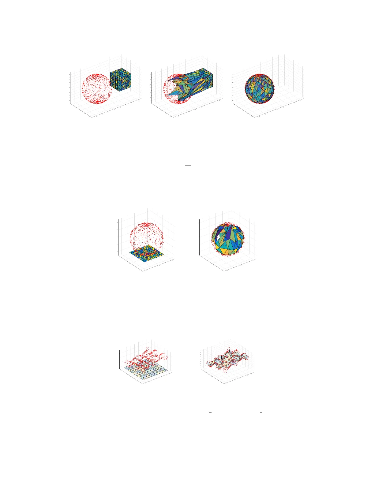
FITTING A SIMPLICIAL COMPLEX USING A V ARIA TION OF k-MEANS PIOTR BEBEN Abstract. W e give a simple and effectiv e t wo stage algorithm for appro ximating a point cloud S ⊂ R m by a simplicial complex K . The first stage is an iterative fitting procedure that general- izes k-means clustering, while the second stage in v olves deleting redundan t simplices. A form of dimension reduction of S is obtained as a consequence. 1. Introduction The use of simplicial complexes as a means for estimating top ology has found man y applications to data analysis in recen t times. F or example, unsup ervised learning tec hniques such as p ersisten t homology [4, 6] often use what are known as Cech or Vietoris-Rips filtrations to capture m ulti- scale topological features of a p oin t cloud S ⊂ R m . The simplicial complexes in these filtrations individually are not alw ays a goo d representation of the actual ph ysical shap e of S since, for example, they often ha v e a higher dimension than R m . Our aim is to giv e an algorithm that can appro ximate S to the greatest extent p ossible when fed an y simplicial complex K mapp ed linearly in to R m . This algorithm has several nice prop erties, including a tendency tow ards preserving embeddings, as w ell as reducing to k-means clustering when K is 0-dimensional. The resulting fitting is further refined b y deleting simplices that ha v e been po orly matched with S ; the end result b eing a lo cally linear appro ximation of S . A low er dimensional representation of S in terms of barycentric co ordinates follo ws by pro jecting on to this approximation. 2. Algorithm Description Fix K b e a (geometric) simplicial complex, and let { v 1 , . . . , v n } ∈ K b e the set of vertices of K . The fac ets of K are the simplices of K that hav e the highest dimension in the sense that they are not contained in the b oundary of any other simplex. K may then b e represented as a collection of facets, eac h of which is represented by the set of vertices that it contains. The dimension of a facet is equal to the n um ber of v ertices it contains min us 1. When we refer to the b oundary ∂ σ of a simplex σ , w e mean the union of its smaller dimensional b oundary simplices, even when the simplex is em b edded as a subset of R m . Its interior int ( σ ) is σ minus this boundary . An y p oin t x ∈ K is con tained in a unique smallest dimensional simplex σ x ⊆ K . W e may represen t x uniquely as a conv ex com bination x =  v j ∈ σ x λ j x v j o ver the vertices v j that are contained in σ x , where  v j ∈ σ x λ j x = 1 for some b aryc entric c o or dinates λ j x ≥ 0. A map g ∶ K Ð → R is said to b e line ar if it is linear on each simplex of K . Namely , g ( x ) =  v j ∈ σ x λ j x g ( v j ) . So g restricts to a linear em bedding on each simplex of K , and is uniquely determined by the v alues g ( v j ) that it tak es on its v ertices v j . Thus, w e ha ve a con v enient representation of g in terms of the g ( v j ) ’s. Key words and phr ases. dimensionality reduction, k-means, clustering, unsup ervised learning. 1 2 PIOTR BEBEN 2.1. Fitting. Fix S ⊂ R m our finite set of data p oin ts. Supp ose f ∶ K Ð → R m is any choice of linear map, meant to represent our initial fitting of K to S . Starting with f , our aim is to obtain successiv ely b etter fittings f ` ∶ K Ð → R m of K to S , at eac h iteration giving a b etter reflection of the shap e and structure of S . W e do this as follows. Algorithm 1 (Simplicial Means) First stage: fitting K to S 1: set f 0 ← f and ` ← − 1; 2: rep eat 3: incremen t ` ← ` + 1; 4: for each y ∈ S do 5: find a c hoice of y ′ ∈ K such that f ` ( y ′ ) is nearest to y , and σ y ⊆ K the smallest dimensional simplex that con tains y ′ ; 6: compute λ j y ≥ 0 such that  v j ∈ σ y λ j y = 1 and y ′ is the con vex com bination y ′ =  v j ∈ σ y λ j y v j . 7: end for 8: using f ` , construct a new linear map f ` + 1 ∶ K Ð → R m , defined on each vertex v j b y setting f ` + 1 ( v j ) ← 1  N ` j   y ∈ N ` j  ( 1 − λ j y ) f ` ( v j ) + λ j y y  when  N ` j  > 0, and f ` + 1 ( v j ) ← f ` ( v j ) otherwise, where N ` j ∶ = { y ∈ S  v j ∈ σ y } . 9: un til a given stop condition has not b een reac hed (e.g. max j  f ` + 1 ( v j ) − f ` ( v j ) is small) 10: set g ← f ` ; 11: return g , each σ y , y ′ , and the barycentric co ordinates λ j y . The  N ` j  > 0 assignment for f ` + 1 ( v j ) in Step 8 can b e generalized to f ` + 1 ( v j ) ← 1  N ` j   y ∈ N ` j   1 − λ j y 1 + s  f ` ( v j ) +  λ j y + s 1 + s  y  where s ≥ 0 is the le arning r ate . Larger v alues for s lead to faster conv ergence, but p oorer fittings and reduced stabilit y . T aking s to b e small ( ≤ 0 . 1) but nonzero has ev ery adv an tage in addition to prev enting the c hange in the mapping of a vertex v j b ecoming sluggish betw een iterations when the barycen tric co ordinates λ j y are all near zero. On the other hand, this do es not preven t mapping of v j from b ecoming stuck in its current p osition when each λ j y is zero (regardless of the v alue s ) since N ` j consists only of those y ∈ S for whic h y ′ is on the in terior of some simplex σ that con tains v j (meaning those on the b oundary faces of σ opp osite to v j are ignored). There are adv an tages and disadv antages to this. On the p ositiv e side, higher dimensional simplices are often preven ted from b eing collapsed onto low er dimensional linear patches of data, but this can also b e prev ent simplices from b eing fitted in situations where it would b e desired. F or example, when fitting K homeomorphic to a sphere to data sampled from a sphere (Figure 6), cr aters can form and remain in subsequent iterations if data p oin ts surrounding the crater are in fact nearest to p oin ts lying on its rim. This issue can b e circumv ented (but our adv antages reversed!) by taking the sligh tly larger set N ` j = { y ∈ S  y ′ ∈ σ for some simplex σ such that v j ∈ σ } in place of N ` j , together with s > 0. FITTING A SIMPLICIAL COMPLEX USING A V ARIA TION OF k-MEANS 3 There is a straightforw ard intuition underlying Algorithm 1. Consider the case where at the ` th iteration f ` is a linear embedding. Then v j and K can then b e thought of as f ` ( v j ) and the subspace f ` ( K ) ⊆ R m , and Algorithm 1 in essence has S attract K to wards it b y ha ving eac h point y ∈ S exert a pull on a nearest p oin t y ′ ∈ K . The ca v eat here is that in doing so the em b edding f ` m ust be k ept linear, so the net effect of this pull m ust come down to its influence on the individual v ertices v j of the simplex containing y ′ . The influence on each of these vertices v j should in turn decrease with some measure of distance of y ′ to v j . This is analogous to pulling on a string attac hed at some p oin t along a p erp endicular uniform ro d floating in space, in whic h case the acceleration of an endp oin t of the ro d in the direction of the pull decreases with increasing distance from the string. Since the size or shape of the simplex in our context is irrelev an t, the distance from y ′ to v j is measured in terms of its barycentric co ordinates λ j y . In particular, if y ′ lies near a b oundary simplex opp osite to v j , then λ j y is near 0 and y has little influence on v j , while y has full influence on v j when λ j y = 1, or equiv alently , when y ′ = v j . The accum ulation of these pulling forces on a v ertex v j leads us to take the centroid of the ( 1 − λ j y ) v j + λ j y y ov er all y ∈ N ` j ; equiv alently , ov er all y ∈ S that are closest to a p oin t y ′ lying on the interior of a simplex that has v j as a v ertex. When K is 0-dimensional – namely a collection of n disjoint vertices v j – there is only a single barycen tric co ordinate λ j y = 1 for each y ′ and N ` j =  y ∈ S  y nearest to f ` ( v j )  , so Algorithm 1 reduces to the classical k-means algorithm with initial clusters f 0 ( v j ) . Algorithm 1 is thereby a high dimensional non-discrete generalization of k-means clustering. This is perhaps in the same spirit as p ersisten t homology is a higher dimensional generalization of hierarchical clustering (also b y w ay of simplicial complexes). 2.2. Preserving embeddings. T o obtain a our fitting g , why not simply apply the k-means al- gorithm to the vertices f ( v j ) ? This would lik ely b e a p oor fitting of K since the arrangement of simplices comprising K is ignored completely . Moreo ver, g would probably not b e an embedding irresp ectiv e of f . T ake for example the case where K is the following four-vertex graph em b edded in R m = R 2 ● a GFED @ABC v 1 GFED @ABC v 2 q q q q q q q q q q q q q q M M M M M M M M M M M M M M ● b GFED @ABC v 3 GFED @ABC v 4 ● c ● y and S = { a, b, c, y } ⊂ R 2 . The nearest vertex to a , b , c , and y is v 1 , v 3 , v 4 , and v 2 resp ectiv ely , so one iteration of k-means on this data results in the edge { v 1 , v 2 } intersecting the edge { v 3 , v 4 } . On the other hand, the nearest p oin t to y in K lies on the edge { v 3 , v 4 } , so a single iteration of Algorithm 1 res ults in K b eing stretched out tow ards S without violating its em b edding. In fact, for non-pathological K , Algorithm 1 has a strong tendency to retain g ∶ K Ð → R m (and eac h f ` ) as em b eddings, giv en that the initial fitting f ∶ K Ð → R m is an em b edding. 2.3. Refinemen t. Once we ha v e obtained a sufficiently go od fitting g ∶ K Ð → R m from Algorithm 1, the next step is to refine it by getting rid of redundant simplices. These are the simplices σ ⊆ K 4 PIOTR BEBEN whose linearly embedded image g ( σ ) has no p oin ts g ( y ′ ) ∈ g ( σ ) positioned near its interior, but instead, near its b oundary ∂ g ( σ ) = g ( ∂ σ ) . W e then pro ject those g ( y ′ ) near the b oundary in to one of the simplices on the b oundary in order to obtain a lo w er dimensional approximate representation of y . This pro cess is rep eated for the pro jections. Algorithm 2 Second stage: deleting redundant simplices, reducing dimension 1: input: a threshold v alue α ≥ 0, and each y ′ , σ y , and g ∶ K Ð → R m from Algorithm 1; 2: for each y ∈ S do 3: set z ← y ′ and σ ← σ y ; 4: while σ is not a vertex do 5: find a c hoice of ˜ z in ∂ σ such that g ( z ) is nearest to g ( ˜ z ) , and ˜ σ ⊆ ∂ σ the smallest dimensional b oundary simplex that con tains ˜ z ; 6: if  g ( ˜ z ) − g ( z ) ≤ α then 7: set z ← ˜ z and σ ← ˜ σ ; 8: else 9: exit the while lo op; 10: end if 11: end while 12: set ˜ y ← z and ˜ σ y ← σ , and ˜ λ j y (for eac h v j ∈ ˜ σ y ) the barycen tric co ordinates of ˜ y in ˜ σ y ; 13: end for 14: set ˜ K ←  y ∈ S ˜ σ y ; 15: return ˜ K , and eac h ˜ y , ˜ σ y , and ˜ λ j y . The output ˜ K is a sub complex of K with g ∶ K Ð → R m restricting to a linear map g ∶ ˜ K Ð → R m , and if g is a go od fitting, g ( ˜ K ) is a locally linear approximation of S , and each g ( ˜ y ) will be a close appro ximation of the corresponding y ∈ S . The distance threshold α is fixed for simplicit y . A better c hoice would b e to hav e it monotonically decrease in eac h iteration to counteract the effect of the distance betw een y ′ and g ( z ) increasing in each iteration. Alternativ ely , a scale indep enden t measure that is more toleran t of noise in larger scale structures might b e desirable. This can b e obtained for example b y taking the minimum of the barycen tric co ordinates of y ′ in σ as a measure of nearness t o the b oundary . Algorithm 2 also alw a ys keeps those simplices that ha ve at least one point y ′ near its in terior with resp ect to α , though we could opt for something less sensitive to compromise accuracy for simplicit y . Dep ending on how many simplices are deleted from K to get to ˜ K , and ho w far do wn w e go in pro jecting each g ( y ′ ) into b oundary simplices, ˜ K will typically hav e low er dimensional facets than K . At the same time, its facets and simplices t ypically ha ve lo wer dimension than R m , so each y will ha ve a low er dimensional approximate represen tation in terms of the barycen tric coordinates ˜ λ j y of ˜ y in ˜ σ y . F or example, if ˜ σ y happ ens to be a 1-dimensional simplex (edge) with v ertices v j 1 and v j 2 , then y ≈ g ( ˜ y ) = tg ( v j 1 ) + ( 1 − t ) g ( v j 2 ) where ( t, 1 − t ) ∈ R 2 are the barycentric co ordinates of ˜ y in ˜ σ y . y can then b e appro ximately represen ted b y the barycen tric coordinates ( t, 1 − t ) together with an assignmen t of simplex y ↦ ˜ σ y (i.e. an assignmen t of those v ertices in ˜ σ y ). In summary , p oin ts y ∈ S are assigned to linear combinations  v j ∈ σ y ˜ λ j y g ( v j ) where ˜ λ j y are the barycentric co ordinates of of ˜ y in ˜ σ y . This often gives a muc h more compact represen tation of S , especially when m is large and large patches of p oints in S lie on appro ximately linear subspaces of considerably low er dimension than m . FITTING A SIMPLICIAL COMPLEX USING A V ARIA TION OF k-MEANS 5 2.4. Some comparisons. This approac h to dimension reduction is similar to that taken by k- means and self-organizing maps (SOM) [10, 9]. The assignmen t of v ertices ( no des , neur ons , classes , or clusters , in different language) how ev er do es not ha ve to b e discrete, so the reduction is not necessarily one to dimension 0 for every y ∈ S . Instead, it can b e seen as a form of F uzzy k- means [2, 20] – in this case, m ultiple vertices in g ( ˜ K ) are assigned to y to v arying degrees, this dep ending on which simplex is nearest to y and where (in terms of barycentric co ordinates) the nearest p oin t y ′ lies inside this simplex. Like SOM, the mapping g is top ology preserving, with adjacen t vertices of K and ˜ K tending to hav e nearby p oin ts in S assigned to them. SOM ho w ever acts directly on individual vertices b y matching data points with nearest vertices instead simplices, and uses an explicit neighbourho od function on nearb y v ertices to effect this prop ert y . Since simplicial complexes are able to more efficiently reflect the shape of an ob ject such as our p oint cloud S , one w ould exp ect that Algorithms 1 and 2 giv e a b etter appro ximation of S than classical SOM, at the same time using fewer v ertices. This is all at the exp ense of our dimension reduction generally being ab o ve dimension 0 dep ending on ˜ K . The end result of Algorithms 1 and 2 is that lo cal patc hes in S are approximated by the affine subspaces of R m determined by the simplices of g ( ˜ K ) . This is similar to Cluster-PCA [7], as well as the first stage of Lo cally Linear Embedding (LLE) [13]. In Cluster-PCA a collection of affine d -dimensional subspaces of R m are iteratively fitted to their nearest p oin ts in S via PCA, while LLE uses conv ex combinations of k nearest neighbours to eac h point in S (sampled from a smoothly em b edded d -manifold) in order to obtain an approximation of a lo cal co ordinate patch. In our case S need not b e a manifold, nor do es the dimension d of the affine subspaces ha ve to b e known b eforehand. Instead, K has to b e selected to hav e a high enough dimension and enough redundant facets and vertices (but not so man y so as to ov er-fit) in order to guaran tee a goo d approximation of S . None-the-less, w e are left with a conv enien t approximation of the shap e of S in terms of ˜ K and g . These dimension reduction techniques aside, there are v arious shap e approximation techniques kno wn to the computer graphics com m unity , where, for example, a mesh is iterativ ely fitted to data b y solving certain least-squares optimization problems [8]. 2.5. F urther dimension reduction. If g ∶ ˜ K Ð → R m happ ens to b e an embedding and ˜ K has dimension d with d muc h smaller than m , then one w ould lik e to go a step further and obtain a lo w er dimensional em b edding h ∶ ˜ K Ð → R k for some d ≤ k < m that preserv es as m uc h of the prop erties of g as p ossible (preserving geo desic distance for instance when ˜ K is a manifold). Assuming our fitting g is go od, a dimension reduction of S into R k follo ws since each ˜ y ≈ y ∈ S and ˜ y is in g ( ˜ K ) . There is a history of theoretical work dealing with the question whether any embedding into R k of a d -dimensional simplicial complex ˜ K can exist in the first place (ignoring g for the time-b eing). One of the most w ell-known results is V an Kamp en’s generalization of Kurato wski’s graph planarit y condition [11, 18, 14, 19], which giv es an obstruction to embedding ˜ K into R 2 d lying in the degree 2 d cohomology of a certain delete d pr o duct sub complex of ˜ K × ˜ K . In fact, this is the largest dimension of interest since any simplicial complex of dimension d can b e em b edded linearly into R 2 d + 1 (for instance, by mapping each vertex to a unique p oin t on the parametric curve ( t, t 2 , . . . , t 2 d + 1 ) ). Some more recen t w ork has focused on PL-em bedding into R d + 1 [3], or the tractability of em b edding as a decision problem [12]. A direct computational approac h is p ossible when g ( ˜ K ) is a triangulation of an em b edded mani- fold; for example, b y applying Isomap [17] to its v ertices g ( v j ) and some c hoice of samples in g ( ˜ K ) . Since the en tire manifold g ( ˜ K ) is already giv en, the geo desic distances betw een the samples can be giv en exactly , and what remains is the MDS stage of Isomap. In any case, g ( ˜ K ) is not a sampled space, and moreov er, it is often a muc h simpler ob ject than S consisting of a m uch smaller collec- tion of v ertices and facets. Any dimension reduction of S by first reducing the dimension of the em b edding of ˜ K should b e easier compared to a more head-on approach. 6 PIOTR BEBEN 2.6. Complexit y. The computationally in tensive step that dominates Algorithm 1 inv olves finding the p oin ts y ′ ∈ K for which f ` ( y ′ ) is nearest to y ∈ S . These p oin ts can b e found as follows. Algorithm 3 Find nearest p oin ts on a simplex along with their barycentric coordinates 1: input: S ⊂ R m , a simplex σ ⊆ K , and linear map f ` ∶ K Ð → R m ; 2: if σ is a vertex v j then 3: set λ σ 1 y ← 1 and y σ ← f ` ( v j ) for eac h y ∈ S ; 4: else 5: let r ∶ =  S  and pick some ordering of S = { y 1 , . . . , y r } ; 6: Let M b e the m × d matrix whose i th column is the vector w i + 1 − w 1 , where { w 1 , . . . , w d + 1 } ⊆ { f ` ( v 1 ) , . . . , f ` ( v n )} are the vertices of f ` ( σ ) ; 7: Let S b e the m × r matrix whose j th column is the vector y j − w 1 ; 8: compute the Moore-Penrose pseudoin v erse ¯ M of M , the d × r matrix B ∶ = ¯ M S , the 1 × r matrix B ′ whose j th en try is 1 − ∑ i B ij , and tak e the ( d + 1 ) × r matrix B ∶ =  B ′ B  ; 9: partition S into disjoin t subsets ¯ S and S 1 , . . . , S d + 1 where S k ∶ = { y j ∈ S  ( B ) kj < 0 } −  i < k S i and ¯ S ∶ = S −  i S i ; 10: for eac h y j ∈ ¯ S , set λ σ iy j ← ( B ) ij for 1 ≤ i ≤ d + 1, and y σ j ← ∑ i λ σ iy j ω i ; 11: for each S k that is non-empt y do 12: let σ k b e the boundary simplex of σ containing ev ery vertex w i except w k , and set λ σ ky j ← 0; 13: rep eat this algorithm for σ k in place of σ and S k in place of S , letting y σ ∶ = y σ k and λ σ iy ∶ = λ σ k iy (for i ≠ k ) denote its output for each y ∈ S k ; 14: end for 15: end if 16: output: y σ and λ σ iy for eac h y ∈ S . The output y σ is the nearest p oint to y lying on f ` ( σ ) , and the λ σ iy ’s are its barycentric co ordinates in f ` ( σ ) . The smallest dimensional simplex σ y ⊆ σ for which y σ is in f ` ( σ y ) can quic kly b e found b y lo oking at whic h of the λ σ iy ’s are zero. The pro duct ¯ M S and pseudoinv erse ¯ M can b e determined using singular v alue decomp osition of M in O ( dmr ) time and O ( min { m 2 d, md 2 }) time resp ectiv ely , so all steps b efore the final for- lo op can b e executed in O ( dmr + min { m 2 d, md 2 }) . T ypically r ≥ max { m, d } , in which case this simplifies to O ( dmr ) . Since the recursive call in each iteration of the for-lo op is executed only for those dimension d − 1 boundary simplices σ i ⊆ σ for which S i is non-empty , and since the S i ’s are all disjoin t subsets of the current input S , then at most r d = min { r, ( d + 1 ) ! } recursive calls are made. So the total execution time of the ab o v e algorithm is O ( dmrr d ) . The nearest p oint f ` ( y ′ ) to y is given as a choice of y σ o ver all facets (not simplices) of σ ⊆ K that minimizes  y σ − y  ( y ′ itself is determined b y the λ σ iy ’s). As a result, the time complexit y of eac h iteration of Algorithm 1 is at worst O ( N dmrr d ) when r ≥ max { m, d } , where N is the num b er of facets of K and d is the dimension of the highest dimensional facet in K . This is largely due to the cost of finding eac h y ′ and y σ precisely . Significant impro vemen ts can be made if an appro ximation sc heme is used. F or example, since f ` do es not c hange muc h in consecutiv e iterations in Algorithm 1 for large enough ` , y ′ can b e approximated in the ( ` + 1 ) th iteration by searching only those facets FITTING A SIMPLICIAL COMPLEX USING A V ARIA TION OF k-MEANS 7 adjacen t to the simplex that contains y ′ in the previous iteration. In effect, this means sending an appropriate subset S σ ⊆ S in place of S as input for Algorithm 3. At the same time, Algorithm 1 is easy to parallelize, since Algorithm 3 can b e applied sim ultaneously to eac h facet σ of K . 3. Some Examples on Synthetic Da t a Algorithm 1 was tested without the pruning stage (Algorithm 2). This was done on data S sampled from 1, 2, and 3 dimensional spaces using grids, triangulated meshes, or their b oundaries K embedded into R 2 , R 3 , and R 4 . Precise v alues for nearest p oin ts were found using Algorithm 3, without an y form of appro ximation, while the learning rate s w as set at 0 . 1. Implemen tation is in MA TLAB R2015b. Source co de can b e found at https://github.com/pbebenSoton/smeans . 0 0.5 1 1.5 2 0 0.5 1 1.5 (a) 0 iterations 0 0.5 1 1.5 2 0 0.5 1 1.5 (b) 20 iterations 0 0.5 1 1.5 2 0 0.5 1 1.5 (c) 150 iterations Figure 1. 200 p oints sampled from a Swiss r ol l , K a 1-dimensional 5 × 5 grid. The edges con taining no p oints near their in terior are deleted during the pruning stage. -0.6 -0.4 -0.2 0 0.2 0.4 0.6 0.8 1 0 0.2 0.4 0.6 0.8 1 1.2 1.4 1.6 1.8 (a) 0 iterations -0.6 -0.4 -0.2 0 0.2 0.4 0.6 0.8 1 0 0.2 0.4 0.6 0.8 1 1.2 1.4 1.6 1.8 (b) 200 iterations Figure 2. 200 p oin ts sampled from a Swiss roll, K a line sub divided into 60 segmen ts. The quality of this fitting is similar to classical SOM. T aking a grid of ambien t dimension as in Figure 1 gives b etter results with fewer vertices and a similar n umber of facets. 8 PIOTR BEBEN -1 -0.5 0 0.5 1 1.5 2 2.5 -1 -0.8 -0.6 -0.4 -0.2 0 0.2 0.4 0.6 0.8 1 (a) 0 iterations -1 -0.5 0 0.5 1 1.5 2 2.5 -1 -0.8 -0.6 -0.4 -0.2 0 0.2 0.4 0.6 0.8 1 (b) 150 iterations Figure 3. 200 points sampled from a unit circle, K a square with eac h side divided in to 4 segments. Fitted using the sets N ` j in place of N ` j . -3 -2 -1 0 1 2 3 -3 -2 -1 0 1 2 3 (a) 0 iterations -3 -2 -1 0 1 2 3 -3 -2 -1 0 1 2 3 (b) 100 iterations Figure 4. 300 p oin ts sampled noisily from a circle and a line, K a triangulated 6 × 6 mesh. -0.5 0 0.5 1 1.5 2 2.5 -0.5 0 0.5 1 1.5 2 2.5 (a) 0 iterations -0.5 0 0.5 1 1.5 2 2.5 -0.5 0 0.5 1 1.5 2 2.5 (b) 150 iterations Figure 5. A noisy sampling of 350 p oin ts containing a circle, and K a disjoint union of tw o 3 × 3 mesh clusters . Suc h clusters result in b etter fittings for highly disjoin t data (compared to a single large mesh). FITTING A SIMPLICIAL COMPLEX USING A V ARIA TION OF k-MEANS 9 2.5 -1 2 -0.8 -0.6 1 1.5 -0.4 -0.2 0 1 0.5 0.2 0.4 0.6 0.5 0.8 0 1 0 -0.5 -0.5 -1 -1 (a) 0 iterations 2.5 -1 2 -0.8 -0.6 1 1.5 -0.4 -0.2 0 1 0.5 0.2 0.4 0.6 0.5 0.8 0 1 0 -0.5 -0.5 -1 -1 (b) 10 iterations 2.5 -1 2 -0.8 -0.6 1 1.5 -0.4 -0.2 0 1 0.5 0.2 0.4 0.6 0.5 0.8 0 1 0 -0.5 -0.5 -1 -1 (c) 150 iterations Figure 6. 1000 points sampled from a unit 2-sphere, K the triangulated boundary of a 5 × 5 × 5 mesh. Fitted using the sets N ` j in place of N ` j . -1 1 -0.5 0 0.5 1 0.5 0.5 0 1 0 -0.5 -0.5 -1 -1 (a) 0 iterations -1 1 -0.5 0 0.5 1 0.5 0.5 0 1 0 -0.5 -0.5 -1 -1 (b) 150 iterations Figure 7. 800 p oin ts noisily sampled from a unit 2-sphere, K a triangulated 8 × 8 mesh. -1 -0.5 1.5 0 1 0.5 1.5 0.5 1 0 0.5 0 -0.5 -0.5 -1 -1 -1.5 -1.5 (a) 0 iterations -1 -0.8 -0.6 1.5 -0.4 -0.2 0 0.2 1 0.4 0.6 1.5 0.8 0.5 1 0 0.5 0 -0.5 -0.5 -1 -1 -1.5 -1.5 (b) 40 iterations Figure 8. 1000 points sampled from the surface 1 3 cos ( 5 x ) sin ( 5 y ) + 1 5 ( x − y ) , K a triangulated 9 × 9 mesh. 10 PIOTR BEBEN -2 2 -1.5 -1 1.5 -0.5 2 1 0 1.5 0.5 0.5 1 1 0 0.5 1.5 0 -0.5 2 -0.5 -1 -1 -1.5 -1.5 -2 -2 (a) 0 iterations -2 2 -1.5 -1 1.5 -0.5 2 1 0 1.5 0.5 0.5 1 1 0 0.5 1.5 0 -0.5 2 -0.5 -1 -1 -1.5 -1.5 -2 -2 (b) 40 iterations Figure 9. 300 points noisily sampled from a 2-sphere and a line, K a triangulated 3 × 3 × 3 mesh (solid cub e). 0 5 10 15 20 25 30 iterations 0 0.5 1 1.5 2 2.5 3 mean sum squared distances 3D mesh 4D mesh boundary Figure 10. S tak en as 2000 p oints noisily sampled from a unit 3-sphere embedded in 4-dimensional euclidean space R 4 , and K resp ectiv ely a triangulation of a 4 × 4 × 4 mesh, and the b oundary of a 3 × 3 × 3 × 3 mesh. The mean sum of squared distances in eac h iteration is taken betw een points in S and their corresp onding nearest p oin ts in the curren t fitting of K . 4. Discussion F or non-pathological complexes K (suc h as ab ov e) Algorithm 1 quickly con verges to a stable fitting. In most cases it also preserves the embedding of K , and where it do es not, then it is usually very close to an embedding, with only a few simplices in tersecting ov er a relatively small area (in tersections are more common for less noisy data). All of these properties are less likely hold for irregularly triangulated K ; for example, when the degree of some vertices is muc h higher than others. If there is conv ergence, what is the ob jective function that is b eing minimized? Since Algo- rithm 1 generalizes k-means clustering, an obvious first choice is the sum of squared distances d ` = ∑ y ∈ S  y − f ` ( y ′ ) 2 . Indeed, there are cases where this function happ ens to b e minimized b et ween every successive iteration; for instance, in the example in Figures 8 and 10. On the FITTING A SIMPLICIAL COMPLEX USING A V ARIA TION OF k-MEANS 11 other hand, if w e start off as in Figure 4, with ` = 0 and f 0 ( K ) containing every p oin t in S , then f ` ( K ) is unlik ely to con tain S for large enough ` , so d ` will not alw ays minimized. In this situation it app ears more appropriate to consider the Hausdorff distance d H ( S , f ` ( K )) = inf   ≥ 0  f ` ( K ) ⊆ ( S )  and S ⊆ ( f ` ( K ))   where A  is the  -neighbourho o d of a subset A ⊆ R m . In an y case, it is not immediately clear what the ob jectiv e function might b e, or if there even is a single one. Another question is: under what mo difications to Algorithm 1 is preserv ation of embedding guaran teed for some given (or all) K ? One p ossibilit y is to assume all facets of K ha ve the same am bient dimension m as R m , then to update the v ertices f ` ( v j ) in each iteration one at a time – at eac h up date step considering only those y ∈ N ` j that are inside a con vex neighbourho o d B of f ` ( v j ) , where B is con tained in the union of the (currently updated) facets which ha v e f ` ( v j ) as a v ertex. This can b e shown to preserve embedding, it keeps vertices on the b oundary fixed, and therefore p oin ts y that are inside f ` ( K ) remain as such in subsequen t iterations. Then in order to get a go o d fitting, a large enough triangulation of (say) an m -ball K is selected, together with a sufficien tly expansiv e initial embedding f such that: there are enough interior facets in K to approximate S . The main do wnside to this approach is that K would ha ve to be infeasibly large when m is large. As with k-means clustering, there is the issue of selecting the appropriate n umber of clusters (v ertices) to start with. On top of this there are many other factors, such as the num b er, dimension, and the arrangement of facets that go into describing our simplicial complex K . Ideally , K w ould b e taken to b e a mesh of dimension d with a fine enough sub division, embedded into R d so as to con tain S . Such choice K represen ts a brute force approach, where the guarantee of a go od fitting is the result of a high density of redundant simplices spread out uniformly in R d . F or large d this is of course impractical – even the smallest triangulation of the 15-cub e has 2 15 v ertices and o ver ten million facets of dimension 15, increasing exp onentially with d [15]. On the other hand, a simplex of an y dimension d has only one facet and d + 1 v ertices, so there is plent y of room for compromise. Skirting this issue by selecting the mesh K to ha ve few er sub divisions or a low er dimension can leav e a large subset S ′ of points in S p oorly appro ximated b y the final fitting g of K (see Figures 7 and 9 for example). One wa y around this is to fit a new complex K ′ to the subset S ′ , but this runs the risk of S ′ b eing a po or sampling of the underlying space. So there migh t be nothing meaningful left to fit. Instead, we can consider a gr owing pro cedure akin to growing SOM (GSOM) [1]: (1) first b y considering the set C of those simplices σ ⊆ K for which g ( σ ) is a po or appro ximation of the p oin ts y ∈ S nearest to its interior (i.e.  y ′ ∈ int ( σ )  y − g ( y ′ ) is large); (2) forming a new complex K ′ from K b y attac hing a ( k + 1 ) -dimensional simplex to each k dimensional simplex in C ; (3) extending g to a linear map g ′ ∶ K ′ Ð → R d ; (4) then refitting K ′ to S starting with g ′ as our initial fitting. Simplices are the smallest ob jects that can b e attached; a more robust alternative w ould b e to form K ′ from K by attac hing a triangulation of the pro duct L × ∆ 1 =  ( x, y )  x ∈ L, y ∈ ∆ 1  to the sub complex L =  σ ∈ C σ , where ∆ 1 is the 1-simplex (an edge). In either approach we increase the dimension of K lo cally in order to capture the spread of local patc hes of data in S . Then reapplying the pruning stage (Algorithm 2) just as we did before captures the underlying structure. References 1. D. Alahakoon, S. K. Halgamuge, and B. Siriniv asan, A self gr owing cluster development appr o ach to data mining , Proceedings of IEEE International Conference on Systems, Man and Cybernetics 3 (1998), 2901–2906. 2. James C. Bezdek, Pattern r e c ognition with fuzzy obje ctive function algorithms , Kluw er Academic Publishers, Norwell, MA, USA, 1981. 3. A. Bj¨ orner and A. Goo darzi, On Co dimension one Emb e dding of Simplicial Complexes , ArXiv e-prints (2016). 4. Gunnar Carlsson, T op olo gy and data , Bull. Amer. Math. So c. (N.S.) 46 (2009), no. 2, 255–308. MR 2476414 5. L. Cayton, Algorithms for manifold le arning , Univ. of California at San Diego T ech. Rep (2005). 6. Herb ert Edelsbrunner and John Harer, Persistent homolo gy—a survey , Surveys on discrete and computational geometry , Con temp. Math., vol. 453, Amer. Math. So c., Providence, RI, 2008, pp. 257–282. MR 2405684 12 PIOTR BEBEN 7. K. F ukunaga and D. R. Olsen, A n algorithm for finding intrinsic dimensionality of data , IEEE T rans. Comput. 20 (1971), no. 2, 176–183. 8. Hugues Hopp e, T ony DeRose, T om Duc hamp, John McDonald, and W erner Stuetzle, Mesh optimization , Pro- ceedings of the 20th Ann ual Conference on Computer Graphics and In teractiv e T echniques (New Y ork, NY, USA), SIGGRAPH ’93, ACM, 1993, pp. 19–26. 9. T. Kohonen, M. R. Schroeder, and T. S. Huang (eds.), Self-or ganizing maps , 3rd ed., Springer-V erlag New Y ork, Inc., Secaucus, NJ, USA, 2001. 10. T euvo Kohonen, Self-or ganize d formation of top olo gic al ly c orr e ct featur e maps , Biological Cyb ernetics 43 (1982), no. 1, 59–69. 11. Casimir Kuratowski, Sur le pr oblme des c ourb es gauches en top olo gie , F undamenta Mathematicae 15 (1930), no. 1, 271–283 (fre). 12. Jir ´ ı Matousek, Martin T ancer, and Uli W agner, Har dness of emb edding simplicial c omplexes in r d , CoRR abs/0807.0336 (2008). 13. Lawrence K. Saul and Sam T. Row eis, Think glob al ly, fit lo c al ly: Unsup ervise d learning of low dimensional manifolds , J. Mach. Learn. Res. 4 (2003), 119–155. 14. Arnold Shapiro, Obstructions to the imb e dding of a c omplex in a euclide an sp ac e. I. The first obstruction , Ann. of Math. (2) 66 (1957), 256–269. MR 0089410 15. W arren D. Smith, A lower b ound for the simplexity of then-cube via hyperb olic volumes , Europ ean Journal of Combinatorics 21 (2000), no. 1, 131 – 137. 16. C. O. S. Sorzano, J. V argas, and A. P . Montano, A survey of dimensionality r e duction techniques , ArXiv e-prints (2014). 17. J. B. T enenbaum, V. de Silv a, and J. C. Langford, A glob al geometric fr amework for nonlinear dimensionality r e duction , Science 290 (2000), 2319–2323. 18. E. R. v an Kamp en, Komplexe in euklidischen R¨ aumen , Abh. Math. Sem. Univ. Hamburg 9 (1933), no. 1, 72–78. MR 3069580 19. W u W en-ts ¨ un, A the ory of imb e dding, immersion, and isotopy of p olytop es in a euclide an sp ace , Science Press, Peking, 1965. MR 0215305 20. M.-S. Y ang, A survey of fuzzy clustering , Mathematical and Computer Mo delling 18 (1993), no. 11, 1 – 16. School of Ma thema tics, University of Southampton, Southampton SO17 1BJ, United Kingdom E-mail address : P.D.Beben@soton.ac.uk; pdbcas@gmail.com