Identifiability and testability in GRT with Individual Differences

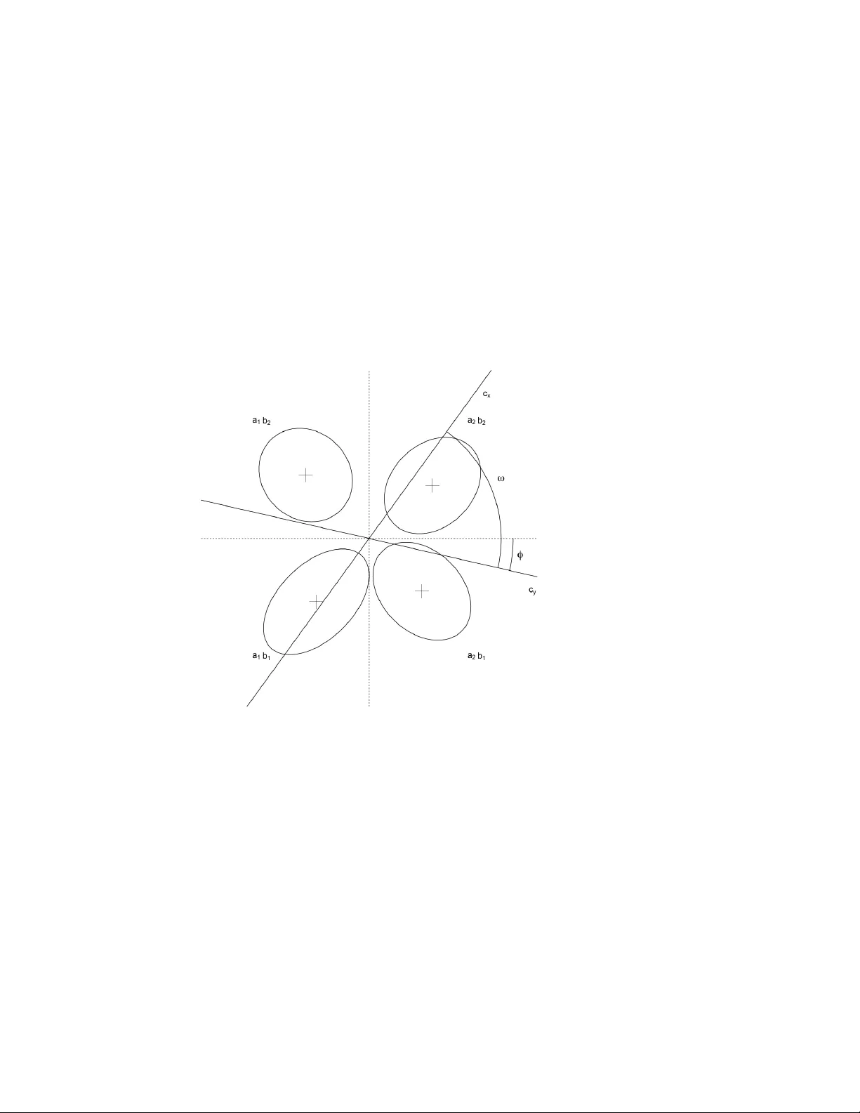
Identifiability and testability in GR T with Indi vidual Di ff erences Noah H. Silbert a , Robin D. Thomas b a Department of Communication Sciences and Disor ders, University of Cincinnati b Department of Psychology , Miami University Abstract Silbert and Thomas (2013) sho wed that failures of decisional separability are not, in general, identifiable in fully parameterized 2 × 2 Gaussian GR T models. A recent exten- sion of 2 × 2 GR T models (GR T wIND) was dev eloped to solve this problem and a con- ceptually similar problem with the simultaneous identifiability of means and marginal variances in GR T models. Central to the ability of GR T wIND to solve these problems is the assumption of universal per ception , which consists of shared perceptual distri- butions modified by attentional and global scaling parameters (Soto et al., 2015). If univ ersal perception is valid, GR T wIND solv es both issues. In this paper, we sho w that GR T wIND with uni versal perception and subject-specific f ailures of decisional separa- bility is mathematically , and thereby empirically , equiv alent to a model with decisional separability and failure of uni versal perception. W e then provide a formal proof of the fact that means and marginal variances are not, in general, simultaneously identifiable in 2 × 2 GR T models, including GR T wIND. These results can be taken to delineate precisely what the assumption of univ ersal perception must consist of. Based on these results and related recent mathematical dev elopments in the GR T framew ork, we pro- pose that, in addition to requiring a fixed subset of parameters to determine the location and scale of any giv en GR T model, some subset of parameters must be set in GR T mod- els to fix the orthogonality of the modeled perceptual dimensions, a central conceptual underpinning of the GR T frame work. W e conclude with a discussion of perceptual primacy and its relationship to uni versal perception. K e ywor ds: General Recognition Theory, identifiability, testability, GR T wIND, decisional separability 1. Introduction Recent work within the general recognition theory (GR T) indicates that failures of decisional separability are not generally identifiable under common assumptions (Silbert and Thomas, 2013; Thomas and Silbert, 2014), and it has long been known that the latent perceptual means and marginal v ariances are not, in general, simultaneously identifiable in GR T models (e.g., W ickens, 1992). A recently dev eloped multilevel extension of GR T (GR T with Individual Di ff erences, or GR T wIND) has been pro ff ered as a solution to both of these problems (Soto et al., 2015; Soto and Ashby, 2015). In this Pr eprint submitted to Journal of Mathematical Psyc hology J anuary 21, 2020 theoretical note, we show that any GR T wIND model exhibiting failures of decisional separability or non-unit marginal variances is mathematically , and thereby empirically , equiv alent to a model the exhibits neither trait. GR T wIND solves these two problems only conditionally , if the assumption of of uni versal perception is valid, but the v alidity of univ ersal perception cannot be established within GR T wIND. The purpose of this note is, in no small part, to establish precisely , and mathematically , what the assumption of univ ersal perception entails. It is important at the outset to mention a subtle distinction relating to the notion of identifiability . Specifically , in this paper we will distinguish between identifiability and testability . For the present purposes, identifiability concerns the mapping between par - ticular parameter values and observ able data gi ven a particular model. 1 A set of param- eters is identifiable if, gi ven a particular model, distinct parameter values map uniquely to corresponding data. On the other hand, testability concerns the relationship between the assumptions underlying a model and the model’ s empirical consequences. The un- derlying assumptions of a model are testable if relaxation of these assumptions leads to distinct empirical predictions. 2 Although both identifiability and testability concern the assumptions and empirical consequences of a model, the two ideas are not coexten- siv e. W e show below that there are substantial testability problems in GR T wIND, and we return to these issues periodically throughout the text as they relate to the material at hand. W e be gin, in section 2, by briefly re vie wing the structure of the 2 × 2 Gaussian GR T model and two extensions of this model (the concurrent ratings and n × m idenfication models, with n , m > 2; Ashby, 1988; W ickens and Olzak, 1989, 1992). 3 In section 3, we briefly recapitulate Silbert & Thomas’ s (2013) proposition i , which describes (a subset of) the relationships between failures of decisional separability , perceptual separability , and perceptual independence. W e also recapitulate Soto et al. ’ s (2015) generalization of this proposition as it relates to models with multiple decision bounds on each dimension. In section 4, we describe the GR T wIND model and discuss its relationship to the concurrent ratings and n × m models. In section 5, we discuss the logic of testabil- ity with respect to Silbert & Thomas’ s proposition i and the assumption of univ ersal perception in GR T wIND. W e then sho w , through a minor generalization of proposition i , that any GR T wIND model with subject-specific failures of decisional separability is mathematically and empirically equiv alent to a model in which decisional separabil- ity holds and in which the assumption of univ ersal perception does not. In section 6, we gi ve a proof of a frequently stated, but, to the best of our kno wledge, not formally prov en empirical equiv alence between mean and mar ginal v ariance parameters in 2 × 2 Gaussian GR T models. The generalization of proposition i in section 5 and the proof of mean-variance equiv alence in section 6 together help delineate precisely what the 1 That is, under the assumption that the the functional form of the model and the probabilistic assumptions of the data and model parameters are true 2 Our notion of testability is closely related to the notion of structural identifiability (e.g. Bellman and strm, 1970; Eisenfeld, 1985). 3 Henceforth, we will use n × m to refer exclusiv ely to identification models with more than 2 lev els on each dimension. 2 assumption of univ ersal perception consists of and sho w that this assumption is not testable with GR T wIND and associated identification-confusion data. Finally , we discuss more general issues about the mapping between physical di- mensions and modeled psychological dimensions in GR T . W e propose that, in addition to the necessity of fixing the location and scale of GR T models, the dimensional orthog- onality of GR T models must be fix ed, as well. W e argue, following Silbert and Thomas (2013), that this is typically best done by assuming decisional separability , though we also discuss other possible approaches, noting that the scope of this assumption in single-subject identification and concurrent ratings models is straightforward, whereas it is some what less so in multilev el models lik e GR T wIND and the models described by Silbert (2012, 2014). W e conclude with a brief discussion of the relationship between univ ersal perception and the concept of perceptual primacy . 2. General Recognition Theory 2.1. GRT fundamentals GR T is a two-stage model of perception and response selection (Ashby and T ownsend, 1986; Kadlec and T ownsend, 1992; Thomas, 2001b; Silbert, 2014; W ickens, 1992). The first stage consists of noisy perception. The second stage consists of determin- istic response selection. Noisy perception is modeled with multiv ariate probability distributions defined ov er an unobserved perceptual space. Response selection is mod- eled with decision bounds, i.e., curves that exhausti vely partition the perceptual space into response regions. Any giv en perceptual e ff ect is represented as a point in percep- tual space. The response to a perceptual e ff ect is determined by the response region in which the perceptual e ff ect occurs. The probability of a particular response to a particular stimulus is modeled as the multiple integral of the perceptual distribution corresponding to the stimulus ov er an appropriate response region. 2.2. The 2 × 2 model The most common use of GR T is to analyze identification-confusion data in a 2 × 2 factorial paradigm, wherein the stimuli consist of the f actorial combination of tw o lev- els on each of two dimensions (e.g., Ashby and T o wnsend, 1986; Silbert, 2012, 2014; Thomas, 2001b,a). For example, a factorial combination of frequency and intensity could produce a set of stimulus tones that are lo w or high frequency and lo w or high intensity . In this case the four stimuli would be A 1 B 1 = low frequency , low inten- sity; A 1 B 2 = lo w frequency , high intensity; A 2 B 1 = high frequency , low intensity; and A 2 B 2 = high frequency , high intensity . Figure 1 illustrates the equal likelihood contours and decision bounds of one possi- ble 2 × 2 Gaussian GR T model. The levels of the stimuli and corresponding response regions are indicated by a i b j , with i , j ∈ { 1 , 2 } ; 4 a i indicates the lev el on the x di- mension (e.g., low vs high frequency) and b j indicates the lev el on the y dimension 4 Uppercase A i B j indicate the le vels of the stimuli and corresponding perceptual distrib utions, while lo w- ercase a i b j indicate response lev els. 3 (e.g., low vs high intensity). The vertical decision bound, c x , partitions the x -axis, and the horizontal bound, c y , partitions the y -axis. T ogether, they specify response re gions corresponding to the same factorial structure that defines the stimuli. Figure 1: 2 × 2 Gaussian GR T example illustration. This model illustrates the three dimensional interaction concepts defined in the GR T frame work: perceptual independence (PI), perceptual separability (PS), and de- cisional separability (DS). With Gaussian perceptual distrib utions, PI is equi valent to zero correlation, and failure of PI is equi valent to non-zero correlation. The top two perceptual distributions illustrate failure of PI, while the bottom two exhibit PI. PS is illustrated with respect to the y dimension. The perceptual distrib utions are perfectly horizontally aligned at each le vel of B j ; the mar ginal distrib utions of perceptual e ff ects on the y dimension do not v ary as a function of the le vel on the x dimension. By way of contrast, PS fails with respect to the x dimension; the mar ginal perceptual distrib utions on this dimension vary across levels of the y dimension. Finally , because the decision bounds are parallel to the coordinate axes, DS holds in this model. Decision bounds that are not parallel to the coordinate axes would represent a f ailure of DS. 2.3. Multi-bound extensions of the model Although the 2 × 2 Gaussian model is the most commonly used GR T model (along with the associated factorial identification experimental paradigm), extensions of this model were developed shortly after GR T was defined as such. The concurrent ratings 4 model (Ashby, 1988; W ickens and Olzak, 1989, 1992) and the n × m model (with n , m > 2) were two of the first e xtensions of GR T , and both play an important role here. A concurrent ratings model is illustrated in Figure 2. The structure of this model is very similar to the 2 × 2 model illustrated in Figure 1, with the key di ff erence that the concurrent ratings model has two or more decision bounds on each dimension. Concurrent rating models are used to analyze judgments giv en separately to each component (dimension) of the stimulus. 5 Crucially for our purposes, the number of response lev els can be greater than those that define the stimuli. For e xample, exper - iment participants may giv e ratings on a k -point scale indicating, on each dimension, the degree to which a stimulus is judged to hav e been at a low or high value. The model illustrated in Figure 2 could be used to analyze data in which subjects could respond, e.g., ‘low’, ’uncertain’, or ’high. ’ Figure 2: A concurrent ratings model with two (parallel) decision bounds on each dimension. W e refer to a closely related extension of GR T as the n × m model. Like the 2 × 2 model discussed abov e, the n × m model is used to analyze identification data, but like the concurrent ratings model, the n × m model has multiple decision bounds on each di- mension. The k ey di ff erence between the concurrent ratings and n × m model is that the latter has perceptual distributions corresponding to each response region. For example, 5 Strictly speaking, ‘concurrent’ refers to separate responses on each dimension, while ’ratings’ refers to multiple response lev els on each dimension. 5 the n × m model has been used to model data from participants’ identification of stimuli consisting of the factorial combination of three lev els on each of tw o dimensions (e.g., Ashby and Lee, 1991; Thomas et al., 2015). The 2 × 2, n × m , and concurrent ratings models were each originally designed to analyze a single subject’ s data (Ashby and Lee, 1991; Thomas, 2001b,a; W ickens and Olzak, 1989). Although the concurrent ratings and n × m model are distinct, for the present analyses we introduce the term multi-bound model , which we will use to refer to both types of model in order to distinguish them as a class distinct from the standard 2 × 2 model. It is of central importance to the present analysis that multi- bound models predict, and the data from associated tasks may contain, responses at intermediate lev els, where in the 2 × 2 identification identification paradigm, the data and model predictions consist only of ‘low’ or ‘high’ responses. 2.4. Multilevel e xtensions of the model T wo recent e xtensions of GR T ha ve focused on the simultaneous analysis of multi- ple subjects’ data. One of these extensions is a Bayesian model in which each subject’ s data is fit to a standard 2 × 2 model, while, simultaneously , the individual subjects’ parameters are modeled as random variables gov erned by group-level parameters (Sil- bert, 2012, 2014). The other extension is GR T wIND, in which a group-lev el set of parameters are shared as well as partially modified and complemented by subject-lev el parameters (Soto et al., 2015; Soto and Ashby, 2015). W e refer to these models as mul- tilevel to distinguish them as a class distinct from models designed to analyze a single subject’ s data. It is important to note that multi-bound and multile vel models are not mutually ex- clusiv e classes. Both the Bayesian multile v el model and GR T wIND could, in principle, be implemented as concurrent ratings or n × m models. As it happens, neither hav e been so implemented thus far , so, in practice, no multi-bound GR T models are multilev el, and no multilev el GR T models are multi-bound. The distinction between multi-bound and multilevel models helps elucidate the scope of Silbert & Thomas’ s proposition i and Soto et al. ’ s generalization thereof. Specifically , Silbert and Thomas (2013) show that DS, PS, and PI are not simulta- neously testable in single-subject 2 × 2 identification-confusion models. More specifi- cally , the y show that the parameters are not identifiable in a fully general Gaussian GR T model (i.e., a model in which DS, PS, and PI may all fail). Soto et al. (2015) generalize proposition i to show that this is also true of two-dimensional Gaussian GR T models with multiple bounds on each dimension if and only if the bounds on a gi ven dimension are parallel. 6 Soto et al. infer that neither proposition i nor their generalization thereof apply to GR T wIND. W e sho w belo w that this is incorrect. In the following section, we briefly recapitulate, for conv enience, the proof of pro- postion i . 7 W e also recapitulate Soto et al. ’ s generalization of this proposition. 6 Neither Silbert and Thomas (2013) nor Soto et al. (2015) distinguish between identifiability and testa- bility as we use the terms here, in both cases discussing these issues exclusi vely in terms of identifiability . 7 W e focus here on the non-testability of DS in 2 × 2 Gaussian GR T models with linear decision bounds. Although we do not address other types of decision bounds here (e.g., piecewise linear bounds), we see no 6 3. Recapitulation of Silbert and Thomas (2013), proposition i , and Soto et al. ’ s generalization thereof Silbert and Thomas (2013) showed that single-subject 2 × 2 Gaussian GR T models with linear decision bounds that are not parallel to the coordinate axes can be linearly transformed to align the decision bounds with the coordinate axes. Hence, ev ery single- subject 2 × 2 Gaussian GR T model with linear decision bounds exhibiting failure of DS is empirically equi valent to a single-subject 2 × 2 Gaussian GR T model in which DS holds. By w ay of contrast, models exhibiting failures of perceptual separability are not, in general, empirically equiv alent to models in which perceptual separability holds. 8 Mathematically , Silbert and Thomas (2013) sho wed that a model with angle φ be- tween c y and the x -axis and angle ω between c x and c y can be rotated and sheared by applying the following tw o linear transformations 9 : R = " cos φ − sin φ sin φ cos φ # (1) S = " 1 − 1 tan ω 0 1 # (2) Figures 3, 4, and 5 illustrate ho w a model with linear failure of DS can be rotated (via R ) and sheared (via S ) to induce DS. Figure 3 illustrates a model exhibiting linear failure of DS, wherein the horizontal decision bound c y deviates from the x axis by the angle φ , and the two decision bounds are separated by the angle ω . Application of the rotation R aligns c y with the x -axis, producing the model illus- trated in Figure 4. The angle ω between c x and c y is preserved by the rotation. Appli- cation of the shear transformation S preserves the alignment of c y with the x -axis and aligns c x with the y -axis, thereby inducing DS. Because these linear transformations are in vertible, the predicted response probabilities are preserved (Billingsley, 2012, pp. 215-216). Silbert and Thomas (2013) provide a formal proof of their proposition i , which states that, with linear decision bounds and a single-subject 2 × 2 Gaussian GR T model, “any perceptually separable b ut decisionally nonseparable configuration can be trans- formed to a configuration that is perceptually nonseparable, decisionally separable, and equi valent with respect to predicted response probabilities. ” Silbert and Thomas (2013) focus on the case with PS and failure of DS in order to illustrate how closely related these two notions of dimensional interaction are. Howe ver , they also note that the proposition is readily generalized to include models that do not exhibit PS prior to rotation and / or shear transformations. reason to think that they would resolve this issue if implemented in GR T wIND. Silbert and Thomas (2013) show , via simulation, that the same basic issue exists in 2 × 2 models with piecewise linear bounds. It will be clear shortly why these results also apply to GR T wIND. 8 A special case in which PS may be induced by application of linear transformations (mean-shift inte- grality) is giv en in proposition ii of Silbert and Thomas (2013) and clarified in Thomas and Silbert (2014). 9 Note that, without loss of generality , the location of the model is fixed by putting the intersection of the two decision bounds at the origin. The same rotation and shear transformations will induce DS in a non-centered model, e.g., one in which the A 1 B 1 perceptual distribution is fix ed at the origin. 7 Figure 3: 2 × 2 Gaussian GR T model exhibiting f ailure of DS. φ indicates the angle between the ‘horizontal’ decision bound c y and the x -axis. ω indicates the angle between the two decision bounds c x and c y . 8 Figure 4: Rotated 2 × 2 Gaussian GR T model. 9 Figure 5: Sheared 2 × 2 Gaussian GR T model. 10 Soto et al. (2015) generalize proposition i from Silbert and Thomas (2013) and prov e that this result also holds for Gaussian GR T models with multiple, parallel deci- sion bounds on each dimension. More specifically , as stated abov e, Soto et al. sho w that proposition i holds in two-dimensional Gaussian GR T models with more than one bound on each dimension if and only if the bounds on a giv en dimension are parallel. 10 Based on this generalization, Soto et al. (2015) write that Silbert & Thomas’ s propo- sition i “is not generally true in GR T -wIND or any other model with more than one bound per dimension. The non-identifiability of decisional separability arises in such models only under v ery specific circumstances” (p. 108). 11 They conclude, incorrectly , that failures of DS are, in general, testable in GR T wIND. Because GR T wIND is a multilev el 2 × 2 model, the decision bounds in GR T wIND do not function as multiple bounds on the same dimension in the same way that the decision bounds in a concurrent ratings or n × m model do; using the terminology introduced above, GR T wIND is not a multi-bound model. Soto et al. are correct that the transformations at the heart of proposition i cannot induce DS simultaneously for all subjects. Howe ver , proposition i applies in a subject-specific manner, such that subject- specific failures of DS in GR T wIND map one-to-one onto subject-specific rotation and shear transformations. Any GR T wIND model with univ ersal perception and subject- specific failures of DS is mathematically and empirically equiv alent to a transformed GR T wIND model with DS for all subjects and violation of univ ersal perception. 4. The structure of GR T wIND GR T wIND is a multilev el, 2 × 2 Gaussian GR T model that relies crucially on the assumption of univ ersal perception (Soto et al., 2015; Soto and Ashby, 2015). Soto et al. write that “the model assumes that the structure of the perceptual distributions is the same for all participants; that is, some aspects of perception are uni versal, in particular the relations between dimensions within stimuli (cov ariance of each distribution) and across stimuli (the means of each distribution and the ratio of their variance along a dimension).... it is also assumed that attentional and decisional processes could v ary across individuals” (p. 91). 4.1. Gr oup- and individual-level parameters Mathematically , in GR T wIND there is a shared group-lev el set of four biv ariate Gaussian perceptual distributions. Each individual subject’ s modeled perceptual dis- tributions are modifications of the shared group-lev el distributions. In addition, each individual subject has a set of linear decision bounds, each specified by an intercept and a slope. 10 T o the best of our knowledge, it has not pre viously been noted that multi-bound models with non-parallel bounds on a gi ven dimension produces uninterpretable response re gions, making them incoherent models of perception and response selection. Consider , for example, the model illustrated in Figure 2 if c y 1 and c y 2 were not parallel. Because non-parallel lines intersect, this would produce a re gion that is simultaneously above c y 2 and below c y 1 . 11 Here ‘non-identifiability’ refers to non-testability , using the terminology established above. 11 The group-level perceptual distrib ution for stimulus A i , B j has a mean vector and cov ariance matrix: µ A i B j = " µ x , A i B j µ y , A i B j # (3) Σ A i B j = " σ x x , A i B j σ xy , A i B j σ y x , A i B j σ yy , A i B j # (4) As in the the standard 2 × 2 and multi-bound models, the mean vector for one distribution is set equal to (0 , 0) T to fix the location of the model, and, as in multi- bound models, the marginal v ariances in one distribution are set equal to one to fix the scale of the model. 12 For individual subject k , the covariance matrix corresponding to stimulus A i , B j is giv en by the following equation, with κ k > 0 and 0 < λ k < 1: Σ k , A i B j =         σ x x , A i B j κ k λ k σ xy , A i B j κ k √ λ k (1 − λ k ) σ yx , A i B j κ k √ λ k (1 − λ k ) σ yy , A i B j κ k (1 − λ k )         (5) Note that, because the (absolute and relative) scaling is applied only to marginal variances, subject k ’ s mean vector for stimulus A i B j is just the group-level mean vector: µ k , A i B j = µ A i B j (6) Note, too, that although Soto et al. (2015) state, in the quote abov e, that the co vari- ance of each distrib ution is constant, the scaling and dimension-weighting parameters κ k and λ k ensure that this is not generally true. Rather, the assumption is that the cor - r elation of each distribution is constant across subjects. More generally , it is clear that the assumption of uni versal perception allows for scaling of marginal variances, both with respect to the absolute scale of the space ( κ ) and with respect to the relati ve importance of each dimension ( λ ), b ut it does not allo w for di ff erences in failures of PS or PI. Naturally enough, gi ven that it is a constraint on perceptual representations, uni versal perception also allows for di ff erences with respect to failures of DS across subjects. 4.2. GRT wIND, n × m, and concurrent r atings models In two-dimensional, Gaussian GR T models, the predicted probability of response a i b j to stimulus A k B l is gi ven by the following equation, expressed with some abuse of notation in the interest of simplicity: Pr( a i b j | A k B l ) = ¨ R a i b j N (2)  µ A k B l , Σ A k B l  d y d x (7) 12 It is typical in the standard 2 × 2 model to set all marginal variances equal to one. W e return to this issue below . 12 Here, N (2) ( µ , Σ ) indicates a biv ariate Gaussian (normal) probability density func- tion 13 with mean vector µ and cov ariance matrix Σ , and the integration is taken ov er the response region R a i b j . As discussed abov e, in a multi-bound model for a gi ven subject’ s data, a number of the response regions are determined both by decision bounds above and below (on the y -axis) and / or to the left and right (on the x axis) of the region. See, for example, the response regions at the intermediate levels a 2 or b 2 in Figure 2 above. Corresponding to this structure in the model, the data from a concurrent ratings or n × m identification task may contain responses at intermediate lev els. By w ay of contrast, no response region in the 2 × 2 GR T wIND model is determined by more than one decision bound on a gi ven dimension, and the data from the cor- responding 2 × 2 task cannot, by definition, contain responses at intermediate lev els. From the perspectiv e of subject k , the task is identical to the standard 2 × 2 factorial identification task, whether his or her data will be analyzed by GR T wIND or not. This distinction between GR T wIND and true multi-bound models is important for understanding the scope of Silbert & Thomas’ s proposition i and Soto et al. ’ s general- ization of it. It follows directly from these results that failure of DS is not generally testable in single-subject multi-bound models with parallel bounds on a gi ven dimen- sion. The rotation and shear transformations described by Silbert and Thomas (2013) apply to the whole single-subject model. But it does not then follow from this fact that failures of DS are, in general, testable in GR T wIND. In the next section, we sho w that they are not. 5. Mathematical and empirical equivalence of GRT wIND with and without deci- sional separability 5.1. The logic of testability in GRT Before providing a formal demonstration of the fact that failures of DS are not, in general, testable in GR T wIND models, we discuss some of the philosophical issues underlying identifiability and testability . As discussed above, Silbert and Thomas (2013) showed, in proposition i , that fail- ures of DS are not testable in 2 × 2 GR T models. On the other hand, only a subset of failures of PS and PI are not testable. They conclude that application of 2 × 2 GR T models should rely on the assumption of DS. A researcher follo wing their recommen- dation would be able to test failures of PS and PI, and the parameters of a Gaussian GR T model would be identifiable, conditional on the assumption that DS holds . Now , consider the follo wing logic: Suppose we assume that DS holds, and we fit a 2 × 2 GR T model and find that PS and PI fail. Can we conclude that PS and PI have failed? It is the joint hypothesis of DS + PS + PI that has been rejected, but we do not know unconditionally which antecedents are false. If our assumption that DS holds is not v alid, then our conclusions regarding the failure of PS and PI are incorrect. The set of DS, PS, and PI together is not testable. 13 In order to maintain consistenty with Silbert and Thomas (2013), we reserve φ to indicate the angle between c y and the x -axis. Hence, we use N to indicate the normal (Gaussian) probability density function. 13 The logic applies in an analogous manner to GR T wIND and the assumption of uni- versal perception. Suppose we assume that univ ersal perception holds, then we fit a GR T wIND model and find that PS, PI, and / or DS fail. What can we conclude? In this case, it is the joint hypothesis of uni versal perception + PS + PI + DS that has been rejected, and, once again, we do not know unconditionally which antecedents are false. If it is univ ersal perception, then GR T wIND provides no basis for concluding that any of the GR T interaction constructs hav e failed. Because of this, logically , GR T wIND does not provide a general solution to the (identifiability and testability) problems dis- cussed by Silbert and Thomas (2013). One can cov er exactly the same data space with GR T wIND or with a transformed version of GR T wIND in which DS holds and failures of PS are allowed to v ary across individuals. In the following two sections, we prove that uni versal perception is not testable in GR T wIND by virtue of the fact that proposition i implies that any GR T wIND model with subject-specific failures of DS maps one-to-one onto a model with subject-specific rotation and shear transformations in which DS holds across the board. This mathe- matical equi valence delineates, in part, what the assumption of uni versal perception consists of, and shows that a general solution to the identifiability and testability is- sues in question will have to be non-mathematical and not dependent on the 2 × 2 identification-confusion data that GR T wIND was designed to model. 5.2. Subject-specific application of pr oposition i GR T wIND as a whole is, like any other GR T model, in variant to a ffi ne transfor- mations; the modeled perceptual and decisional space is not fixed with respect to any absolute frame of reference. So, for example, rotation and / or shear transformations of a full GR T wIND model (i.e., all shared and subject-specific parameters) would preserve the full set of predicted response probabilities. Soto et al. (2015) argue correctly that DS cannot, in general, be induced for all subjects simultaneously in a GR T wIND model by the application of global rotation and / or shear transformations. Their Figure 2 illustrates this fact. The argument is that, although rotation and shear transformations applied to the full model can align sub- ject m ’ s decision bounds with the coordinate axes, as long as other subjects’ decision bounds are not parallel to subject m ’ s bounds, these transformation will not also align the other subjects’ bounds with the coordinate axes. Howe ver , applying single rotation and shear transformations to the full GR T wIND model is not the only option at our disposal, nor is it a direct analog to rotation or shear transformations of single-subject 2 × 2 or multi-bound models. This is because each subject m ’ s decision bound slopes define subject-specific angles φ m and ω m (see Figure 3), which define subject-specific rotation and shear matrices R m and S m . This im- plies that universal perception and failure of decisional separability are not testable in GR T wIND. That is, Silbert & Thomas’ s proposition i applies directly to any GR T wIND model with respect to each subject’ s decision bounds. 14 The rotated and sheared mean vector for stimulus A i B j for subject m is giv en by: ν m , A i B j = S m R m µ A i B j (8) = S m " µ x , A i B j cos φ m − µ y , A i B j sin φ m µ x , A i B j sin φ m + µ y , A i B j cos φ m # = " µ x , A i B j cos φ m − µ y , A i B j sin φ m − µ x , A i B j cos φ m tan ω m + µ y , A i B j sin φ m tan ω m µ x , A i B j sin φ m + µ y , A i B j cos φ m # And the rotated and sheared covariance matrix for stimulus A i B j for subject m is giv en by: Ψ m , A i B j = S m R m Σ m , A i B j R T m S T m (9) = S m Θ m , A i B j S T m Here, Σ m , A i B j is subject m ’ s scaled cov ariance matrix, defined in equation 5 above, and R m and S m are subject m ’ s rotation and shear matrices, respectiv ely . Keeping in mind that  Θ m , A i B j  12 =  Θ m , A i B j  21 (i.e., that Θ m , A i B j is symmetric), the elements of Θ m , A i B j are:  Θ m , A i B j  11 = σ x x , A i B j κ m λ m cos 2 φ m − 2 σ xy , A i B j κ m √ λ m (1 − λ m ) sin φ m cos φ m + σ yy , A i B j κ m (1 − λ m ) sin 2 φ m (10)  Θ m , A i B j  12 = σ x x , A i B j κ m λ m − σ yy , A i B j κ m (1 − λ m ) ! cos φ m sin φ m + σ xy , A i B j κ m √ λ m (1 − λ m )  cos 2 φ m − sin 2 φ m  (11)  Θ m , A i B j  22 = σ x x , A i B j κ m λ m sin 2 φ m + 2 σ xy , A i B j κ m √ λ m (1 − λ m ) sin φ m cos φ m + σ yy , A i B j κ m (1 − λ m ) cos 2 φ m (12) And keeping in mind that  Ψ m , A i B j  12 =  Ψ m , A i B j  21 (i.e., that Ψ m , A i B j is symmetric), the elements of Ψ m , A i B j are:  Ψ m , A i B j  11 =  Θ m , A i B j  11 −  Θ m , A i B j  12 1 + tan ω m tan ω m +  Θ m , A i B j  22 tan 2 ω m (13)  Ψ m , A i B j  12 =  Θ m , A i B j  12 −  Θ m , A i B j  22 tan ω m (14)  Ψ m , A i B j  22 =  Θ m , A i B j  22 (15) The formulas gi ven in equations 8-15 are fairly cumbersome, but they are the result of straightforward linear algebra operations. As noted abov e, subject m ’ s decision bound slopes are mathematically equiv alent to the angles φ m and ω m , which in turn determine R m and S m , so the rotated and sheared model has the same number of free parameters as the specification of GR T wIND with non-zero decision bound slopes. Indeed, the rotated and sheared model is a straightforward reparameterization of the 15 GR T wIND model, not a more general model restricted to mimic a GR T wIND model. Application of R m and S m to subject m ’ s parameters merely induces DS and transforms the shared mean and cov ariance parameters in a subject-specific manner . These in vertible, linear transformations preserve the predicted response probabili- ties of the model, so the GR T wIND model transformed by subject-specific rotation and shear transformations is also empirically equiv alent to the original model exhibiting linear failures of DS. Soto et al. (2015, p. 93) state that “if violations of decisional separability are found and individual decision bounds ha ve slightly di ff erent slopes, then it is not possible to find an equi valent model (i.e., producing the same response probabilities) in which de- cisional separability holds for all participants, unless the assumption of universal per- ception is violated [emphasis added]. ” Expressed slightly di ff erently , subject-specific DS and shared PS and PI are only testable conditional on the validity of the assumption of uni versal perception. In general, the conjunction of uni versal perception and DS is not testable in GR T wIND, though, since relaxation of the assumption of universal perception renders the model’ s perceptual and decisional parameteres non-identifiable. For e very GR T wIND model, there is a mathematically and empirically equi valent model that relies on very di ff erent assumptions about the nature of the underlying per - ceptual and decisional interactions. W e return to this issue again belo w . 6. Identifiability of means and marginal variances The fact that means and marginal v ariances are not simultaneously identifiable in the 2 × 2 Gaussian GR T model was noted, in passing, more than 20 years ago (W ick- ens, 1992). Intuitiv ely , this makes sense as a straightforward multidimensional gener- alization of the constraint on the unidimensional ‘presence’-‘absence’ signal detection model, in which the variances of the noise and signal distributions are typically fixed equal to one so that the di ff erence between the means (i.e., d 0 ) and a response bias pa- rameter can both be estimated (Green and Swets, 1966). T o the best of our kno wledge, howe ver , no formal proof of this f act has been published. W e provide such a proof here, after which we discuss how this result further delineates the assumption of univ ersal perception in GR T wIND. 16 6.1. Pr oof of mean-variance equivalence in the standard 2 × 2 Gaussian GRT model Let µ and Σ be the mean vector and covariance matrix of a biv arite Guassian den- sity , and let c be a vector containing the response criteria 14 on each dimension: µ = " µ x µ y # (16) Σ = " σ x x σ xy σ xy σ yy # (17) c = " c x c y # (18) If we apply the a ffi ne transformation T + ∆ , defined below , the covariance matrix is transformed into a correlation matrix and the means are shifted with respect to the response criteria in order to preserve the distances between the means and response criteria in units of standard deviation. T + ∆ =        1 √ σ x x 0 0 1 √ σ yy        +        c x − c x √ σ x x c y − c y √ σ yy        (19) Application of this transformation produces a new cov ariance matrix R = T Σ T T and new mean vector η = T µ + ∆ . The transformed cov ariance matrix is the correlation matrix: T Σ T T =        1 √ σ x x 0 0 1 √ σ yy        " σ x x σ xy σ xy σ yy #        1 √ σ x x 0 0 1 √ σ yy        (20) =        σ x x √ σ x x σ x x σ xy √ σ x x σ yy σ xy √ σ x x σ yy σ yy √ σ yy σ yy        = " 1 ρ xy ρ xy 1 # And the transformed mean vector is the vector of response criteria added to the 14 If DS holds, each decision bound is equiv alent to a simple response criterion. 17 signed distance, in standard deviation units, between the means and response criteria: η = T µ + ∆ (21) =        1 √ σ x x 0 0 1 √ σ yy        " µ x µ y # +        c x − c x √ σ x x c y − c y √ σ yy        =        µ x √ σ x x µ y √ σ yy        +        c x − c x √ σ x x c y − c y √ σ yy        =        c x + µ x − c x √ σ x x c y + µ y − c y √ σ yy        Before applying the transformation, the signed distance between the means and the response criteria are µ x − c x √ σ x x and µ y − c y √ σ yy . After applying the transformation, the means are these values added to the response criteria. (The transformation applied to the response criteria produces no shift; substitute c x for µ x and and c y for µ y in equation 21 to see this.) Hence, the signed distances between the transformed means and the response criteria are: η x − c x = c x + µ x − c x √ σ x x ! − c x = µ x − c x √ σ x x (22) η y − c y = c y + µ y − c y √ σ yy ! − c y = µ y − c y √ σ yy (23) This guarantees that the integrals of the marginal densities are equiv alent pre- and post-transformation. More generally , because this transformation is in vertible, it pre- serves the model’ s predicted response probabilities (Billingsley, 2012, pp. 215-216). Therefore, for a pair of response criteria, there is a one-to-one mapping between em- pirically equiv alent bi variate Gaussian GR T perceptual distrib utions, one of which may hav e arbitrary marginal variances and the other of which has unit marginal variances and suitably shifted means. As discussed above, the non-identifiability of means and marginal v ariances in the 2 × 2 model is often addressed by setting the marginal variances of all the perceptual distributions equal to one (e.g., Silbert, 2012, 2014; Thomas, 2001b), and Silbert and Thomas (2013) fixed the marginal v ariances equal to one in the pre-transformation model exhibiting failures of DS. In multi-bound models, ho wev er , the scale of the model can be established by fix- ing the marginal variances of just one perceptual distribution, which, along with setting the location of the model by fixing the mean v ector of one distrib ution, allo ws both the means and marginal variances of the remaining distributions to be estimated. This is be- cause the data from concurrent ratings and n × m identification tasks ha ve more degrees of freedom than there are unknown v ariables (free parameters) in the corresponding models. More specifically , suppose there are n > 2 and m > 2 rating le vels in a concurrent 18 ratings task and associated model. The data will have 4( nm − 1) degrees of freedom, 15 while the model will have 16 parameters gov erning the perceptual distributions, 16 and n + m − 2 decision bound (intercept) parameters. The simplest concurrent ratings data ( n = m = 3) has 32 degrees of freedom, while the corresponding model has 20 free parameters. The degrees of freedom in the data grow multiplicati vely with n and m , while the number of free parameters in the model grows additi vely , so any more com- plex concurrent ratings data and model will hav e more degrees of freedom than free parameters, respectiv ely . Of course, a simple inequality between the degrees of freedom in the data and the number of free parameters in the model does not guarantee identifiability . W e can see that such models are identifiable in this case by considering that the concurrent ratings data and model may be expressed as a system of 4( nm − 1) equations with 14 + n + m unknowns of the follo wing form: Pr( a i , b j | A k , B l ) = c y i ˆ c y i − 1 c x j ˆ c x j − 1 N (2)  µ A k B l , Σ A k B l  d y d x (24) W ith i , j , k , l ∈ { 1 , 2 } , c x 0 = c y 0 = −∞ , and c x m = c y n = ∞ . Crucially , ev ery free parameter appears in more than one equation, since each parameter plays a role in specifying more than one predicted response probability . For example, each of the estimated decision bound partially specifies predicted probabilities on either side of the bound for ev ery perceptual distrib ution, and each perceptual distrib ution parameter partially specifies the predicted probabilities for every response to the corresponding stimulus. The n × m identification task and model exhibits a similar relationship, with the simplest data set ha ving 72 degrees of freedom, 17 while the model has 57 perceptual distribution parameters 18 and n + m − 2 decision bound parameters. 19 In general, the n × m identification data and model can be expressed as a system of nm ( nm − 1) equations with 7( nm − 1) + n + m − 1 unknowns taking the same general form as the equation giv en for the concurrent ratings data and model above. 6.2. GRT wIND, universal per ception, and mean-variance equivalence In GR T wIND, there is a similar , b ut not identical, relationship between the data and the model. W ith N subjects producing data in the 2 × 2 identification task, the data will 15 There are nm − 1 for each of the four stimuli, since one data value is specified if the remaining nm − 1 are known, gi ven the total number of times that each stimulus is presented. 16 Three mean v ectors with two free parameters each, one correlation parameter in the distribution with fixed mar ginal variances, three (co)v ariance parameters in each of the other three distributions 17 The confusion matrix is 9 × 9, so it has 9 × 8 degrees of freedom. 18 one correlation parameter in a distribution with fixed mean and marginal variances, and two mean and fiv e (co)variance parameters in each of the other eight distrib utions 19 There may be additional decision bound parameters if failures of DS are modeled with piecewise linear bounds, as in, e.g., Ashby and Lee (1991), though see Silbert and Thomas (2013) for a discussion of some important ambiguities with the specification of piecewise f ailures of DS 19 hav e 12 N degrees of freedom, 20 while the model has 16 shared perceptual distrib ution parameters 21 and 6 N scaling, dimension weighting, and decision bound parameters. 22 Hence, there will be a system of 12 N equations with 16 + 6 N unknowns, again taking the same general form as the equation giv en above. The di ff erences between GR T wIND and multi-bound models are twofold. First, as described above, the way in which the parameters partially specify multiple pre- dicted response probabilities di ff er between the two types of model. A single-subject multi-bound model is designed to analyze a single subject’ s data and predict interme- diate (and extreme) response le vels therein, whereas GR T wIND is designed to analyze multiple subjects’ data and cannot, by defintion, predict intermediate response levels. Second, whereas an appropriately specified single-subject multi-bound model can be fit to a single subject’ s data, if the number of subjects N ≤ 2, the number of free pa- rameters in a GR T wIND model exceeds the degrees of freedom in the data. Hence, GR T wIND is o ver -parameterized with data from fe wer than three subjects, as noted by Soto et al. (2015). It is also worth noting that, because GR T wIND is not a multi-bound model (i.e., because it was designed to analyze multiple subjects’ 2 × 2 identification data), the simultaneous identification of means and marginal v ariances relies, like the identifica- tion of failures of DS, on the assumption of universal perception. The transformations mapping between mar ginal v ariances and means gi ven in equations 20 and 21 apply in a straightforward manner to the parameters of a GR T wIND model after the application of the subject-specific rotation and shear transformation R m and S m . Expressions for a giv en subject’ s mean, v ariance, and correlation parameters can be found by appropriate substitutions of terms from equations 8-15 into equations 20 and 21. W e can conclude from this that, in order for the assumption of uni versal perception to enable the simultaneous identification of means and marginal v ariances, it must also disallow the subject- and stimulus-specific scaling of marginal variances and means described in equations 20 and 21. Giv en the mathematical and empirical equiv alence of the cov ariance matrices and mean vectors on either side of equations 20 and 21, it seems once again impossible that a purely mathematical justification can be found for disallo wing these transformations while allowing the variance scaling described by Soto et al. (2015). 7. Conclusion 7.1. T estability and universal per ception Silbert and Thomas (2013) showed, in their proposition i , that simultaneous DS, PS, and PI are not jointly testable in 2 × 2 Gaussian GR T models; the parameters are not identifiable in a Gaussian GR T model in which DS, PS, and PI may all fail. Soto 20 Each confusion matrix in the 2 × 2 task has 4 × 3 degrees of freedom 21 One correlation parameter for the distribution with fixed location and scale, and two mean and three (co)variance parameters in each of the other three distrib utions 22 One scaling, one dimension weighting, two decision bound intercepts and two decision bound slopes per subject 20 et al. (2015) showed that Silbert & Thomas’ s proposition i holds for models with multi- ple decision bounds on each dimension if and only if the bounds on a gi ven dimension are parallel. In addition, it has been kno wn for more than 20 years that the means and marginal variances in 2 × 2 models are not both identifiable, though they are identifi- able in concurrent ratings and n × m identification models, which we here refer to as multi-bound models (Ashby and Lee, 1991; Ashby, 1988; W ickens, 1992). A recent multilev el extension of GR T called GR T wIND was dev eloped in an attempt to solve these problems in the 2 × 2 case (Soto et al., 2015; Soto and Ashby, 2015). Soto and colleagues argue that if the assumption of universal perception is valid, then GR T wIND solves both problems. As described by Soto et al. (2015), uni versal perception constrains the GR T wIND model so that the nature of any perceptual inter- actions is common to all subjects. In practice, this means that the model has a single set of perceptual distrib utions parameterized by mean vectors and cov ariance matrices. The full GR T wIND model adds to these shared parameters a set of subject-specific scal- ing parameters λ m and κ m , m ∈ { 1 , 2 , . . . , N } , which modify the perceptual cov ariance matrices, and subject-specific decision bounds, each of which is specified by intercept and slope parameters. In section 5.2, we showed that each subject’ s decision bound slopes map one-to-one onto subject-specific angles φ m and ω m , which in turn define subject-specific rotation and shear matrices R m and S m (see equations 8-15). These one-to-one mappings prov e that GR T wIND with subject-specific failures of decisional separability is mathemati- cally , and thereby empirically , equiv alent to a model in which decisional separability holds for all subjects and in which univ ersal perception is violated. Finally , we sho wed that means and marginal variances are not, in general, simultaneously identifiable in 2 × 2 GR T models, including the GR T wIND model transformed by subject-specific rotations and shears. Univ ersal perception is defined as shared (failures of) perceptual independence and perceptual separability , but none of the dimensional interactions defined in the GR T framew ork are directly observ able. Indeed, the greatest strength of GR T is its utility in allowing us to draw inferences about unobservable dimensional interactions from ob- servable data. The mathematical facts described above delineate precisely what uni ver - sal perception must consist of. Per the original description of GR T wIND, univ ersal per- ception allo ws subject-specific marginal v ariance scaling. The results described in this paper indicate that uni versal perception must also disallow the subject-specific rotation and shear transformations described in equations 8-15 and the subject- and stimulus- specific mean and marginal variance scaling transformations described in equations 20 and 21. These results establish the complete mathematical and empirical equiv alence of GR T wIND and a model with subject-specific rotation and shear transformations. Hence, the pattern of allo wed and disallo wed transformations described abo ve can only be jus- tified by non-mathematical means or by empirical means other than the 2 × 2 identi- fication data that GR T wIND was designed to model. Any possible validation of the assumption of uni versal perception depends on such justification. Of course, v alidation of univ ersal perception may one day be found in data from other tasks and models. 21 7.2. Dimensional orthogonality and per ceptual primacy W e conclude by proposing that the full suite of results concerning the (lack of) identifiability and testability of DS, PS, and PI in GR T models, and of univ ersal per- ception in GR T wIND, points to ward an important, and thus far incompletely addressed issue at the heart of the GR T framework, namely the orthogonality of the modeled perceptual dimensions. From the initial development of GR T , it was recognized that orthogonality of perceptual dimensions is intimately intertwined with perceptual and decisional dimensional interactions (Ashby and T ownsend, 1986). Indeed, Ashby and T ownsend (1986) discuss the di ffi culties related to testing dimensional orthogonality in some detail. Nonetheless, the full import of this assumption seems only now , three decades later , to be fully understood. As discussed abov e, in order for a GR T model’ s parameters to be identifiable, the location and scale of the model must be fixed, and this is typically done by setting one mean vector equal to the origin and by setting one perceptual distribution’ s marginal variances equal to one. The recent mathematical de velopments in the GR T framew ork, including those discussed abov e, indicate that we must also fix the orthogonality of the perceptual dimensions. W ithout describing it explicitly in these terms, Silbert and Thomas (2013) recom- mend fixing the orthogonality of the perceptual dimensions by assuming that decisional separability holds in a single-subject 2 × 2 model. W e assume that it would also be possible to fix dimensional orthogonality by constraining a subset of perceptual distri- bution parameters (e.g., by setting µ x , A 1 B 1 = µ x , A 1 B 2 and µ y , A 1 B 1 = µ y , A 2 B 1 ). Howe ver , as noted by Silbert and Thomas (2013), decisional separability can always be induced in the 2 × 2 model, whereas perceptual separability can only be induced via linear trans- formations from a narro wly circumscribed subset of failures of perceptual separability . Any constraints on perceptual distribution parameters serving to fix dimensional or- thogonality should be carefully designed to take these facts into account. Assuming that decisional separability holds has the benefit of being simple to implement and un- derstand, though we acknowledge that arguments based on simplicity do not provide an overwhelmingly strong rationale for preferring one or another approach to fixing dimensional orthogonality . The analysis described abo ve can be interpreted as another reflection of the need to fix the orthogonality of the perceptual dimensions in GR T models. As with the standard 2 × 2 and single-subject multi-bound models, the location, scale, and orthogonality must be fixed in GR T wIND. Also as with the standard 2 × 2 and multi-bound models, it seems simplest to us to ensure orthogonality by fixing decision bounds to induce decisional separability . Although it may be possible to find a suitable restriction on a subset of perceptual distribution parameters to fix dimensional orthogonality in GR T wIND, the fact that perceptual parameters are shared across subjects seems likely to complicate matters. Again, though, it is important to keep in mind that neither simplicity nor inter- pretability provide anything more than a pragmatic justification for fixing orthogonality by constraining decisional rather than perceptual parameters. It’ s worth noting that the other recent multilev el extension of GR T is a ff ected by the need to fix the orthogonality of the dimensions ev en more strongly than is GR T wIND. Silbert (2012, 2014) used a multilevel model in which each subject’ s data is modeled 22 by a fully parameterized 2 × 2 Gaussian GR T model, with group lev el parameters gov- erning variation across subjects with respect to each subject-lev el parameter . Whereas GR T wIND may solve two important GR T -specific testability and identifiability prob- lems if the assumption of universal perception holds, the multile vel model described by Silbert (2012, 2014) cannot solv e either , re gardless of the v alidity of any underlying assumptions. W ith respect to univ ersal perception, our results sho wing that GR T wIND is mathe- matically equiv alent to a model in which decisional separability holds for all subjects (section 5) and in which all marginal variances are equal to one (section 6) go be- yond the issue of dimensional orthogonality . Specifically , the assumption of univ ersal perception, which consists of a strong set of constraints on allowable subject-specific modifications of perceptual distribution properties, seems to be concerned less with dimensional orthogonality and more with dimensional primacy . Establishing the perceptual primacy of a particular set of dimensions demands e vi- dence that is not simple to come by . For e xample, Melara and Marks (1990) ar gue that patterns of change in the magnitude of Garner interference across le vels of physical di- mension orientations provide evidence of perceptual primacy (or lack thereof), but they analyzed the perception of well-defined (orthogonal) physical dimensions (acoustic frequency and intensity). By way of contrast, assuming perceptual primacy , Soto et al. (2015) analyzed dimensions with no straightforward physical definitions (facial iden- tity and neutral vs sad emotional expressions), and Soto and Ashby (2015) analyzed nov el dimensions based on morphed faces, stating that “there are no psychologically- meaningful directions in a space constructed this way” (p. 110). Similarly , Silbert (2012, 2014) used GR T to probe interactions between dimensions defined with respect to abstract linguistic categories. Evidence for perceptual primacy with respect to novel dimensions may be partic- ularly di ffi cult to find, as unsupervised learning seems to play a role in the creation of ad-hoc perceptual dimensions (Jones and Goldstone, 2013). When considering the pri- macy of particular dimensions and assumptions of uni versal perception, it is also worth keeping in mind that holistic vs analytic cognition may vary across cultures (Nisbett et al., 2001). T o the extent that dimensional primacy and / or univ ersal perception requires shared perceptual correlations across subjects, one could argue against the rotation and shear transformations described abov e. Howe ver , it is not clear that the shared perceptual correlations of Soto et al. ’ s uni versal perception is a valid assumption in all cases. For example, multile vel 2 × 2 GR T models fit to speech perception data exhibit substantial variation of perceptual distrib ution correlations across subjects (Silbert, 2012, 2014). Similarly large di ff erences in correlations across subjects have been reported in 2 × 2 and 3 × 3 identification data from face recognition tasks (Thomas, 2001b; Thomas et al., 2015). The assumption that the means and variance ratios are constant across subjects seems to be similarly suspect (e.g., Silbert, 2012, 2014; Thomas et al., 2015). In conclusion, it seems clear to us that an independent validation of the assumption of univ ersal perception as originally described by Soto et al. (2015), and as elaborated on here, would represent important progress in the GR T framework. 23 8. References References Ashby , F . G., 1988. Estimating the parameters of multidimensional signal detection theory from simultaneous ratings on separate stimulus components. Perception & Psychophysics 44 (3), 195–204. Ashby , F . G., Lee, W . W ., 1991. Predicting similarity and categorization from identifi- cation. Journal of Experimental Psychology: General 120 (2), 150–172. Ashby , F . G., T ownsend, J. T ., 1986. V arieties of perceptual independence. Psycholog- ical Revie w 93 (2), 154–179. Bellman, R., strm, K. J., 1970. On structural identifiability . Mathematical Biosciences 7 (3), 329–339. Billingsley , P ., Jan. 2012. Probability and Measure. John W iley & Sons. Eisenfeld, J., 1985. Remarks on Bellman’ s structural identifiability . Mathematical Bio- sciences 77 (1), 229–243. Green, D. M., Swets, J. A., 1966. Signal detection theory and psychophysics. Robert E. Krieger . Jones, M., Goldstone, R. L., 2013. The structure of integral dimensions: Contrast- ing topological and Cartesian representations. Journal of Experimental Psychology: Human Perception and Performance 39 (1), 111–132. Kadlec, H., T ownsend, J. T ., 1992. Implications of marginal and conditional detection parameters for the separabilities and independence of perceptual dimensions. Journal of Mathematical Psychology 36 (3), 325–374. Melara, R. D., Marks, L. E., 1990. Perceptual primacy of dimensions: Support for a model of dimensional interaction. Journal of Experimental Psychology: Human Perception and Performance 16 (2), 398. Nisbett, R. E., Peng, K., Choi, I., Norenzayan, A., 2001. Culture and systems of thought: Holistic versus analytic cognition. Psychological Revie w 108 (2), 291–310. Silbert, N. H., 2012. Syllable structure and integration of voicing and manner of artic- ulation information in labial consonant identification. The Journal of the Acoustical Society of America 131 (5), 4076–4086. Silbert, N. H., 2014. Perception of voicing and place of articulation in labial and alve- olar English stop consonants. Laboratory Phonology 5 (2), 289–335. Silbert, N. H., Thomas, R. D., 2013. Decisional separability , model identification, and statistical inference in the general recognition theory frame work. Psychonomic Bul- letin & Revie w 20, 1–20. 24 Soto, F . A., Ashby , F . G., 2015. Cate gorization training increases the perceptual sepa- rability of nov el dimensions. Cognition 139, 105–129. Soto, F . A., V ucovich, L., Musgrav e, R., Ashby , F . G., 2015. General recognition theory with indi vidual di ff erences: a new method for examining perceptual and decisional interactions with an application to face perception. Psychonomic Bulletin & Revie w 22 (1), 88–111. Thomas, R., Altieri, N., Silbert, N., W enger , M., W essels, P ., 2015. Multidimensional signal detection decision models of the uncertainty task: Application to face percep- tion. Journal of Mathematical Psychology 66, 16–33. Thomas, R. D., 2001a. Characterizing perceptual interactions in face identification us- ing multidimensional signal detection theory . Computational, geometric, and pro- cess perspectiv es on facial cognition: Contexts and challenges, 193–228. Thomas, R. D., 2001b. Perceptual interactions of facial dimensions in speeded classi- fication and identification. Perception & Psychophysics 63 (4), 625 – 650. Thomas, R. D., Silbert, N. H., 2014. T echnical clarification to Silbert and Thomas (2013): Decisional separability , model identification, and statistical inference in the general recognition theory framework. Psychonomic Bulletin & Re view 21 (2), 574– 575. W ickens, T . D., 1992. Maximum-likelihood estimation of a multiv ariate Gaussian rat- ing model with excluded data. Journal of Mathematical Psychology 36 (2), 213–234. W ickens, T . D., Olzak, L. A., 1989. The statistical analysis of concurrent detection ratings. Perception & Psychophysics 45 (6), 514–528. W ickens, T . D., Olzak, L. A., 1992. Three vie ws of association in concurrent detection ratings. In: Ashby , F . G. (Ed.), Multidimensional models of perception and cogni- tion. Lawrence Erlbaum Associates, Inc, Hillsdale, NJ, p. 523. 25