Stochastic Neural Networks with Monotonic Activation Functions

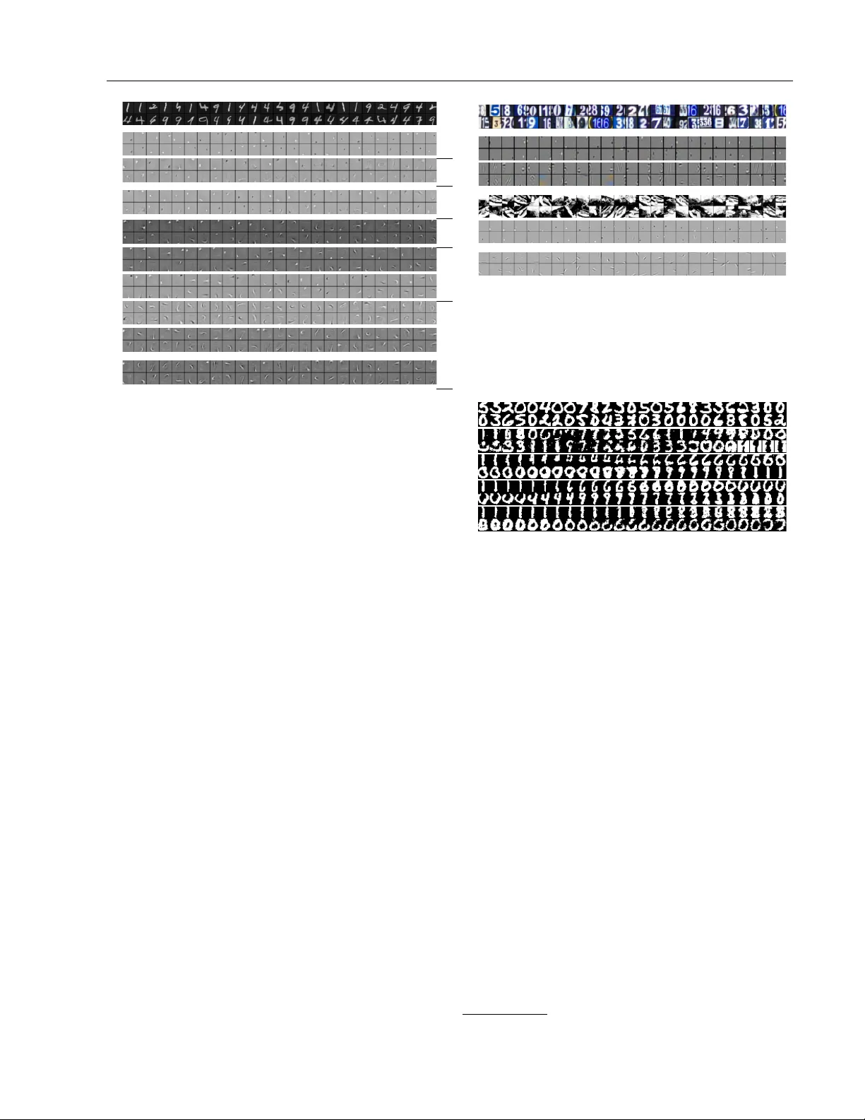
Sto c hastic Neural Net w orks with Monotonic Activ ation F unctions Siamak Ra v an bakhsh, Barnab´ as P´ oczos, Jeff Sc hneider 1 and Dale Sc huurmans, Russell Greiner 2 1 Carnegie Mellon Univ ersity , 5000 F orb es Av e, Pittsburgh, P A 15213 2 Univ ersity of Alberta, Edmonton, AB T6G 2E8, Canada Abstract W e prop ose a Laplace approximation that creates a sto c hastic unit from an y smo oth monotonic activ ation function, using only Gaussian noise. This pap er in vestigates the application of this sto c hastic approximation in training a family of Restricted Boltzmann Mac hines (RBM) that are closely link ed to Bregman divergences. This family , that w e call exp onen tial family RBM (Exp-RBM), is a subset of the exp onen tial family Harmoni- ums that expresses family members through a choice of smo oth monotonic non-linearity for eac h neuron. Using con trastive div ergence along with our Gaussian appro ximation, we sho w that Exp-RBM can learn useful repre- sen tations using nov el sto c hastic units. 1 In tro duction Deep neural netw orks ( LeCun et al. , 2015 ; Bengio , 2009 ) hav e pro duced some of the b est results in complex pattern recognition tasks where the train- ing data is abundant. Here, w e are interested in deep learning for generative modeling. Recen t years has witnessed a surge of in terest in directed gen- erativ e mo dels that are trained using (sto c hastic) bac k-propagation ( e.g. , Kingma and W elling , 2013 ; Rezende et al. , 2014 ; Goo dfello w et al. , 2014 ). These mo dels are distinct from deep energy-based mo d- els – including deep Boltzmann machine ( Hinton et al. , 2006 ) and (conv olutional) deep belief netw ork Appearing in Proceedings of the 19th International Conference on Artificial Intelligence and Statistics (AIST A TS) 2016, Cadiz, Spain. JMLR: W&CP volume 41. Copyright 2016 by the authors ( Salakh utdinov and Hin ton , 2009 ; Lee et al. , 2009 ) – that rely on a bipartite graphical mo del called re- stricted Boltzmann mac hine (RBM) in eac h la yer. Al- though, due to their use of Gaussian noise, the stochas- tic units that we introduce in this pap er can b e p o- ten tially used with sto chastic bac k-propagation, this pap er is limited to applications in RBM. T o this day , the choice of stochastic units in RBM has b een constrained to well-kno wn mem b ers of the exp o- nen tial family; in the past RBMs ha ve used units with Bernoulli ( Smolensky , 1986 ), Gaussian ( F reund and Haussler , 1994 ; Marks and Mov ellan , 2001 ), categori- cal ( W elling et al. , 2004 ), Gamma ( W elling et al. , 2002 ) and P oisson ( Gehler et al. , 2006 ) conditional distribu- tions. The exception to this sp ecialization, is the Rec- tified Linear Unit that was in tro duced with a (heuris- tic) sampling pro cedure ( Nair and Hinton , 2010 ). This limitation of RBM to well-kno wn exp onen tial family members is despite the fact that W elling et al. ( 2004 ) introduced a generalization of RBMs, called Ex- p onen tial F amily Harmoniums (EFH), co vering a large subset of exp onen tial family with bipartite structure. The architecture of EFH does not suggest a proce- dure connecting the EFH to arbitr ary non-line arities and more imp ortantly a general sampling pro cedure is missing. 1 W e introduce a useful subset of the EFH, whic h we call exp onen tial family RBMs (Exp-RBMs), with an approximate sampling pro cedure addressing these shortcomings. The basic idea in Exp-RBM is simple: restrict the sufficien t statistics to iden tity function. This allows definition of each unit using only its mean sto c hastic activ ation, which is the non-linearit y of the neuron. With this restriction, not only w e gain interpretabil- it y , but also trainability; we show that it is p ossible to efficiently sample the activ ation of these sto c has- 1 As the concluding remarks of W elling et al. ( 2004 ) suggest, this capabilit y is indeed desirable:“A future chal- lenge is therefore to start the mo delling pro cess with the desired non-linearit y and to subsequently in troduce auxil- iary v ariables to facilitate inference and learning.” 1 tic neurons and train the resulting mo del using con- trastiv e divergence. In terestingly , this restriction also closely relates the generative training of Exp-RBM to discriminativ e training using the matching loss and its regularization by noise injection. In the following, Section 2 introduces the Exp-RBM family and Section 3 inv estigates learning of Exp- RBMs via an efficient approximate sampling proce- dure. Here, we also establish connections to dis- criminativ e training and produce an in terpretation of sto c hastic units in Exp-RBMs as an infinite collection of Bernoulli units with differen t activ ation biases. Sec- tion 4 demonstrates the effectiv eness of the prop osed sampling pro cedure, when combined with contrastiv e div ergence training, in data representation. 2 The Mo del The conv en tional RBM mo dels the joint probability p ( v , h | W ) for visible v ariables v = [ v 1 , . . . , v i , . . . , v I ] with v ∈ V 1 × . . . × V I and hidden v ariables h = [ h 1 , . . . , h j , . . . h J ] with h ∈ H 1 × . . . × H J as p ( v , h | W ) = exp( − E ( v , h ) − A ( W )) . This join t probabilit y is a Boltzmann distribution with a particular energy function E : V × H → R and a normalization function A . The distinguishing prop ert y of RBM compared to other Boltzmann distributions is the conditional indep endence due to its bipartite structure. W elling et al. ( 2004 ) construct Exp onen tial F amily Harmoniums (EFH), b y first constructing independent distribution ov er individual v ariables: considering a hidden v ariable h j , its sufficient statistics { t b } b and canonical parameters { ˜ η j,b } b , this indep enden t distri- bution is p ( h j ) = r ( h j ) exp  X b ˜ η j,b t b ( h j ) − A ( { ˜ η j,b } b )  where r : H j → R is the b ase me asur e and A ( { η i,a } a ) is the normalization constant. Here, for notational con- v enience, we are assuming functions with distinct in- puts are distinct – i.e. , t b ( h j ) is not necessarily the same function as t b ( h j 0 ), for j 0 6 = j . The authors then com bine these indep enden t distribu- tions using quadratic terms that reflect the bipartite structure of the EFH to get its joint form p ( v , h ) ∝ exp  X i,a ˜ ν i,a t a ( v i ) (1) + X j,b ˜ η j,b t b ( h j ) + X i,a,j,b W a,b i,j t a ( v i ) t b ( h j )  where the normalization function is ignored and the base measures are represen ted as additional sufficient statistics with fixed parameters. In this mo del, the conditional distributions are p ( v i | h ) = exp  X a ν i,a t a ( v j ) − A ( { ν i,a } a  p ( h j | v ) = exp  X b η j,b t b ( h j ) − A ( { η j,b } b  where the shifte d parameters η j,b = ˜ η j,b + P i,a W a,b i,j t a ( v i ) and ν i,a = ˜ ν i,a + P j,b W a,b i,j t b ( h j ) in- corp orate the effect of evidence in netw ork on the ran- dom v ariable of interest. It is generally not p ossible to efficien tly sample these conditionals (or the joint probabilit y) for arbitrary suf- ficien t statistics. More imp ortan tly , the join t form of eq. ( 1 ) and its energy function are “obscure”. This is in the sense that the base measures { r } , dep end on the c hoice of sufficient statistics and the normaliza- tion function A ( W ). In fact for a fixed set of suffi- cien t statistics { t a ( v i ) } i , { t b ( h j ) } j , different compati- ble c hoices of normalization constants and base mea- sures ma y produce diverse subsets of the exp onen tial family . Exp-RBM is one suc h family , where sufficien t statistics are identit y functions. 2.1 Bregman Divergences and Exp-RBM Exp-RBM restricts the sufficient statistics t a ( v i ) and t b ( h j ) to single iden tity functions v i , h j for all i and j . This means the RBM has a single weigh t matrix W ∈ R I × J . As b efore, eac h hidden unit j , receiv es an input η j = P i W i,j v i and similarly each visible unit i receiv es the input ν i = P j W i,j h j . 2 Here, the conditional distributions p ( v i | ν i ) and p ( h j | η j ) hav e a single me an p ar ameter , f ( η ) ∈ M , which is equal to the mean of the conditional distribution. W e could freely assign any desired contin uous and mono- tonic non-linearit y f : R → M ⊆ R to represent the mapping from canonical parameter η j to this mean pa- rameter: f ( η j ) = R H j h j p ( h j | η j ) d h j . This choice of f defines the conditionals p ( h j | η j ) = exp  − D f ( η j k h j ) − g ( h j )  (2) p ( v i | ν i ) = exp  − D f ( ν i k v i ) − g ( v i )  where g is the base measure and D f is the Bregman div ergence for the function f . 2 Note that we ignore the “bias parameters” ˜ ν i and ˜ η j , since they can b e encoded using the w eights for additional hidden or visible units ( h j = 1 , v i = 1) that are clamped to one. unit name non-linearity f ( η ) Gaussian approximation conditional dist p ( h | η ) Sigmoid (Bernoulli) Unit (1 + e − η ) − 1 - exp { η h − log(1 + exp( η )) } Noisy T anh Unit (1 + e − η ) − 1 − 1 2 N ( f ( η ) , ( f ( η ) − 1 / 2)( f ( η ) + 1 / 2)) exp { η h − log(1 + exp( η )) + ent( h ) − g ( h ) } ArcSinh Unit log( η + p 1 + η 2 ) N (sinh − 1 ( η ) , ( p 1 + η 2 ) − 1 ) exp { η h − cosh( h ) + p 1 + η 2 − η sin − 1 ( η ) − g ( h ) } Symmetric Sqrt Unit (SymSqU) sign( η ) p | η | N ( f ( η ) , p | η | / 2) exp { η h − | h | 3 / 3 − 2( η 2 ) 3 4 / 3 − g ( h ) } Linear (Gaussian) Unit η N ( η , 1) exp { η h − 1 2 ( η 2 ) − 1 2 ( h 2 ) − log ( √ 2 π ) } Softplus Unit log(1 + e η ) N ( f ( η ) , (1 + e − η ) − 1 ) exp { η h + Li 2 ( − e η ) + Li 2 ( e h ) + h log(1 − e h ) − h log( e h − 1) − g ( h ) } Rectified Linear Unit (ReLU) max(0 , η ) N ( f ( η ) , I ( η > 0)) - Rectified Quadratic Unit (ReQU) max(0 , η | η | ) N ( f ( η ) , I ( η > 0) η ) - Symmetric Quadratic Unit (SymQU) η | η | N ( η | η | , | η | ) exp { η h − | η | 3 / 3 − 2( h 2 ) 3 4 / 3 − g ( h ) } Exponential Unit e η N ( e η , e η ) exp { η h − e η − h (log( y ) − 1) − g ( h ) } Sinh Unit 1 2 ( e η − e − η ) N (sinh( η ) , cosh( η )) exp { η h − cosh( η ) + √ 1 + h 2 − h sin − 1 ( h ) − g ( h ) } Poisson Unit e η - exp { η h − e η − h ! } T able 1: Sto chastic units, their c onditional distribution (e q. ( 2 ) ) and the Gaussian appr oximation to this distribution. Her e Li( · ) is the polylo garithmic function and I (cond . ) is e qual to one if the c ondition is satisfie d and zer o otherwise. en t( p ) is the binary entr opy function. The Bregman div ergence ( Bregman , 1967 ; Banerjee et al. , 2005 ) b et w een h j and η j for a monotonically increasing transfer function (corresp onding to the ac- tiv ation function) f is given by 3 D f ( η j k h j ) = − η j h j + F ( η j ) + F ∗ ( h j ) (3) where F with d d η F ( η j ) = f ( η j ) is the an ti-deriv ative of f and F ∗ is the an ti-deriv ative of f − 1 . Substitut- ing this expression for Bregmann div ergence in eq. ( 2 ), w e notice b oth F ∗ and g are functions of h j . In fact, these tw o functions are often not separated ( e.g. , Mc- Cullagh et al. , 1989 ). By separating them we see that some times, g simplifies to a constant, enabling us to appro ximate Equation ( 2 ) in Section 3.1 . Example 2.1. Let f ( η j ) = η j b e a linear neu- ron. Then F ( η j ) = 1 2 η 2 j and F ∗ ( h j ) = 1 2 h 2 j , giving a Gaussian conditional distribution p ( h j | η j ) = e − 1 2 ( h j − η j ) 2 + g ( h j ) , where g ( h j ) = log( √ 2 π ) is a con- stan t. 2.2 The Joint F orm So far we hav e defined the conditional distribution of our Exp-RBM as members of, using a single mean pa- rameter f ( η j ) (or f ( ν i ) for visible units) that repre- sen ts the activ ation function of the neuron. Now we 3 The con ven tional form of Bregman div ergence is D f ( η j k h j ) = F ( η j ) − F ( f − 1 ( h j )) − h j ( η j − f − 1 ( h j )), where F is the anti-deriv ativ e of f . Since F is strictly con vex and differen tiable, it has a Legendre-F ench el dual F ∗ ( h j ) = sup η j h h j , η j i − F ( η j ). No w, set the deriv a- tiv e of the r.h.s. w.r.t. η j to zero to get h j = f ( η j ), or η j = f − 1 ( h j ), where F ∗ ( h j ) is the anti-deriv ativ e of f − 1 ( h i ). Using the duality to switch f and f − 1 in the ab o v e we can get F ( f − 1 ( h j )) = h j f − 1 ( h j ) − F ∗ ( h j ). By replacing this in the original form of Bregman divergence w e get the alternative form of Equation ( 3 ). w ould lik e to find the corresponding joint form and the energy function. The problem of relating the lo cal conditionals to the join t form in graphical mo dels go es back to the work of Besag ( 1974 ).It is easy to chec k that, using the more general treatment of Y ang et al. ( 2012 ), the joint form corresp onding to the conditional of eq. ( 2 ) is p ( v , h | W ) = exp  v T · W · h (4) − X i  F ∗ ( v i ) + g ( v i )  − X j  F ∗ ( h j ) + g ( h j )  − A ( W )  where A ( W ) is the join t normalization constan t. It is noteworth y that only the an ti-deriv ative of f − 1 , F ∗ app ears in the join t form and F is absent. F rom this, the energy function is E ( v , h ) = − v T · W · h (5) + X i  F ∗ ( v i ) + g ( v i )  + X j  F ∗ ( h j ) + g ( h j )  . Example 2.2. F or the sigmoid non-linearity f ( η j ) = 1 1+ e − η j , we hav e F ( η j ) = log(1 + e η j ) and F ∗ ( h j ) = (1 − h j ) log(1 − h j ) + h j log( h j ) is the negativ e entrop y . Since h j ∈ { 0 , 1 } only tak es ex- treme v alues, the negative entrop y F ∗ ( h j ) ev aluates to zero: p ( h j | η j ) = exp  h j η j − log(1 + exp( η j )) − g ( h j )  (6) Separately ev aluating this expression for h j = 0 and h j = 1, sho ws that the ab o ve conditional is a well-defined distribution for g ( h j ) = 0, and in fact it turns out to b e the sigmoid function itself – i.e. , p ( h j = 1 | η j ) = 1 1+ e − η j . When all con- ditionals in the RBM are of the form eq. ( 6 ) – i.e. , for a binary RBM with a sigmoid non-linearit y , since { F ( η j ) } j and { F ( ν i ) } i do not app ear in the join t form eq. ( 4 ) and F ∗ (0) = F ∗ (1) = 0, the join t form has the simple and the familiar form p ( v , h ) = exp  v T · W · h − A ( W )  . 3 Learning A consistent estimator for the parameters W , given observ ations D = { v (1) , . . . , v ( N ) } , is obtained by maximizing the marginal likelihoo d Q n p ( v ( n ) | W ), where the eq. ( 4 ) defines the join t probability p ( v , h ). The gradient of the log-marginal-lik eliho od ∇ W  P n log( p ( v ( n ) | W ))  is 1 N X n E p ( h | v ( n ) ,W ) [ h · ( v ( n ) ) T ] − E p ( h,v | W ) [ h · v T ] (7) where the first exp ectation is w.r.t. the observed data in which p ( h | v ) = Q j p ( h j | v ) and p ( h j | v ) is given b y eq. ( 2 ). The second exp ectation is w.r.t. the mo del of eq. ( 4 ). When discriminativ ely training a neuron f ( P i W i,j v i ) using input output pairs D = { ( v ( n ) , h ( n ) j ) } n , in order to hav e a loss that is con vex in the mo del parame- ters W : j , it is common to use a matching loss for the giv en transfer function f ( Helmbold et al. , 1999 ). This is simply the Bregman divergence D f ( f ( η ( n ) j ) k h ( n ) j ), where η ( n ) j = P i W i,j v ( n ) i . Minimizing this matc h- ing loss corresp onds to maximizing the log-likelihoo d of eq. ( 2 ), and it should not b e surprising that the gradient ∇ W : j  P n D f ( f ( η ( n ) j ) k h ( n ) j )  of this loss w.r.t. W : j = [ W 1 ,j , . . . , W M ,j ] X n f ( η ( n ) j )( v ( n ) ) T − h ( n ) j ( v ( n ) ) T resem bles that of eq. ( 7 ), where f ( η ( n ) j ) ab o ve substi- tutes h j in eq. ( 7 ). Ho wev er, note that in generative training, h j is not simply equal to f ( η j ), but it is sampled from the expo- nen tial family distribution eq. ( 2 ) with the mean f ( η j ) – that is h j = f ( η j ) + noise. This extends the previous observ ations linking the discriminative and generative (or regularized) training – via Gaussian noise injection – to the noise from other members of the exp onen tial family ( e.g. , An , 1996 ; Vincent et al. , 2008 ; Bishop , 1995 ) which in turn relates to the regularizing role of generativ e pretraining of neural netw orks ( Erhan et al. , 2010 ). Our sampling scheme (next s ection) further suggests that when using output Gaussian noise injection for regularization of arbitrary activ ation functions, the v ariance of this noise should b e scaled b y the deriv ativ e of the activ ation function. 3.1 Sampling T o learn the generative mo del, we need to b e able to sample from the distributions that define the exp ec- tations in eq. ( 7 ). Sampling from the joint mo del can also b e reduced to alternating conditional sampling of visible and hidden v ariables ( i.e. , blo ck Gibbs sam- pling). Many metho ds, including contrastiv e diver- gence (CD; Hinton , 2002 ), sto c hastic maximum likeli- ho od (a.k.a. p ersisten t CD Tieleman , 2008 ) and their v ariations ( e.g. , Tieleman and Hin ton , 2009 ; Breuleux et al. , 2011 ) only require this alternating sampling in order to optimize an approximation to the gradient of eq. ( 7 ). Here, we are interested in sampling from p ( h j | η j ) and p ( v i | ν i ) as defined in eq. ( 2 ), which is in gen- eral non-trivial. Ho wev er some members of the exp o- nen tial family hav e relatively efficient sampling pro ce- dures ( Ahrens and Dieter , 1974 ). One of these mem- b ers that we use in our exp erimen ts is the Poisson distribution. Example 3.1. F or a P oisson unit, a P oisson dis- tribution p ( h j | λ ) = λ h j h j ! e − λ (8) represen ts the probabilit y of a neuron firing h j times in a unit of time, giv en its av erage rate is λ . W e can define P oisson units within Exp-RBM using f j ( η j ) = e η j , whic h gives F ( η j ) = e η j and F ∗ ( h j ) = h j (log( h j ) − 1). F or p ( h j | η j ) to be prop- erly normalized, since h j ∈ Z + is a non-negativ e in teger, F ∗ ( h j ) + g ( h j ) = log ( h j !) ≈ F ∗ ( h j ) (using Sterling’s approximation). This gives p ( h j | η j ) = exp  h j η j − e η j − log( h j !)  whic h is identical to dis- tribution of eq. ( 8 ), for λ = e η j . This means, w e can use any av ailable sampling routine for Poisson distribution to learn the parameters for an exp o- nen tial family RBM where some units are Poisson. In Section 4 , we use a mo dified v ersion of Kn uth’s metho d ( Knuth , 1969 ) for Poisson sampling. By making a simplifying assumption, the follo wing Laplace approximation demonstrates how to use Gaus- sian noise to sample from general conditionals in Exp- RBM, for “any” smo oth and monotonic non-linearity . Prop osition 3.1. Assuming a c onstant b ase me asur e g ( h i ) = c , the distribution of p ( h j k η j ) is to the se c ond (a) ArcSinh unit (b) Sinh unit (c) Softplus unit (d) Exp unit Figure 1: Conditional pr ob ability of e q. ( 11 ) for differ ent stochastic units (top r ow) and the Gaussian appr oximation of Pr op osition 3.1 (bottom r ow) for the same unit. Her e the horizontal axis is the input η j = P i W i,j v i and the vertic al axis is the sto chastic activation h j with the intensity p ( h j | η j ) . se e T able 1 for more details on these stochastic units. or der appr oximate d by a Gaussian exp  − D f ( η j k h j ) − c  ≈ N ( h j | f ( η j ) , f 0 ( η j ) ) (9) wher e f 0 ( η j ) = d d η j f ( η j ) is the derivative of the acti- vation function. Pr o of. The mo de (and the mean) of the conditional eq. ( 2 ) for η j is f ( η j ). This is b ecause the Bregman div ergence D f ( η j k h j ) achiev es minim um when h j = f ( η j ). Now, write the T aylor series appro ximation to the target log-probability around its mo de log( p ( ε + f ( η j ) | η j )) = log( − D f ( η j k ε + f ( η j ))) − c = η j f ( η j ) − F ∗ ( f ( η j )) − F ( η j ) + ε ( η j − f − 1 ( f ( η j )) + 1 2 ε 2 ( − 1 f 0 ( η j ) ) + O ( ε 3 ) = η j f ( η j ) − ( η j f ( η j ) − F ( η j )) − F ( η j ) + ε ( η j − η j ) + 1 2 ε 2 ( − 1 f 0 ( η j ) ) + O ( ε 3 ) = − 1 2 ε 2 f 0 ( η j ) + O ( ε 3 ) (10a) (10b) (10c) In eq. ( 10a ) w e used the fact that d d y f − 1 ( y ) = 1 f 0 ( f − 1 ( y )) and in eq. ( 10b ), we used the conjugate du- alit y of F and F ∗ . Note that the final unnormalized log-probabilit y in eq. ( 10c ) is that of a Gaussian, with mean zero and v ariance f 0 ( η j ). Since our T aylor ex- pansion was around f ( η j ), this gives us the approxi- mation of eq. ( 9 ). 3.1.1 Sampling Accuracy T o exactly ev aluate the accuracy of our sampling sc heme, w e need to ev aluate the conditional distribu- tion of eq. ( 2 ). Ho wev er, we are not aw are of any an- alytical or numeric metho d to estimate the base mea- sure g ( h j ). Here, we replace g ( h j ) with ˜ g ( η j ), playing the role of a normalization constan t. W e then ev aluate p ( h j | η j ) ≈ exp  − D f ( η j k h j ) − ˜ g ( η j )  (11) where ˜ g ( η j ) is numerically appro ximated for each η j v alue. Figure 1 compares this densit y against the Gaussian appro ximation p ( h j | η j ) ≈ N ( f ( η j ) , f 0 ( η j ) ). As the figure shows, the densities are very similar. 3.2 Bernoulli Ensemble Interpretation This section gives an interpretation of Exp-RBM in terms of a Bernoulli RBM with an infinite collection of Bernoulli units. Nair and Hinton ( 2010 ) introduce the softplus unit, f ( η j ) = log(1 + e η j ), as an approximation to the rectified linear unit (ReLU) f ( η j ) = max(0 , η j ). T o hav e a probabilistic interpretation for this non- linearit y , the authors represent it as an infinite series of Bernoulli units with shifted bias: log(1 + e η j ) = ∞ X n =1 σ ( η j − n + . 5) (12) where σ ( x ) = 1 1+ e − x is the sigmoid function. This means that the sample y j from a softplus unit is effectively the num b er of active Bernoulli units. The authors then suggest using h j ∼ max(0 , N ( η j , σ ( η j )) to sample from this t yp e of unit. In comparison, our Proposition 3.1 suggests using h j ∼ N (log (1 + e η j ) , σ ( η j )) for softplus and h j ∼ N (max(0 , η j ) , step ( η j )) – where step ( η j ) is the step function – for ReLU. Both of these are very similar to the approximation of ( Nair and Hinton , 2010 ) and we found them to p erform similarly in practice as well. Note that these Gaussian approximations are assum- ing g ( η j ) is constant. How ever, b y numerically ap- - 20 - 10 10 20 2 4 6 8 10 12 Figure 2: Numeric al appr oximation to the inte gr al R H j exp  − D f ( η j k h j )  d h j for the softplus unit f ( η j ) = log(1 + e η j ) , at differ ent η j . pro ximating R H j exp  − D f ( η j k h j )  d h j , for f ( η j ) = log(1 + e η j ), Figure 2 shows that the in tegrals are not the same for different v alues of η j , showing that the base measure g ( h j ) is not constant for ReLU. In spite of this, experimental results for pretraining ReLU units using Gaussian noise suggests the usefulness of this type of approximation. W e can extend this interpretation as a collection of (w eighted) Bernoulli units to any non-linearity f . F or simplicit y , let us assume lim η →−∞ f ( η ) = 0 and lim η → + ∞ f ( η ) = ∞ 4 , and define the following series of Bernoulli units: P ∞ n =0 ασ ( f − 1 ( αn )), where the given parameter α is the weigh t of each unit. Here, we are defining a new Bernoulli unit with a weigh t α for each α unit of change in the v alue of f . Note that the un- derlying idea is similar to that of inv erse transform sampling ( Devroy e , 1986 ). At the limit of α → 0 + w e ha ve f ( η j ) ≈ α ∞ X n =0 σ ( η j − f − 1 ( αn )) (13) that is ˆ h j ∼ p ( h j | η j ) is the weigh ted sum of active Bernoulli units. Figure 4 (a) shows the approximation of this series for the softplus function for decreasing v alues of α . 4 Exp erimen ts and Discussion W e ev aluate the represen tation capabilities of Exp- RBM for differen t sto c hastic units in the following t wo sections. Our initial attempt was to adapt An- nealed Imp ortance Sampling (AIS; Salakhutdino v and Murra y , 2008 ) to Exp-RBMs. Ho w ever, estimation of the imp ortance sampling ratio in AIS for general Exp- RBM prov ed challenging. W e consider t wo alterna- tiv es: 1) for large datasets, Section 4.1 qualitatively 4 The following series and the sigmoid function need to be adjusted dep ending on these limits. F or example, for the case where h j is an tisymmetric and unbounded ( e.g. , f ( η j ) ∈ { sinh( η j ) , sinh − 1 ( η j ) , η j | η j |} ), we need to change the domain of Bernoulli units from { 0 , 1 } to {− . 5 , + . 5 } . This corresponds to changing the sigmoid to h yp erb olic tangent 1 2 tanh( 1 2 η j ). In this case, we also need to change the b ounds for n in the series of eq. ( 13 ) to ±∞ . Figure 3: r e c onstruction of R eLU by as a series of Bernoul li units with shifte d bias. Figure 4: Histo gr am of hidden variable activities on the MNIST test data, for different typ es of units. Units with he avier tails pr o duc e longer str okes in Figur e 5 . Note that the line ar de c ay of activities in the lo g-domain corr esp ond to exp onential de c ay with differ ent exp onential c o efficients. ev aluates the filters learned by v arious units and; 2) Section 4.2 ev aluates Exp-RBMs on a smaller dataset where w e can use indirect sampling likelihoo d to quan- tify the generative qualit y of the mo dels with different activ ation functions. Our ob jective here is to demonstrate that a combi- nation of our sampling scheme with contrastiv e di- v ergence (CD) training can indeed pro duce generative mo dels for a diverse choice of activ ation function. 4.1 Learning Filters In this section, we used CD with a single Gibbs sam- pling step, 1000 hidden units, Gaussian visible units 5 , mini-batc hes and metho d of momen tum, and selected the learning rate from { 10 − 2 , 10 − 3 , 10 − 4 } using recon- struction error at the final ep o c h. The MNIST handwritten digits dataset ( LeCun et al. , 1998 ) is a dataset of 70,000 “size-normalized and cen- tered” binary images. Eac h image is 28 × 28 pixel, and represen ts one of { 0 , 1 , . . . , 9 } digits. See the first row of Figure 5 for few instances from MNIST dataset. F or this dataset we use a momentum of . 9 and train each mo del for 25 ep o c hs. Figure 5 shows the filters of dif- feren t sto c hastic units; see T able 1 for details on differ- en t sto c hastic units. Here, the units are ordered based on the asymptotic b eha vior of the activ ation function 5 Using Gaussian visible units also assumes that the in- put data is normalized to hav e a standard deviation of 1. data N.T anh bounded arcSinh log. SymSq sqrt ReL linear ReQ quadratic SymQ Sinh exponential Exp Poisson Figure 5: Samples fr om the MNIST dataset (first two r ows) and the filters with highest varianc e for different Exp- RBM sto chastic units (two r ows p er unit typ e). F rom top to b ottom the non-line arities gr ow mor e rapidly, also pro- ducing fe atur es that r epr esent longer str okes. f ; see the right margin of the figure. This asymptotic c hange in the activ ation function is also eviden t from the hidden unit activ ation histogram of Figure 4 (b), where the activ ation are produced on the test set us- ing the trained mo del. These tw o figures suggest that transfer functions with faster asymptotic gro wth, hav e a more heavy-tailed distributions of activ ations and longer strok es for the MNIST dataset, also hinting that they may b e prefer- able in learning representation ( e.g. , see Olshausen and Field , 1997 ). How ever, this comes at the cost of train- abilit y . In particular, for all exp onen tial units, due to o ccasionally large gradients, we hav e to reduce the learning rate to 10 − 4 while the Sigmoid/T anh unit re- mains stable for a learning rate of 10 − 2 . Other factors that affect the instability of training for exp onential and quadratic Exp-RBMs are large momentum and small num b er of hidden units. Initialization of the w eights could also play an imp ortan t role, and sparse initialization ( Sutskev er et al. , 2013 ; Martens , 2010 ) and regularization schemes ( Go odfellow et al. , 2013 ) could potentially improv e the training of these mo dels. In all exp eriments, we used uniformly random v alues in [ − . 01 , . 01] for all unit t yp es. In terms of training time, different Exp-RBMs that use the Gaussian noise and/or Sigmoid/T anh units hav e similar computation time on b oth CPU and GPU. Figure 6 (top) shows the receptive fields for the street- view house n umbers (SVHN) ( Netzer et al. , 2011 ) dataset. This dataset contains 600,000 images of digits in natural settings. Each image con tains three RGB dataset SVHN sigmoid ReQU dataset NORB T anh SymQU Figure 6: Samples and the r e c eptive fields of different sto chastic units for fr om the (top thr e e r ows) SVHN dataset and (b ottom thr e e r ows) 48 × 48 (non-ster e o) NORB dataset with jittere d obje cts and cluttere d b ack- gr ound. Sele ction of the r e c eptive fields is b ase d on their varianc e. dataset T anh ReL ReQ Sinh Figure 7: Samples fr om the USPS dataset (first two r ows) and few of the c onse cutive samples gener ate d fr om differ ent Exp-RBMs using r ates-FPCD. v alues for 32 × 32 pixels. Figure 6 (b ottom) sho ws few filters obtained from the jittered-cluttered NORB dataset ( LeCun et al. , 2004 ). NORB dataset contains 291,600 stereo 2 × (108 × 108) images of 50 toys under differen t lighting, angle and bac kgrounds. Here, w e use a sub-sampled 48 × 48 v ariation, and rep ort the features learned by t wo t yp es of neurons. F or learn- ing from these t wo datasets, we increased the momen- tum to . 95 and trained different models using up to 50 ep ochs. 4.2 Generating Samples The USPS dataset ( Hull , 1994 ) is relatively smaller dataset of 9,298, 16 × 16 digits. W e binarized this data and used 90%, 5% and 5% of instances for training, v alidation and test resp ectiv ely; see Figure 7 (first tw o ro ws) for instances from this dataset. W e used T anh activ ation function for the 16 × 16 = 256 visible units of the Exp-RBMs 6 and 500 hidden units of different t yp es: 1) T anh unit; 2) ReLU; 3) ReQU and 4)Sinh unit. 6 T anh unit is similar to the sigmoid/Bernoulli unit, with the difference that it is (anti)symmetric v i ∈ {− . 5 , + . 5 } . 2000 4000 6000 8000 10000 Iteration 110 100 90 80 Log Likelihood Tanh ReLU ReQU Sinh training 2000 4000 6000 8000 10000 Iteration 0.86 0.87 0.88 0.89 0.90 0.91 0.92 optimal beta Tanh ReLU ReQU Sinh Figure 8: Indir e ct Sampling Likeliho o d of the test data (left) and β ∗ for the density estimate (right) at differ ent ep o chs (x-axis) for USPS dataset. W e then trained these mo dels using CD with 10 Gibbs sampling steps. Our choice of CD rather than al- ternativ es that are known to pro duce b etter genera- tiv e mo dels, suc h as Persisten t CD (PCD; Tieleman , 2008 ), fast PCD (FPCD; Tieleman and Hin ton , 2009 ) and (rates-FPCD; Breuleux et al. , 2011 ) is due to practical reasons; these alternatives were unstable for some activ ation functions, while CD w as alwa ys well- b eha v ed. W e ran CD for 10,000 epo c hs with three differen t learning rates { . 05 , . 01 , . 001 } for each mo del. Note that here, we did not use metho d of momentum and mini-batc hes in order to to minimize the num b er of hyper-parameters for our quantitativ e comparison. W e used rates-FPCD 7 to generate 9298 × 90 100 sam- ples from eac h mo del – i.e. , the same num ber as the samples in the training set. W e pro duce these sam- pled datasets ev ery 1000 ep ochs. Figure 7 sho ws the samples generated by different mo dels at their final ep och, for the “b est c hoices” of sampling parameters and learning rate. W e then used these samples D sample = { v (1) , . . . , v ( N =9298) } , from each mo del to esti- mate the Indirect Sampling Likelihoo d (ISL; Breuleux et al. , 2011 ) of the v alidation set. F or this, we built a non-parametric density estimate ˆ p ( v ; β ) = N X n =1 256 Y j =1 β I ( v ( n ) j = v j ) (1 − β ) I ( v ( n ) j 6 = v j ) (14) and optimized the parameter β ∈ ( . 5 , 1) to maxi- mize the lik eliho od of the v alidation set – that is β ∗ = arg β max Q v ∈ D valid ˆ p ( v , β ). Here, β = . 5 defines a uniform distribution ov er all p ossible binary images, while for β = 1, only the training instances hav e a non-zero probability . W e then used the densit y estimate for β ∗ as well as the b est rates-FPCD sampling parameter to ev aluate 7 W e used 10 Gibbs sampling steps for eac h sample, zero deca y of fast weigh ts – as suggested in ( Breuleux et al. , 2011 ) – and three different fast rates { . 01 , . 001 , . 0001 } . the ISL of the test set . At this point, we hav e an estimate of the likelihoo d of test data for eac h hidden unit t yp e, for ev ery 1000 iteration of CD up dates. The lik eliho o d of the test data using the densit y estimate pro duced dir e ctly fr om the tr aining data , gives us an upp er-bound on the ISL of these mo dels. Figure 8 presen ts all these quantities: for each hidden unit t yp e, we present the results for the learning rate that achiev es the highest ISL. The figure shows the es- timated log-likelihoo d (left) as well as β ∗ (righ t) as a function of the n umber of ep o c hs. As the num b er of iterations increases, all models pro duce samples that are more representativ e (and closer to the training-set lik eliho o d). This is also consisten t with β ∗ v alues get- ting closer to β ∗ training = . 93, the optimal parameter for the training set. In general, we found sto c hastic units defined using ReLU and Sigmoid/T anh to b e the most numerically stable. Ho w ever, for this problem, ReQU learns the b est mo del and even by increasing the CD steps to 25 and also increasing the ep o c hs by a factor of tw o w e could not produce similar results using T anh units. This shows that a non-linearities outside the circle of well-kno wn and commonly used exp onen tial fam- ily , can sometimes pro duce more pow erful generative mo dels, even using an “approximate” sampling pro ce- dure. Conclusion This pap er studies a subset of exp onen tial family Har- moniums (EFH) with a single sufficien t statistics for the purp ose of learning generativ e mo dels. The result- ing family of distributions, Exp-RBM, gives a freedom of choice for the activ ation function of individual units, paralleling the freedom in discriminative training of neural netw orks. Moreov er, it is p ossible to efficiently train arbitrary members of this family . F or this, we in tro duced a principled and efficien t appro ximate sam- pling pro cedure and demonstrated that v arious Exp- RBMs can learn useful generative mo dels and filters. References Joac him H Ahrens and Ulric h Dieter. Computer meth- o ds for sampling from gamma, b eta, p oisson and bionomial distributions. Computing , 12(3):223–246, 1974. Guozhong An. The effects of adding noise during bac kpropagation training on a generalization p er- formance. Neur al Computation , 8(3):643–674, 1996. Arindam Banerjee, Srujana Merugu, Inderjit S Dhillon, and Joydeep Ghosh. Clustering with breg- man divergences. JMLR , 6:1705–1749, 2005. Y oshua Bengio. Learning deep architectures for ai. F oundations and tr ends in ML , 2(1), 2009. Julian Besag. Spatial interaction and the statistical analysis of lattice systems. Journal of the R oyal Statistic al So ciety. Series B (Metho dolo gic al) , pages 192–236, 1974. Chris M Bishop. T raining with noise is equiv alent to tikhono v regularization. Neur al c omputation , 7(1): 108–116, 1995. Lev M Bregman. The relaxation metho d of finding the common p oin t of conv ex sets and its application to the solution of problems in conv ex programming. USSR CMMP , 7(3):200–217, 1967. Olivier Breuleux, Y oshua Bengio, and Pascal Vincent. Quic kly generating represen tative samples from an rbm-deriv ed process. Neur al Computation , 23(8): 2058–2073, 2011. L. Devroy e. Non-uniform r andom variate gener ation . Springer-V erlag, 1986. ISBN 9783540963059. Dumitru Erhan, Y osh ua Bengio, Aaron Courville, Pierre-An toine Manzagol, P ascal Vincent, and Samy Bengio. Why do es unsup ervised pre-training help deep learning? JMLR , 11:625–660, 2010. Y oav F reund and David Haussler. Unsup ervise d le arn- ing of distributions of binary ve ctors using two layer networks . Computer Researc h Laboratory [Univ er- sit y of California, Santa Cruz], 1994. P eter V Gehler, Alex D Holub, and Max W elling. The rate adapting poisson mo del for information re- triev al and ob ject recognition. In Pr o c e e dings of the 23r d international c onfer enc e on Machine le arning , pages 337–344. ACM, 2006. Ian Go o dfello w, Jean P ouget-Abadie, Mehdi Mirza, Bing Xu, David W arde-F arley , Sherjil Ozair, Aaron Courville, and Y oshua Bengio. Generative adv ersar- ial nets. In A dvanc es in Neur al Information Pr o c ess- ing Systems , pages 2672–2680, 2014. Ian J Go odfellow, David W arde-F arley , Mehdi Mirza, Aaron Courville, and Y osh ua Bengio. Maxout net- w orks. arXiv pr eprint arXiv:1302.4389 , 2013. Da vid P Helmbold, Jyrki Kivinen, and Manfred K W armuth. Relativ e loss bounds for single neu- rons. Neur al Networks, IEEE T r ansactions on , 10 (6):1291–1304, 1999. Geoffrey Hin ton. T raining pro ducts of experts by min- imizing contrastiv e div ergence. Neur al c omputation , 14(8):1771–1800, 2002. Geoffrey Hinton, Simon Osindero, and Y ee-Wh y e T eh. A fast l earning algorithm for deep b elief nets. Neur al c omputation , 18(7):1527–1554, 2006. Jonathan J Hull. A database for handwritten text recognition research. Pattern Analysis and Machine Intel ligenc e, IEEE T r ansactions on , 16(5):550–554, 1994. Diederik P Kingma and Max W elling. Auto-enco ding v ariational ba yes. arXiv pr eprint arXiv:1312.6114 , 2013. Donald E Knuth. Semin umerical algorithms. the art of computer programming, 1969. Y ann LeCun, L´ eon Bottou, Y oshua Bengio, and P atrick Haffner. Gradient-based learning applied to do cumen t recognition. Pr o c e e dings of the IEEE , 86 (11):2278–2324, 1998. Y ann LeCun, F u Jie Huang, and Leon Bottou. Learn- ing metho ds for generic ob ject recognition with in- v ariance to p ose and lighting. In CVPR, 2004 , vol- ume 2, pages I I–97, 2004. Y ann LeCun, Y oshua Bengio, and Geoffrey Hin ton. Deep learning. Natur e , 521(7553):436–444, 2015. Honglak Lee, Roger Grosse, Ra jesh Ranganath, and Andrew Y Ng. Conv olutional deep belief netw orks for scalable unsup ervised learning of hierarchical represen tations. In Pr o c e e dings of the 26th A n- nual International Confer enc e on Machine L e arn- ing , pages 609–616. ACM, 2009. Tim K Marks and Ja vier R Mo vellan. Diffusion net- w orks, pro duct of exp erts, and factor analysis. In Pr o c. Int. Conf. on Indep endent Comp onent Analy- sis , pages 481–485, 2001. James Martens. Deep learning via hessian-free opti- mization. In ICML-10 , pages 735–742, 2010. P eter McCullagh, John A Nelder, and P McCullagh. Gener alize d line ar mo dels , volume 2. Chapman and Hall London, 1989. Vino d Nair and Geoffrey E Hinton. Rectified linear units improv e restricted b oltzmann machines. In ICML-10 , pages 807–814, 2010. Y uv al Netzer, T ao W ang, Adam Coates, Alessandro Bissacco, Bo W u, and Andrew Y Ng. Reading digits in natural images with unsup ervised feature learning. In NIPS workshop , v olume 2011, page 5. Granada, Spain, 2011. Bruno A Olshausen and David J Field. Sparse co ding with an ov ercomplete basis set: A strategy employ ed b y v1? Vision r ese ar ch , 37(23):3311–3325, 1997. Danilo Jimenez Rezende, Shakir Mohamed, and Daan Wierstra. Sto c hastic backpropagation and approx- imate inference in deep generativ e mo dels. arXiv pr eprint arXiv:1401.4082 , 2014. Ruslan Salakh utdinov and Geoffrey E Hin ton. Deep b oltzmann machines. In International Confer enc e on Artificial Intel ligenc e and Statistics , pages 448– 455, 2009. Ruslan Salakhutdino v and Iain Murray . On the quanti- tativ e analysis of deep b elief net works. In ICML-08 , pages 872–879. ACM, 2008. P aul Smolensky . Information pro cessing in dynamical systems: F oundations of harmon y theory . 1986. Ily a Sutskev er, James Martens, George Dahl, and Ge- offrey Hin ton. On the imp ortance of initialization and momentum in deep learning. In ICML-13 , pages 1139–1147, 2013. Tijmen Tieleman. T raining restricted b oltzmann ma- c hines using approximations to the likelihoo d gradi- en t. In Pr o c e e dings of the 25th international c onfer- enc e on Machine le arning , pages 1064–1071. ACM, 2008. Tijmen Tieleman and Geoffrey Hinton. Using fast w eights to improv e persistent contrastiv e diver- gence. In Pr o c e e dings of the 26th A nnual Inter- national Confer enc e on Machine L e arning , pages 1033–1040. ACM, 2009. P ascal Vincent, Hugo Laro c helle, Y oshua Bengio, and Pierre-An toine Manzagol. Extracting and compos- ing robust features with denoising auto enco ders. In ICML-08 , pages 1096–1103, 2008. Max W elling, Simon Osindero, and Geoffrey E Hinton. Learning sparse top ographic representations with pro ducts of student-t distributions. In A dvanc es in neur al information pr o c essing systems , pages 1359– 1366, 2002. Max W elling, Michal Rosen-Zvi, and Geoffrey E Hin- ton. Exp onen tial family harmoniums with an ap- plication to information retriev al. In NIPS , pages 1481–1488, 2004. Eunho Y ang, Genevera Allen, Zhandong Liu, and Pradeep K Ra vikumar. Graphical mo dels via gen- eralized linear mo dels. In NIPS , pages 1358–1366, 2012. Algorithm 1: T raining Exp-RBMs using contrastiv e div ergence Input : training data D = { v ( n ) } 1 ≤ n ≤ N ;#CD steps; #ep ochs; learning rate λ ; activ ation functions { f ( v i ) } i , { f ( h j ) } j Output : mo del parameters W Initialize W for #ep o chs do /* positive phase (+) */ + η ( n ) j = P i W i,j + v ( n ) i ∀ j, n if using Gaussian apprx. then + h ( n ) j ∼ N ( f ( + η ( n ) j ) , f 0 ( + η ( n ) j )) ∀ j, n else + h ( n ) j ∼ p ( h j | + v ( n ) ) ∀ j, n − h ( n ) ← + h ( n ) ∀ n /* negative phase (-) */ for #CD steps do − ν ( n ) i = P j W i,j − h ( n ) i ∀ i, n if using Gaussian apprx. then − v ( n ) i ∼ N ( f ( − ν ( n ) i ) , f 0 ( − ν ( n ) i )) ∀ i, n else − v ( n ) j ∼ p ( v j | h ( n ) ) ∀ i, n − η ( n ) j = P i W i,j − v ( n ) i ∀ j, n if using Gaussian apprx. then − h ( n ) j ∼ N ( f ( − η ( n ) j ) , f 0 ( − η ( n ) j )) ∀ j, n else + h ( n ) j ∼ p ( h j | − v ( n ) ) ∀ j, n end W i,j ← W i,j + λ  ( + v i + h j ) − ( − v i − h j )  ∀ i, j end