On the Modeling of Error Functions as High Dimensional Landscapes for Weight Initialization in Learning Networks

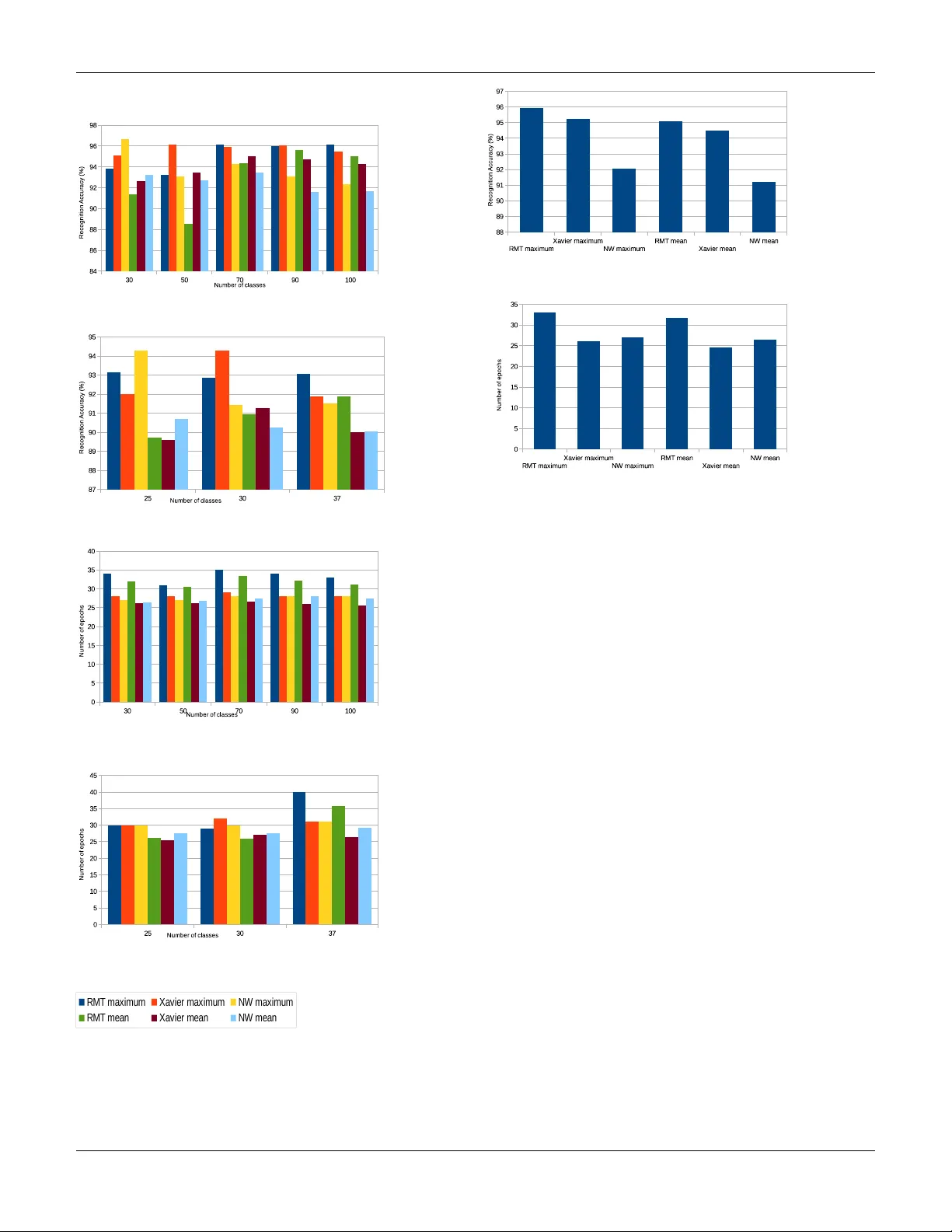
On the Modeling of Error Functions as High Dimensional Landscapes for W eight Initialization in Learning Networks Julius 1 , Gopinath Mahale 2 , Sumana T . 2 , C. S. Adityakrishna 3 { 1 Department of Physics, 3 Department of Computer Science } , BITS-Pilani Hyderabad, India, 2 CAD Lab, Indian Institute of Science, India Email: { juliuswombat,aditya.chivukula } @gmail.com { mahale gv , sumana.t } @cadl.iisc.ernet.in Abstract —Next generation deep neural networks f or classifica- tion hosted on embedded platforms will rely on fast, efficient, and accurate lear ning algorithms. Initialization of weights in learning networks has a gr eat impact on the classification accuracy . In this paper we f ocus on deriving good initial weights by modeling the error function of a deep neural network as a high-dimensional landscape. W e observe that due to the inherent complexity in its algebraic structure, such an error function may conform to general results of the statistics of large systems. T o this end we apply some results fr om Random Matrix Theory to analyse these functions. W e model the error function in terms of a Hamiltonian in N-dimensions and derive some theoretical results about its general beha vior . These r esults are further used to make better initial guesses of weights for the learning algorithm. I . I N T RO D U C T I O N Machine learning is a discipline in which correlations drawn from samples are used in adaptiv e algorithms to extract critical and relev ant information that helps in classification. The interplay between the formulations of learning models in the primal/dual spaces has a great impact in the theoretical analysis and in the practical implementation of the system, more so when emerging embedded platforms play host to a variety of classification systems and applications. Clearly , the demand on performance ef ficiency and accurac y of such machine learning system is of paramount interest. Learning can be supervised, unsupervised or even a combi- nation of the two. In face recognition systems for instance, machine learning is typically supervised since it is trained using a sample set of faces. Whereas, in big data analytics, machine learning is unsupervised since there is no a priori knowledge of the features/information associated with the data. In the terminology of machine learning classification is considered an instance of supervised learning, i.e. learning where a training set of correctly identified observations is av ailable (i.e. the training set is labelled). In unsupervised learning, a model is prepared by deducing structures present in the input data (which is either not labelled or no a priori labelling is known) and project them as general rules. This could mean identifying a mathematical method/process for data organization that systematically reduces redundancy . The corresponding unsupervised procedure is kno wn as clustering, and in volves grouping data into categories based on some measure of inherent similarity or distance. In semi-supervised learning, input data is a mixture of labelled and unlabelled samples. There is a desired prediction problem but the model must learn the structures to organize the data as well as mak e predictions. Neural netw orks (NNs) are one of the major dev elopments in the field of machine learning. The popularity of NNs is due to its substantial learning capacity and adaptability to v arious application domains. The building blocks of a NN are called neurons that act as processing nodes. Such nodes arranged in layers make the network. The layers are called input, hidden or output layer based on their function and visibility to the programmer . These layers are interconnected by synaptic links that hav e associated synaptic weights. A pictorial representa- tion of a neuron and a feed forward neural network is shown in Fig. 1(a) and Fig. 1(b) respecti vely . Training a NN refers to tuning the synaptic weights to implement a giv en function. The function computed by each neuron is y = f w b + N X i =1 w i × x i ! (1) where, N is the dimension of the input sample. x i and w i are i th element of the input sample and weight vector respectiv ely . w b is weight associated with the bias input as shown in Fig. 1(a). f is a differentiable non-linear function. Some of the popular non-linear functions used are sigmoid , tanh , ReLU etc. During training of this neuron, samples x tr from the training database X tr , each associated with labels y tr are used to train the synaptic weights. This tuning of weights is performed to minimize the error function which is a function of difference between the predicted output and the actual output gi ven by E = 1 N samp × N samp X i =1   y tr i − f   w b + N X j =1 w j × x tr i,j     2 (2) where x tr i,j is the j th element of i th training sample and N samp is the number of training samples. The error function is a high dimensional landscape, which needs to be explored for its minima. A single neuron can be trained using standard procedures such as gradient descent that updates the weights based on In the proceedings of the 16th International Conference on Embedded Computer Systems: Architectures, MOdeling, and Simulation (SAMOS) 2016 gradient of the error function. When it comes to the training of a multi-layer feed forward NN, the gradient descent inv olves layer-wise computation of gradients and tuning the weights accordingly . This method is popularly known as the Back propagation. T o train a multi-layer NN using back propagation, there are two main design parameters to be chosen. First, the learning rate which can be visualized as a step size in the search for minima in the error landscape. During training, dynamic update of learning rate has sho wn to perform better learning in practical examples. The second, but more important, design parameter to be chosen is the initial synaptic weights to start the back propagation. The initialized weights hav e shown to af fect the number of iterations required for the con vergence along with the classification performance of the trained network [1]. W eight initialization methods such Xavier method [2] and Nguyen-W idrow method [3] are being used in deep learning frame works like Caf fe [4] and Matlab Neural Network T oolbox [5] for faster and efficient learning. Majority of these deep learning frame works employ stochastic gradient descent algorithms to arriv e at the optimal weight vector for accurate classification. Deep Neural Networks (DNNs) [6] hav e recently emerged as the area of interest for researchers in the field of machine learning. The strength of DNN lies in the multiple layers of neurons that together are capable of representing a lar ge set of complex functions. Although we see numerous applications of DNN, training DNNs has always been a challenge due to the large number of layers. In addition, these very deep networks hav e witnessed the problem of vanishing gradients [7], that has encouraged the researchers to e xplore better methods of initializations. A good weight initialization has shown to play a crucial role in achieving better minima with faster learning in DNNs. Therefore, there is a need for better weight initialization methods that will play a major role in training emer ging very deep neural networks. In this paper we explore statistical methods from Random Matrix Theory (RMT) [8] for large systems, and apply these concepts to explore High Dimensional Landscapes of Error Functions for fast learning. While such methods hav e been applied to problems in Physics to study complex energy lev els of heavy nuclei, financial analytics for stock correlations, com- f 1 w b x 1 x 2 x N w 1 w 2 w N Ʃ (a) A single neuron 1 Inpu t V ect or Inpu t La y er Hid den La y er Outp ut La y er Decis ion Bias Inpu t w y 1 Bias Inpu t w (b) A three layer feed forward neural network Fig. 1. A single neuron and a feed forward neural network munication theory of wireless systems, array signal processing, this is for the first time (to the best of our kno wledge) that such a method is being applied to learning systems. The rest of the paper is organized as follows. In section II we giv e a brief introduction to the RMT and its applicability in learning systems in the context of prior work. W e refer to analysis of RMT and results in the literature which are the basis for dev elopment of our approach for faster learning. In section III, we describe our approach that applies RMT to the problem of learning in neural netw orks. Section IV contains analysis of different parameters in RMT to improve the learning ability of the network along with related results to support our theory . W e conclude in section V. I I . S O M E H I S T O RY : R A N D O M M A T R I X T H E O RY A N D R E L A T E D W O R K Lately Random Matrix Theory (RMT) has been applied effecti vely in various fields of science and engineering [8]. The fact that little kno wledge of RMT is suf ficient for its application [8] has encouraged considerable research work tow ards exploring applicability of RMT in dif ferent application domains. W e present two fundamental results of RMT that appear again and again in many of the models characterized by random matrices. A. The Semicir cle Law W igner’ s Semicircle Law [9] can be stated as follo ws Consider an ensemble of N × N r eal symmetric matrices with independent identically distributed r andom variables fr om a fixed pr obability distribution p ( x ) with mean 0, variance 1, and other moments finite. Then as N → ∞ µ A,N ( x ) = ( 2 π √ 1 − x 2 if | x | ≤ 1 0 otherwise (3) In other words, the sum of normalized eigen values in an interval [ a, b ] ⊂ [ − 1 , 1] is found by integr ating the semicir cle over that interval. The semicircle law provides the requisite connection be- tween the eigen values of a random matrix and the moments of an ensemble of random matrices. B. The T racy W idom Law Problems regarding the motion of a particle in a high- dimensional landscape occur throughout physics in v arious disciplines such as Spin-glass theory , String theory , the theory of Supercooled liquids, etc. [10]. The dynamics of a system in an N -dimensional potential can be described by dy i dx = −∇ i V (4) where V = V ( x 1 , x 2 , ..., x n ) is the functional form of the potential of interest. A high-dimensional landscape is charac- terized by its stationary points. Stationary points are points on the landscape where a particle moving on it is at equilibrium. At stationary points, the gradient of the potential vanishes. The 2 In the proceedings of the 16th International Conference on Embedded Computer Systems: Architectures, MOdeling, and Simulation (SAMOS) 2016 nature of the stationary points is determined by the laplacian of the potential which is giv en by the eigen values of the Hessian matrix of the system. A matrix element of the Hessian matrix is defined as H ij = ∇ 2 ij V (5) The probability of finding a local minima is gi ven by P ( λ 1 < 0 , λ 2 < 0 , ..., λ n < 0) . This is equiv alent to finding the probability that the maximal eigen value λ max < 0 . The study of the maximal eigenv alue of a random matrix is thus of appreciable interest in disciplines that study high-dimensional landscapes. T racy and W idom [11] showed in 1994 that the distribution of the maximal eigen value of an ensemble of random matrices is given by P ( λ max ≤ w , N ) = F β ( √ 2 N − 2 / 3 ( w − √ 2)) (6) where F β is obtained from the solution to the Painlev ´ e II equation. β = 1 corresponds to the Gaussian Orthogonal Ensemble (G.O.E.). The G.O.E. will be our ensemble of interest in this paper . Setting β = 1 the expression for F 1 (x) is gi ven by F 1 ( x ) = exp  − 1 2 Z ∞ x (( y − x ) q 2 ( y ) + q ( y )) dy  (7) where q is giv en by d 2 y dx 2 = 2 q 3 ( y ) + yq ( y ) (8) Here N is the dimension of the random matrix under con- sideration. The Trac y Widom Law thus provides us with a powerful analytical tool in the study of minima of a large random landscape: the main subject of this paper . C. High Dimensional Landscapes Fyodorov et. al. [12] state that finding total number of stationary points in a spatial domain of random landscape is difficult and no efficient techniques are av ailable to perform the task. Ho wev er , it is possible to perform such calculation for Gaussian fields H ( x ) which hav e isotropic cov ariance structure, i.e., cov ariance only dependent on the Euclidean distances | x 1 − x 2 | . The estimation of stationary points in a spatial domain is equi valent to ev aluating the mean density of eigen values of the Gaussian Orthogonal Ensemble (G.O.E.) of real N × N random matrices which has a well established closed form e xpression [13]. W e refer to concepts in [12] to build a base for our theory elaborated in section III. W e consider a random Gaussian landscape H = µ 2 N X i =1 n 2 i + V ( n 1 , n 2 , ..., n N ) (9) where µ is a tuning parameter and V is a random mean-zero Gaussian-distributed field with cov ariance gi ven by h V ( m ) , V ( n ) i = N f  1 2 N | m − n | 2  (10) where f ( x ) is a smooth function decaying at infinity . Com- paring H ( x ) with the Gaussian Orthogonal Ensemble (G.O.E.) and applying the tools [12] of RMT , one can count the av erage number of minima hN m i of H . As discussed in [12], hN m i is gi ven by hN m i =  µ c µ  N 2 ( N +3) / 2 Γ( N +3 2 ) √ π ( N + 1) N N/ 2 I N  µ µ c  (11) where I N ( µ/µ c ) is gi ven by I N  µ µ c  = Z ∞ −∞ e  s 2 2 − N 2  s √ 2 N − µ µ c  2  d ds ( P N +1 ( λ max ≤ s )) ds (12) Here µ c = p f 00 (0) . P N ( λ max ≤ s ) is the probability that the maximal eigen value of a standardized G.O.E. matrix M is smaller than s . The T racy-W idom Law [11] giv es us the following formula as N → ∞ . P N λ max − √ 2 N N − 1 / 6 / √ 2 ≤ s ! ∼ F 1 ( s ) (13) where F 1 is a special solution of the Painlev ´ e II equation. Substituting back into equation 12 we get I N  µ µ c  = Z ∞ −∞ e h N ( t ) dt (14) where h N ( t ) is h N ( t ) = s 2 t 2 − N 2 s t r 2 N − µ µ c ! 2 + ln F 0 1 ( t ) (15) where s t = p 2( N + 1) + t ( N +1) − 1 / 6 √ 2 . Thus as originally shown in [12] expressions 11, 14 and 15 help to arri ve at the av erage number of minima for the energy landscape defined by H . The explicit formula for P N ( λ max ≤ s ) is P N ( λ max ≤ s ) = Z N ( s ) Z N ( ∞ ) (16) where Z N is Z N ( s ) = Z s −∞ dλ 1 Z s −∞ dλ 2 · · · Z s −∞ dλ N Y i