UBL: an R package for Utility-based Learning

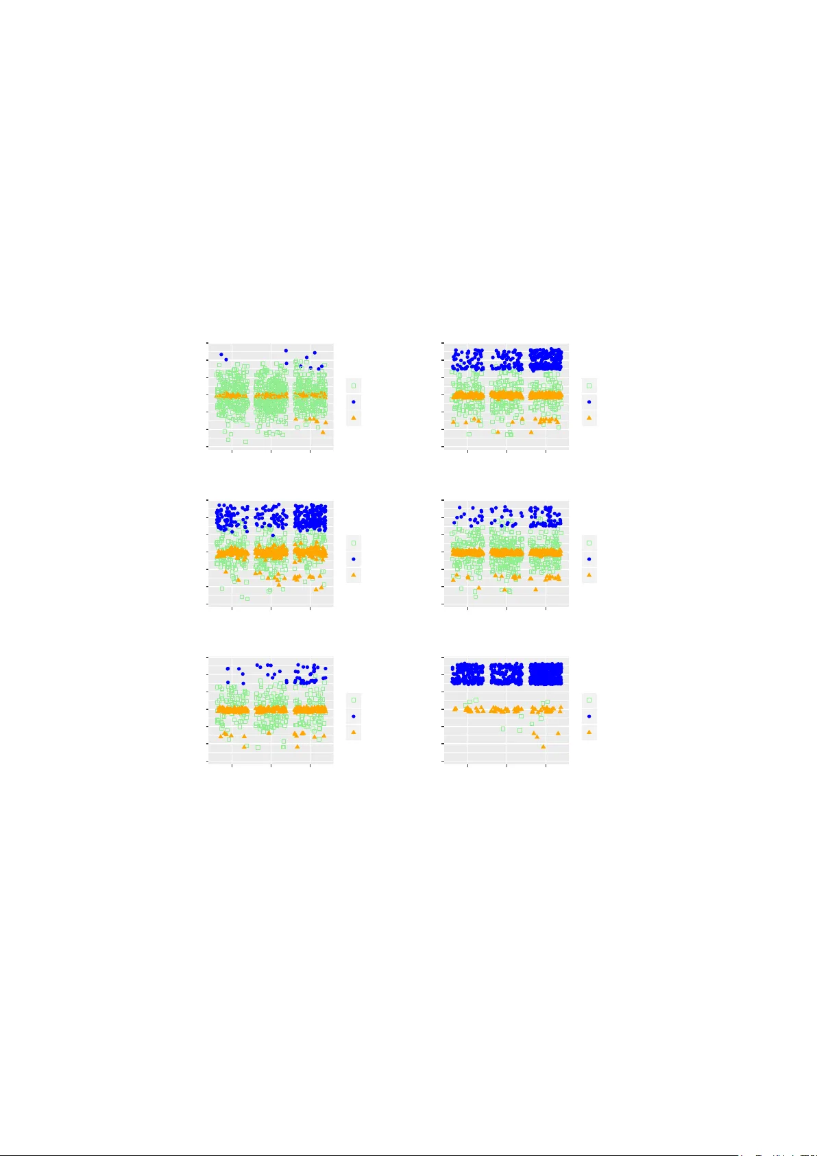
UBL: an R P ac k age for Utilit y-Based Learning P aula Branco, Rita P . Ribeiro and Luis T orgo F CUP - LIAAD/INESC T ec Univ ersity of Porto { paula.branco,rpribeiro,ltorgo } @dcc.fc.up.pt July 14, 2016 Abstract This do cumen t describ es the R pack age UBL that allows the use of sev- eral metho ds for handling utilit y-based learning problems. Classiﬁcation and regression problems that assume non-uniform costs and/or b eneﬁts p ose serious challenges to predictive analytic tasks. In the con text of me- teorology , ﬁnance, medicine, ecology , among many other, speciﬁc domain information concerning the preference bias of the users m ust b e taken in to account to enhance the mo dels predictive p erformance. T o deal with this problem, a large num b er of tec hniques w as proposed by the researc h comm unity for both classiﬁcation and regression tasks. The main goal of UBL pack age is to facilitate the utility-based predictiv e analytic task by pro viding a set of metho ds to deal with this type of problems in the R en vironment. It is a v ersatile to ol that provides mec hanisms to handle b oth regression and classiﬁcation (binary and multiclass) tasks. More- o ver, UBL pac k age allows the user to sp ecify his domain preferences, but it also provides some automatic metho ds that try to infer those preference bias from the domain, considering some common kno wn settings. 1 In tro duction This do cument describes the metho ds a v ailable in pac k age UBL 1 to deal with utilit y-based problems. UBL pack age aims at providing a diverse set of metho ds to address predictive tasks where the user has a non-uniform preference bias across the domain. The pack age pro vides tools suitable for b oth classiﬁcation and regression tasks. All the methods av ailable in UBL pack age w ere extended for b eing able to deal with multiclass problems and with regression problems p ossibly con taining several relev an t regions across the target v ariable domain. Utilit y-based problems are deﬁned in the con text of predictiv e tasks where the user has a diﬀeren tiated in terest o ver the domain. This means that, in this type of problems, the user has non-uniform beneﬁts for the correct predic- tions and/or assumes non-uniform costs for diﬀerent errors. Man y real world applications are utility-based learning problems b ecause they encompass do- main sp eciﬁc information whic h, if disregarded, ma y strongly penalize the per- formance of predictiv e mo dels. This happ ens in the context of meteorology , 1 This document was written for UBL pack age version 0.0.5. 1 ﬁnance, medicine, ecology , among man y other, where sp eciﬁc domain informa- tion concerning the user preferences must b e tak en in to accoun t to enhance the mo dels predictiv e p erformance. In the utilit y-based learning framework w e can frequently witness the con- jugation of tw o imp ortan t factors: i) an increased interest in some particular range(s)/class(es) of the target v ariable v alues and ii) a scarce represen tation of the examples b elonging to that range(s)/class(es). This situation o ccurs in b oth classiﬁcation and regression tasks and is usually kno wn as the problem of im balanced domains [BTR15]. Utilit y-based learning assumes non-uniform costs and/or b eneﬁts which are usually expressed through a cost/b eneﬁt matrix (in classiﬁcation) or a cost/b eneﬁt surface (in regression). Ho wev er, frequen tly this information is just not av ail- able, or is hard/expensive to obtain b ecause it often requires the interv ention of a domain exp ert. This means that for man y domains, there is only an infor- mal kno wledge regarding which are the most costly mistakes and which are the most important classes/ranges of the target v ariable. In fact, considering the particular problem of im balanced classes it is frequent to observ e the assump- tion that “the minority class is the most important one”. This is an imp ortant information regarding the preferences of the user. How ever, it is stated in a v ery informal w ay , an no cost/beneﬁt matrix is av ailable in this situation. The ap- proac hes prop osed in pac k age UBL are able to deal with these situations because they allow the use of b oth user sp eciﬁed preferences and automatic methods. Sev eral types of approac hes exist for handling utilit y-based learning prob- lems. These approaches were categorized in to: pre-pro cessing, change the learn- ing algorithms, p ost-pro cessing or hybrid [BTR15]. The pre-pro cessing ap- proac hes act before the learning stage by manipulating the examples distribution to match the user preferences. The metho ds that change the learning al- gorithms try to incorp orate the user preference bias in to the selected learning algorithm. There are also strategies that are applied as a p ost-pro cessing step b y changing the predictions made by a standard learner using the original data set. Finally there are h ybrid approac hes that combine some of the previous strategies. In pack age UBL w e ha ve fo cused on pre-pro cessing strategies to address the problem of utility-based learning. These strategies change the original distri- bution of examples by removing or/and adding examples, i.e., by p erforming under-sampling or ov er-sampling. The under-sampling strategies may b e ran- dom or fo cused. By fo cused under-sampling we mean that the discarded ex- amples satisfy a giv en requirement, suc h as: are p ossibly noisy examples, are to o distant from the decision b order, are too close to the border, etc. Regard- ing the ov er-sampling metho ds there are t w o main options: ov er-sampling is accomplished b y the introduction of replicas of examples or by the generation of new synthetic examples. F or the strategies which include copies of existing examples, the cases may b e selected randomly or in an informed fashion. Ap- proac hes that build syn thetic cases diﬀer among themselves in the generation pro cess adopted. Sev eral strategies combine under-sampling and ov er-sampling metho ds in diﬀerent ranges/classes of the target v ariable. This do cument is organized as follo ws. In Section 2 some general installa- tion guidelines for UBL pac k age are pro vided. Section 3 brieﬂy describes the t wo syn thetic data sets provided with UBL pac k age . Section 4 presents tw o simple examples to show how UBL pack age can b e used b oth in classiﬁcation and re- 2 gression con texts and its impact on the mo dels p erformance. Sections 5 and 6 describ e with detail each metho d currently implemen ted in UBL for classiﬁca- tion and regression tasks. Section 7 describ es the distance functions a v ailable in pac k age UBL which allow to asses the distance b etw een examples in data sets con taining nominal and/or n umeric features. Finally , Section 8 concludes this do cumen t. 2 P ac k age Installation Guidelines The installation of an y R pack age av ailable on CRAN is p erformed as follows: install.packages ( "UBL" ) This is mandatory , if y ou wan t to use the approaches a v ailable in pack age UBL or even if y ou just wan t to try out the examples presen ted in the next sections. This installs the current stable version of UBL pack age which is version 0.0.5. Y ou may also install the dev elopmen t version of the pac k age, that is av ail- able on the follo wing GitHub W eb page: https://github.com/paobranco/UBL . Ho wev er, w e strongly recommend the use of the CRAN stable v ersion. If y ou still wan t to install the developmen t version, y ou should do this with extreme care because this version is still b eing tested and therefore is more prone to bugs. T o install the dev elopment version from GitHub you should do the following in R: library (devtools) install_github ( "paobranco/UBL" , ref = "development" ) F urther instructions ma y be found at the men tioned GitHub page. F or rep orting issues related with UBL pac k age y ou can use: https://github.com/ paobranco/UBL/issues . After installation using any of the ab ov e procedures, the pac k age can be used as any other R pac k age by doing: library (UBL) 3 Syn thetic Data for Classiﬁcation and Regres- sion T asks P ack age UBL includes tw o artiﬁcially generated data sets: one for classiﬁcation (Im bC) and another for regression (ImbR). Both data sets were generated to depict situations of imbalanced domains. Thus, in b oth data sets, w e assume the usual setting where the under-represented v alues of the target v ariable (either nominal or numeric) are the most imp ortan t to the user. T able 1 summarizes the main characteristics of these data sets. Im bC data consists of multiclass classiﬁcation data set with 1000 cases and t wo features, X 1 (n umeric) and X 2 (nominal). The target v ariable, denoted as C lass , has tw o minority classes ( r ar e1 and r ar e2 ) and a ma jorit y class ( normal ). 3 Dataset T ask T otal Relev ant F eatures T arget Cases Cases name t yp e min mean max ImbC Classif. 1000 rare1 rare2 X1 num. -13.58 -0.11 12.78 minority: rare1; rare2 10 131 X2 nom. ”cat” 300 ”ﬁsh” 300 ”dog 400” majority: normal ImbR Regress. 1000 50 X1 num. 0.37 9.94 19.06 min: 10.00 X2 num. 0.20 10.08 19.47 mean: 10.98 max: 23.17 T able 1: Description of artiﬁcial data sets of UBL pack age . The percentage of cases of classes r ar e1 and r ar e2 is 1% and 13.1%, respectively , while the normal class has 85.9% of the cases. This data set mimics the usual setting where the most relev an t classes for the user are under-represented. This data set also sim ulates the existence of b oth class ov erlap and small disjuncts. Both issues are kno wn for increasing the diﬃculty of dealing with imbalanced domains [LFG + 13]. Figure 1 sho ws this data set with some noise added to the nominal v ariable X 2 to make the examples distribution more visible. Im bC data set w as generated as follo ws: • X 1 ∼ N (0 , 4) • X 2 lab els ”cat”, ”ﬁsh” and ”dog” where randomly distributed with the restriction of having a frequency of 30%, 30% and 40% respectively . • T o obtain the target v ariable C lass , we hav e deﬁne the following sets: – S 1 = { ( X 1 , X 2) : X 1 > 9 ∧ ( X 2 ∈ { ” cat ” , ” dog ” } ) } – S 2 = { ( X 1 , X 2) : X 1 > 7 ∧ X 2 = ” f ish ” } – S 3 = { ( X 1 , X 2) : − 1 < X 1 < 0 . 5 } – S 4 = { ( X 1 , X 2) : X 1 < − 7 ∧ X 2 = ” f ish ” } • The following conditions deﬁne the target v ariable distribution of the Im bC synthetic data set: – Assign class lab el ”rare1” to: a random sample of 90% of set S 1 and a random sample of 40% of set S 2 – Assign class lab el ”rare2” to: a random sample of 80% of set S 3 and a random sample of 70% of set S 4 – Assign class label ”normal” to the remaing examples. The regression data set Im bR has tw o numeric features ( X 1 and X 2) and a contin uous target v ariable T g t . ImbR w as generated in the follo wing w a y: it includes 50 cases sampled from a circumference with white noise and the re- maining 950 cases were sampled from a t wo dimensional normal distribution. Regarding the v alues of the contin uous target v ariable ( T g t ), they w ere obtained through a sample of tw o diﬀeren t Gamma distributions (one with higher v alues used for generating the target v ariable v alues of the examples in the circum- ference, and another with lo w er v alues used for the target v ariable v alues of the remaining examples). ImbR data simulates the usual setting in regression where the most relev ant v alues are under-represen ted. In this case, w e consider that the higher v alues of the target v ariable, whose predictor v ariables where sampled from a cirfumference, are the most important ones. More formally , ImbR data was obtained as follo ws: 4 −15 −10 −5 0 5 10 15 cat dog fish X2 X1 Class normal rare1 rare2 Figure 1: ImbC: artiﬁcial data set for classiﬁcation. 0 5 10 15 20 0 5 10 15 20 X1 X2 10 15 20 Tgt Figure 2: ImbR: artiﬁcial data set for regression. 5 • low er T g t v alues: – ( X 1 , X 2) ∼ N 2 ( 10 2 , 2 . 5 2 ) – T g t ∼ Γ (0 . 5 , 1) + 10 • higher T g t v alues: – ( X 1 , X 2) ∼ ( ρ ∗ cos ( θ ) + 10 , ρ ∗ sin ( θ ) + 10), where ρ ∼ 9 2 + N 2 ( 0 2 , I 2 ) and θ ∼ U 2 ( 0 2 , 2 π I 2 ) – T g t ∼ Γ (1 , 1) + 20 Figure 2 shows the examples distribution of ImbR data set. 4 Tw o Simple Illustrativ e E xamples In this section w e will show tw o simple examples of how to use the UBL pac k age . W e will use the tw o data sets pro vided with the pack age (ImbC and Im bR) to illustrate a classiﬁcation and a regression task. Consider the ImbC synthetic data set. Let us supp ose that the most impor- tan t classes are the tw o minorit y classes, rare1 and rare2, and that w e do not consider class normal relev an t. Assuming this domain information, we b egin by brieﬂy observing the data set c haracteristics. library (UBL) # Loading our infra-structure library (e1071) # packge containing the svm we will use data (ImbC) # The synthetic data set we are going to use summary (ImbC) # Summary of the ImbC data ## X1 X2 Class ## Min. :-13.5843 cat :300 normal:859 ## 1st Qu.: -2.6930 dog :400 rare1 : 10 ## Median : -0.1592 fish:300 rare2 :131 ## Mean : -0.1064 ## 3rd Qu.: 2.4633 ## Max. : 12.7836 table (ImbC $ Class) ## ## normal rare1 rare2 ## 859 10 131 No w we will obtain a random sample of 70% of our data to train a svm. Then, we observe the results on the remaining 30% of data left for testing. W e obtain the following: set.seed ( 123 ) samp <- sample ( 1 : nrow (ImbC), nrow (ImbC) * 0.7 ) train <- ImbC[samp,] test <- ImbC[ - samp,] model <- svm (Class ~ ., train) preds <- predict (model,test) table (preds, test $ Class) # confusion matrix 6 ## ## preds normal rare1 rare2 ## normal 256 3 41 ## rare1 0 0 0 ## rare2 0 0 0 Clearly , the mo del presen ts a p oor performance on least represen ted classes. In eﬀect, in this case, the model alwa ys predicts class normal. No w, w e can try to apply a pre-pro cessing strategy for dealing with utilit y- based problems, and chec k again the mo dels performance. In this case we selected the common strategy of balancing the data set classes and we used the SMOTE algorithm prop osed by [CBHK02]. # change the train data by applying the smote strategy # notice that we have to set the dist parameter to for instance "HEOM" # because the default distance (Euclidean) is not possible to use with nominal features newtrain <- SmoteClassif (Class ~ ., train, C.perc = "balance" , dist = "HEOM" ) # generate a new model with the changed data newmodel <- svm (Class ~ ., newtrain) preds <- predict (newmodel,test) table (preds, test $ Class) ## ## preds normal rare1 rare2 ## normal 104 0 4 ## rare1 12 3 0 ## rare2 140 0 37 W e can observe that the least represented classes, rare1 and rare2, no w presen t an improv ed result. If the previous mo del was unable to correctly classify an y examples of these classes, no w most of those cases ha ve a correct prediction. Ho wev er, it is also imp ortan t to highlight the increase in misclassiﬁcation of class normal. W e can also observ e the results obtained b y applying a simple random o ver- sampling metho d. Again, we opted to balance the problem classes. # apply random over-sampling strategy newtrain2 <- RandOverClassif (Class ~ ., train, C.perc = "balance" ) #generate a new model with the modified data set newmodel2 <- svm (Class ~ ., newtrain2) preds <- predict (newmodel2, test) table (preds, test $ Class) ## ## preds normal rare1 rare2 ## normal 129 0 4 ## rare1 9 3 0 ## rare2 118 0 37 Again, the pre-processing method applied allow ed to improv e the perfor- mance of the mo del on the least represen ted (and more important) class. Let us no w see how the pre-processing strategies can be applied on a regres- sion task using the ImbR syn thetic data set. 7 W e start b y loading the data and observe its main characteristics. Let us consider a random sample of 70% of ImbR data for training a mo del. The remaining 30% will b e used as test set. data (ImbR) summary (ImbR) ## X1 X2 Tgt ## Min. : 0.3654 Min. : 0.201 Min. :10.00 ## 1st Qu.: 8.2821 1st Qu.: 8.246 1st Qu.:10.06 ## Median : 9.9811 Median :10.129 Median :10.22 ## Mean : 9.9418 Mean :10.078 Mean :10.98 ## 3rd Qu.:11.7202 3rd Qu.:11.903 3rd Qu.:10.72 ## Max. :19.0565 Max. :19.474 Max. :23.17 set.seed ( 123 ) samp <- sample ( 1 : nrow (ImbR), as.integer ( 0.7 * nrow (ImbR))) trainD <- ImbR[samp,] testD <- ImbR[ - samp,] It is required that the user states whic h are the cases that he considers more/less relev an t. The UBL pac k age includes an automatic metho d for deﬁning a relev ance of the examples based on the data distribution. This metho d, pro- p osed b y [Rib11], allows to obtain a relev ance function that maps eac h target v ariabel v alue into a [0 , 1] scale of relev ance, where 1 represents maximum rel- ev ance and 0 represent minim um relev ance. The k ey asp ect of this automatic metho d is the assignmen t of an higher relev ance to the scarcely represen ted cases whic h is the most common setting. W e will use this automatic metho d in the ollowing example. A more detail explanation of this metho d is pro vided in Section 6. Let us train a mo del using the original train data. W e c ho ose a random forest a v ailable through the randomForest pack age and obtained the predictions on the test set. library (randomForest) model <- randomForest (Tgt ~ ., trainD) preds <- predict (model, testD) Let us no w apply a pre-pro cessing strategy in the original train data and observ e the impact on the predictions. # use the Introduction of Gaussian Noise with the default parameters newTrain <- GaussNoiseRegress (Tgt ~ ., trainD) newModel <- randomForest (Tgt ~ ., newTrain) newPreds <- predict (newModel, testD) The results obtained b y the t wo random forest models are displa yed in Fig- ure 3. In this case, it is clear that the predictions obtained b y the mo del trained with the c hanged data set are b etter in the high rare cases. F or the higher range of v alues of T g t the mo del trained with the original data displays mostly under-predictions showing a focus in the normal range of v alues. W e can also observe the use impact of using the simple random under- sampling pre-pro cessing strategy . 8 10.0 12.5 15.0 17.5 20.0 10.0 12.5 15.0 17.5 20.0 Tgt preds model Changed data Original data Figure 3: Predictions obtained with the original and the new data modiﬁed through the Gaussian Noise strategy . # random under-sampling strategy setting the under-sampling percentage to 0.3 trainRU <- RandUnderRegress (Tgt ~ ., trainD, C.perc = list ( 0.3 )) ModelRU <- randomForest (Tgt ~ ., trainRU) PredsRU <- predict (ModelRU, testD) Figure 4 shows the predictions obtained with the original training set and the training data mo diﬁed through random under-sampling strategy . A more complex pre-pro cessing can also b e tried. In this case, we apply smoteR algorithm with lo w p ercentage of ov er-sampling. Then, we add more syn thetic examples using the Gaussian Noise strategy using only the cases with a relev ance v alue abov e the 0.8 threshold. Figure 5 shows the predictions obtained with these changes. train1 <- SmoteRegress (Tgt ~ ., trainD, C.perc = list ( 0.9 , 2 )) train2 <- GaussNoiseRegress (Tgt ~ ., train1, thr.rel = 0.8 , C.perc = list ( 0.8 , 2 ), pert = 0.01 ) ModelC <- randomForest (Tgt ~ ., train2) PredsC <- predict (ModelC, testD) Figure 6 sho ws eac h test set example mark ed by a p oint with size and color v arying according to the error magnitude for all the models previously obtained. This means that larger blue p oin ts represen t larger errors and small green points represen t a lo w er magnitude of the error in the example. 5 Metho ds for Addressing Utilit y-based Classi- ﬁcation T asks In this section we describ e the metho ds implemented in pac k age UBL . W e pro vide detailed examples of each function, and discuss ho w the several parameters 9 12 15 18 21 10.0 12.5 15.0 17.5 20.0 Tgt preds model Changed data Original data Figure 4: Predictions obtained with the original and the new data modiﬁed through the random under-sampling strategy . 12 15 18 21 10.0 12.5 15.0 17.5 20.0 Tgt preds model Changed data Original data Figure 5: Predictions obtained with the original and the new data modiﬁed through the combination of strategies. 10 0 5 10 15 20 0 5 10 15 X1 X2 error 1 2 3 4 5 Original data 0 5 10 15 20 0 5 10 15 X1 X2 error 1 2 3 4 5 Use of Gaussian Noise 0 5 10 15 20 0 5 10 15 X1 X2 error 1 2 3 4 5 Use of Random Under−sampling 0 5 10 15 20 0 5 10 15 X1 X2 error 1 2 3 4 5 Combination of strategies Figure 6: Predictions obtained with the original data and the t wo training sets mo diﬁed through random under-sampling and Gaussian Noise strategies. 11 can b e used and their impact. The metho ds explained in this section are the follo wing: • 5.1: Random Under-sampling • 5.2: Random Ov er-sampling • 5.3: Importance Sampling • 5.4: T omek Links • 5.5: Condensed Nearest Neigh b ors • 5.6: One-sided Selection • 5.7: Edited Nearest Neigh b ors • 5.8: Neigh b orhoo d Cleaning Rule • 5.9: Gaussian Noise In tro duction • 5.10: Smote Algorithm 5.1 Random Under-sampling The random under-sampling strategy is among the simplest strategies for deal- ing with the class im balanced problem. T o force the learners to fo cus on the most important and least represen ted class(es) this technique randomly remov es examples from the most represented and less imp ortant classes. This pro cess allo ws to obtain a more balanced data set, although some important data may ha ve b een discarded with this tec hnique. Another side eﬀect of this strategy is a big reduction on the num b er of examples in the data set which facilitates the learners task although some imp ortant data ma y b e ignored. This strategy is implemen ted in UBL taking into consideration the p ossible existence of several minority classes. The user ma y deﬁne through C.perc pa- rameter which are the normal and less imp ortant classes and the under-sampling p ercen tages to apply in eac h one of them. Another possibility is to select “bal- ance” or “extreme” for the parameter C.perc . These tw o options automatically estimate the under-sampling p ercen tages to apply to the classes. The “balance” option obtains a balanced num b er of examples in all the existing classes, and the “extreme” option in v erts the existing frequencies, transforming the most frequen t classes in to the less frequent and vice-versa. The following examples sho w how these options can b e used and their impact. library (UBL) # Loading our infra-structure library (e1071) # package containing the svm we will use data (ImbC) # Our synthetic multiclass data set table (ImbC $ Class) ## ## normal rare1 rare2 ## 859 10 131 12 −15 −10 −5 0 5 10 15 cat dog fish X2 X1 Class normal rare1 rare2 Original Data −15 −10 −5 0 5 10 15 cat dog fish X2 X1 Class normal rare1 rare2 Under−sampled Data Figure 7: The impact of random under-sampling strategy . ## now, using random under-sampling to create a ## "balanced problem" automatically newData <- RandUnderClassif (Class ~ ., ImbC) table (newData $ Class) ## ## normal rare1 rare2 ## 10 10 10 W e highlight that, because this metho d only allo ws the remov al of cases, in order to balance the examples distribution (the function default that was used), it has a strong impact in the total num b er of examples in the changed data set. This happens b ecause one of the minority classes has only 10 examples. Figure 7 shows the impact of this strategy in the examples distribution. 13 Another example with ImbC data set: RUmy <- RandUnderClassif (Class ~ ., ImbC, list ( normal = 0.1 , rare2 = 0.9 )) RUB <- RandUnderClassif (Class ~ ., ImbC, "balance" ) RUE <- RandUnderClassif (Class ~ ., ImbC, "extreme" ) normal rare1 rare2 Original 859 10 131 R Umy 85 10 117 R UB 10 10 10 R UE 0 10 0 T able 2: Number of examples in eac h class for diﬀerent parameters of random under-sampling strategy . The impact of the strategies on the n umber of examples in each class of the data set are in Figure8. 5.2 Random Over-sampling The random ov er-sampling strategy introduces replicas of already existing ex- amples in the data set. The replicas to include are randomly selected among the least p opulated and more imp ortan t classes. This allo ws to obtain a b et- ter balanced data set without discarding an y examples. Ho wev er, this metho d has a strong impact on the num b er of examples of the new data set which can represen t a diﬃcult y to the used learner. This strategy is implemented in pack age UBL taking into consideration the p ossible existence of sev eral minority classes. The user ma y deﬁne through C.perc parameter whic h are the most imp ortant classes and their resp ectiv e o ver-sampling percentages. The parameter C.perc may also b e set to “balance” or “extreme”. These tw o options automatically estimate the classes and o ver- sampling p ercentages to apply . Similarly to the previous strategy the “balance” option allows to obtain a balanced num b er of examples in all the existing classes, and the “extreme” option inv erts the existing frequencies, transforming the most frequen t classes in to the less frequent and vice-versa. The following examples sho w how these options can b e used and their impact: ## now using random over-sampling to create a ## data with more 500% of examples in the ## rare1 class RO.U1 <- RandOverClassif (Class ~ ., ImbC, C.perc = list ( rare1 = 5 )) RO.U2 <- RandOverClassif (Class ~ ., ImbC, C.perc = list ( rare1 = 4 , rare2 = 2.5 )) RO.B <- RandOverClassif (Class ~ ., ImbC, C.perc = "balance" ) RO.E <- RandOverClassif (Class ~ ., ImbC, C.perc = "extreme" ) Figure 9 sho ws the impact of this strategy in the examples distribution. W e ha ve introduced a small perturbation on the examples p osition to be more clear the replicas that were in tro duced. Figure 10 shows the impact of this strategy on the num b er of examples in the data set. 14 0 250 500 750 normal rare1 rare2 ImbC classes count Dat Original RUm y RUB RUE 0.00 0.25 0.50 0.75 1.00 Original RUm y RUB RUE Original and pre−processed data sets count classes normal rare1 rare2 Figure 8: Random Under-sampling strategy for diﬀeren t parameters v alues. 15 normal rare1 rare2 Original 859 10 131 R O.U1 859 50 131 R O.U2 859 40 327 R O.B 859 859 859 R O.E 859 73788 5633 T able 3: Number of examples in each class for diﬀerent Random o ver-sampling parameters. 5.3 Imp ortance Sampling The main idea of Imp ortance Sampling strategy is to p erform random ov er- or under-sampling in each class according to the imp ortance assigned by the user. This means that for each class the user can sp ecify its relev ance. Then, this relev ance is used to c hange each class frequency by selecting randomly examples from each class. Alternativ ely , the user ma y consider that each class is equally imp ortant or ma y chose to in vert the classes frequencies. This strategy is a v ailable in UBL pack age through the function ImpSampClassif . The user ma y sp ecify using parameter C.perc the classes where o ver-/under- sampling must be applied, b y indicating the corresp onding p ercentages. If all classes are equally imp ortant and a p erfectly balanced data set should be ob- tained, the C.perc parameter must b e set to “balance”. On the other hand, if the classes frequencies should b e in verted, then this parameter should be “extreme”. The following example illustrate the use of this function. # use the synthetic imbalanced data set ImbC provided with UBL package table (ImbC $ Class) ## ## normal rare1 rare2 ## 859 10 131 nds <- ImpSampClassif (Class ~ .,ImbC, C.perc = list ( normal = 0.4 , rare1 = 6 )) # notice that when a certain class is not specified it remains unaltered table (nds $ Class) ## ## normal rare1 rare2 ## 343 60 131 # to obtain a balanced data set IS.bal <- ImpSampClassif (Class ~ ., ImbC) # or use C.perc="balance" table (IS.bal $ Class) ## ## normal rare1 rare2 ## 333 333 333 # to obtain a data set with inverted frequencies IS.ext <- ImpSampClassif (Class ~ ., ImbC, C.perc = "extreme" ) table (IS.ext $ Class) ## ## normal rare1 rare2 ## 11 919 70 16 −15 −10 −5 0 5 10 15 cat dog fish X2 X1 Class normal rare1 rare2 Original ImbC data −15 −10 −5 0 5 10 15 cat dog fish X2 X1 Class normal rare1 rare2 RO.U1 data −15 −10 −5 0 5 10 15 cat dog fish X2 X1 Class normal rare1 rare2 RO.B balanced data −15 −10 −5 0 5 10 15 cat dog fish X2 X1 Class normal rare1 rare2 RO.E data Figure 9: The impact of random o ver-sampling Strategy . Figure 11 shows the impact on the imbalanced Im bC data set of the c hanges made in the domain with Importance Sampling. Figure 12 shows the impact of this strategy on the num b er of examples in the data set. W e m ust highligh t that random under- and ov er-sampling also allow to bal- ance and inv ert the classes frequencies. Imp ortance Sampling strategy , although also allowing this type of impact, acts diﬀerently because it combines both under- and ov er-sampling strategies. This means that a balanced data set can b e obtained through random under-sampling, random o v er-sampling or impor- tance sampling strategy . How ever, the resulting data sets will b e diﬀeren t. If w e use random under-sampling the ﬁnal size of the data set is reduced, while if we use the random ov er-sampling approach the changed data set is signiﬁ- can tly larger than the original one. If w e select the imp ortance sampling, the com bination of the strategies allo ws to roughly main tain the data set size. 5.4 T omek Links T omek Links [T om76] can b e deﬁned as follows: t wo examples form a T omek Link if and only if they b elong to diﬀeren t classes and are eac h other nearest neigh b ors. This is a property existing b etw een a pair of examples ( S i , S j ) ha ving diﬀeren t class labels and for whic h @ S k : dist ( S i , S k ) < dist ( S i , S j ) ∨ dist ( S j , S k ) < dist ( S i , S j ) Ha ving determined the examples which form T omek Links, these connections 17 0 20000 40000 60000 normal rare1 rare2 obs count Dat Original RO.U1 RO.B RO.E 0.00 0.25 0.50 0.75 1.00 Original RO.U1 RO.B RO.E Dat count obs normal rare1 rare2 Figure 10: Impact of Random ov er-sampling strategy for diﬀeren t parameters v alues. 18 −15 −10 −5 0 5 10 15 cat dog fish X2 X1 Class normal rare1 rare2 Original ImbC data −15 −10 −5 0 5 10 15 cat dog fish X2 X1 Class normal rare1 rare2 User defined parameters −15 −10 −5 0 5 10 15 cat dog fish X2 X1 Class normal rare1 rare2 Balanced data −15 −10 −5 0 5 10 15 cat dog fish X2 X1 Class normal rare1 rare2 "Inv er ted" data Figure 11: Impact of Importance Sampling strategy in Im bC data set. 19 0 250 500 750 normal rare1 rare2 obs count Dat Original nds IS.bal IS.ext 0.00 0.25 0.50 0.75 1.00 Original nds IS.bal IS.ext Dat count obs normal rare1 rare2 Figure 12: Impact of Importance Sampling strategy . 20 ma y be explained b ecause either the examples are both borderline examples or one of the examples may be considered as noise. Therefore, there are tw o p ossibilities of using T omek links to accomplish under-sampling: • remov e the tw o examples forming a T omek link, or • only remov e the example from the most p opulated class which forms a T omek link. These t w o options corresp ond to using T omek link as cleaning technique (b y remo ving b oth b orderline examples) or as an under-sampling metho d for balancing the classes (by remo ving the ma jority class example). In pac k age UBL w e hav e adapted this tec hnique for being able to deal with m ulticlass imbalanced problems. F or w orking with more than tw o classes some issues were considered: • allow the user to select which classes should b e under-sampled (if not deﬁned, the default is to under-sample all the existing classes); • if the user selects a giv en num b er of classes what to do to break the link, i.e., how to decide whic h example(s) to remo ve (if an y). So, in UBL the user ma y chose from whic h classes he is in terested in removing examples through the Cl parameter. Moreo ver, the user can also decide if both examples are remo v ed or if just one is discarded using the rem parameter. If this can be easily understoo d in tw o class problems, the impact of these parameters ma y not be so clear for multiclass im balanced tasks. In fact,the options set for Cl and rem parameters ma y “disagree”. In those cases, the preference is giv en to the Cl options once the user c ho ose that sp eciﬁc set of classes to under-sample and not the other ones (ev en if the deﬁned classes are not the larger ones). This means that, when making a decision on how man y and which examples will b e remo ved the ﬁrst criteria used will b e the Cl deﬁnition. F or a b etter clariﬁcation of the behavior stated w e no w provide some possible scenarios for multiclass problems and the corresp onding exp ected b ehavior: • Cl is set to one class which is neither the most nor the least frequen t, and rem is set to “ma j”. The exp ected b ehavior is the following: - if a T omek link exists connecting the largest class and another class(not included in Cl ): no example is remov ed; - if a T omek link exists connecting the larger class and the class deﬁned in Cl : the example from the Cl class is remov ed (b ecause the user expressly indicates that only examples from class Cl should b e remov ed); • Cl includes tw o classes and rem is set to “b oth”. This function will do the following: - if a T omek link exists b et ween an example with class in Cl and another example with class not in Cl , then, only the example with class in Cl is remov ed; - if the T omek link exists b etw een tw o examples with classes in Cl , then, both are remov ed. • Cl includes tw o classes and rem is set to “ma j”. The b eha vior of this function is the following: -if a T omek link exists connecting tw o classes included in Cl , then only the example b elonging to the more p opulated class is remov ed; -if a T omek link exists connecting an example from a 21 class included in Cl and another example whose class is not in Cl and is the largest class, then, no example is remo ved. W e m ust also highlight that this strategy strongly dep ends on the distance metric considered for the nearest neighbors computation. W e provide in pac k- age UBL sev eral diﬀerent distance measures which are able to deal with nu- meric and/or nominal features, such as Manhattan distance, Euclidean Dis- tance, HEOM or HVDM. F or more details on the a v ailable distance functions c heck Section 7. The user ma y set the desired distance metric through the dist parameter. The implemen tation pro vided in this pack age returns a list con taining: the new data set mo diﬁed through the T omek links strategy and the indexes of the examples remov ed. Under certain situations, this strategy is not able to remo ve an y example of the data set. In this case, a warning is issued to adv ert the user that no example was remo ved. The follo wing examples with mbC data set sho w how T omek links can b e applied. # using the default parameters except for the distance function # ImbC has nominal and numeric features and this requires the use of # specific distance functions ds <- TomekClassif (Class ~ ., ImbC, dist = "HEOM" ) # using HEOM distance metric, and selecting only one class to under-sample dsHEOM <- TomekClassif (Class ~ ., ImbC, dist = "HEOM" , Cl = "normal" ) # check the new dsHEOM data set summary (dsHEOM[[ 1 ]]) ## X1 X2 Class ## Min. :-13.5843 cat :294 normal:843 ## 1st Qu.: -2.7206 dog :394 rare1 : 10 ## Median : -0.1603 fish:296 rare2 :131 ## Mean : -0.1141 ## 3rd Qu.: 2.5029 ## Max. : 12.7836 # check the indexes of the examples removed: dsHEOM[[ 2 ]] ## [1] 359 830 103 172 182 748 314 322 341 981 943 544 703 681 920 996 # using HVDM distance, enable the removal of examples from all classes, and # select to break the link by only removing the example from the majority class dsHVDMM <- TomekClassif (Class ~ ., ImbC, dist = "HVDM" , Cl = "all" , rem = "maj" ) # similar but breaking the Tomek link by removing both examples that for it dsHVDMB <- TomekClassif (Class ~ ., ImbC, dist = "HVDM" , Cl = "all" , rem = "both" ) Figure 13 shows the impact in ImbC examples of the last exp eriences. Let us now consider the iris data set, changed with the goal of having an im balanced distribution of the classes. data (iris) dat <- iris[ - c ( 61 : 85 , 116 : 150 ), c ( 1 , 2 , 5 )] summary (dat) ## Sepal.Length Sepal.Width Species ## Min. :4.300 Min. :2.300 setosa :50 22 −15 −10 −5 0 5 10 15 cat dog fish X2 X1 Class normal rare1 rare2 −15 −10 −5 0 5 10 15 cat dog fish X2 X1 Class normal rare1 rare2 −15 −10 −5 0 5 10 15 cat dog fish X2 X1 Class normal rare1 rare2 −15 −10 −5 0 5 10 15 cat dog fish X2 X1 Class normal rare1 rare2 Figure 13: Impact of T omek links strategy in ImbC synthetic data set. (top left: ImbC data; top right: ds data; b ottom left:dsHVDMM data; and b ottom righ t: dsHVDMB data) 23 normal rare1 rare2 Original 859 10 131 ds 843 9 116 dsHEOM 843 10 131 dsHVDMM 833 10 131 dsHVDMB 833 8 107 T able 4: Number of examples in each class for diﬀeren t T omek Links parameters. ## 1st Qu.:5.000 1st Qu.:2.900 versicolor:25 ## Median :5.350 Median :3.150 virginica :15 ## Mean :5.497 Mean :3.170 ## 3rd Qu.:5.800 3rd Qu.:3.475 ## Max. :7.600 Max. :4.400 Let us observe the impact of applying T omek links strategy in this data. # using the default in all parameters ir <- TomekClassif (Species ~ ., dat) # using chebyshev distance metric, and selecting only two classes to under-sample irCheb <- TomekClassif (Species ~ ., dat, dist = "Chebyshev" , Cl = c ( "virginica" , "setosa" )) # using Manhattan distance, enable the removal of examples from all classes, and # select to break the link by only removing the example from the majority class irManM <- TomekClassif (Species ~ ., dat, dist = "Manhattan" , Cl = "all" , rem = "maj" ) irManB <- TomekClassif (Species ~ ., dat, dist = "Manhattan" , Cl = "all" , rem = "both" ) setosa v ersicolor virginica Original 50 25 15 ir 50 19 9 irCheb 50 25 10 irManM 50 19 15 irManB 50 19 9 T able 5: Number of examples in each class for diﬀeren t T omek Links parameters. Figure 14 shows the impact of the previously described T omek links strate- gies in the iris subset considered. 5.5 Condensed Nearest Neigh b ors The Condensed nearest neighbors rule (CNN) w as presented b y [Har68]. The goal of this strategy is to p erform under-sampling by building a subset of ex- amples which is consisten t with the original data. A subset is consistent with another if the elements in the subset classify correctly all the original examples using a 1-NN. T o build a consisten t subset w e ha v e adapted the proposal of [KM97] to m ulticlass problems. The user starts by deﬁning which are the most relev an t classes in the data set using the Cl parameter. If the user prefers, an automatic option that corresp onds to setting Cl to “smaller”, ev aluates the distribution of the classes and determines which classes are candidates for being the smaller 24 2.4 2.8 3.2 3.6 5 6 7 Sepal.Length Sepal.Width Species versicolor virginica original data 2.4 2.8 3.2 3.6 5 6 7 Sepal.Length Sepal.Width Species versicolor virginica T omek links with Chebyshe v distance 2.4 2.8 3.2 3.6 5 6 7 Sepal.Length Sepal.Width Species versicolor virginica T omek links removing majority class 2.4 2.8 3.2 3.6 5 6 7 Sepal.Length Sepal.Width Species versicolor virginica T omek links removing both e xamples Figure 14: Impact of T omek links strategy in classes virginica and versicolor of the subset of iris data (top left: original iris subset; top right: irCheb data; b ottom left: irManM data and bottom right: irManB data). 25 and most important. By default, this parameter is set to “smaller” whic h means that the most relev an t classes are automatically estimated from the data and corresp ond to those classes containing less than total num b er of examples num ber of classes examples. F or instance, if a data set has 5 classes and a total num b er of examples of 100, the classes with less than 20 ( 100 5 ) examples will be considered the most imp ortant. The examples of the most relev an t classes are then joined with one randomly selected example from each of the other classes. A 1-NN is computed with the distance metric pro vided by the user through the dist parameter. Then, all the examples from the original data set which w ere mislab eled in this pro cedure are also added to the reduced data set. This allows to obtain a smaller data set by remo ving examples from the larger and less imp ortant classes whic h are farther from the decision b order. This strategy is av ailable through the CNNClassif function. This function returns a list containing: the mo diﬁed data set, the classes that were considered imp ortan t, and ﬁnally the unimportant classes. W e can now see some examples of this approac h on the sythetic ImbC data and in the subset of iris data previously deﬁned. # select a distance that is appropriate for dealing with # both nominal and numeric features # the default considers the two minority classes as the most important ones IHEOM <- CNNClassif (Class ~ ., ImbC, dist = "HEOM" ) # considering only rare1 class is important IHEOM1 <- CNNClassif (Class ~ ., ImbC, dist = "HEOM" , Cl = "rare1" ) # considering only rare2 class as important IHEOM2 <- CNNClassif (Class ~ ., ImbC, dist = "HEOM" , Cl = "rare2" ) # use HVDM distance and the default of conisdering # both minority classes as the most important IHVDM <- CNNClassif (Class ~ ., ImbC, dist = "HVDM" ) # now we select rare1 as the important class IHVDM1 <- CNNClassif (Class ~ ., ImbC, dist = "HVDM" , Cl = "rare1" ) # this selects the class rare2 as the most important one IHVDM2 <- CNNClassif (Class ~ ., ImbC, dist = "HVDM" , Cl = "rare2" ) normal rare1 rare2 Original 859 10 131 IHEOM 777 10 131 IHEOM1 640 10 87 IHEOM2 698 5 131 IHVDM 637 10 131 IHVDM1 535 10 1 IHVDM2 685 1 131 T able 6: Num b er of examples in each class of IMbC pre-processed data sets for diﬀeren t CNN parameters. T able 6 shows the num b er of examples that remain in eac h class of the pre- pro cessed data sets. In this case, it is evident that b oth the distance function 26 −15 −10 −5 0 5 10 15 cat dog fish X2 X1 Class normal rare1 rare2 −15 −10 −5 0 5 10 15 cat dog fish X2 X1 Class normal rare1 rare2 −15 −10 −5 0 5 10 15 cat dog fish X2 X1 Class normal rare1 rare2 −15 −10 −5 0 5 10 15 cat dog fish X2 X1 Class normal rare1 rare2 Figure 15: Impact on Im bC data of CNN metho d with HEOM distance for diﬀeren t v alues of parameter Cl. selected and the classes pro vided to be considered important ha ve a signiﬁcant impact on this strategy . Figures 15 and 16 sho w the impact of the previously describ ed strategies on ImbC data using HEOM and HVDM distances. Let us now consider the subset of iris data. In this case, the tw o features are n umeric which allo ws the use of diﬀeren t distance functions. # just to remember the considered subset of iris data set summary (dat) ## Sepal.Length Sepal.Width Species ## Min. :4.300 Min. :2.300 setosa :50 ## 1st Qu.:5.000 1st Qu.:2.900 versicolor:25 ## Median :5.350 Median :3.150 virginica :15 ## Mean :5.497 Mean :3.170 ## 3rd Qu.:5.800 3rd Qu.:3.475 ## Max. :7.600 Max. :4.400 # use of the default distance: Euclidean myCNN <- CNNClassif (Species ~ ., dat, Cl = c ( "setosa" , "virginica" )) 27 −15 −10 −5 0 5 10 15 cat dog fish X2 X1 Class normal rare1 rare2 ImbC data −15 −10 −5 0 5 10 15 cat dog fish X2 X1 Class normal rare1 rare2 IHVDM data −15 −10 −5 0 5 10 15 cat dog fish X2 X1 Class normal rare1 rare2 IHVDM1 data −15 −10 −5 0 5 10 15 cat dog fish X2 X1 Class normal rare1 rare2 IHVDM2 data Figure 16: Impact on ImbC data of CNN metho d with HVDM distance for diﬀeren t v alues of parameter Cl. 28 CNN1 <- CNNClassif (Species ~ ., dat, Cl = "smaller" ) # try other distance functions CNN2 <- CNNClassif (Species ~ ., dat, dist = "Chebyshev" , Cl = "versicolor" ) CNN3 <- CNNClassif (Species ~ ., dat, dist = "HVDM" , Cl = "virginica" ) CNN4 <- CNNClassif (Species ~ ., dat, dist = "p-norm" , p = 3 , Cl = "setosa" ) # check the new data set obtained in CNN1 summary (CNN1[[ 1 ]] $ Species) ## setosa versicolor virginica ## 17 25 15 # check the classes which were considered important CNN1[[ 2 ]] ## [1] "versicolor" "virginica" # check the classes which were considered unimportant CNN1[[ 3 ]] ## [1] "setosa" setosa v ersicolor virginica Original 50 25 15 m yCNN 50 24 15 CNN1 17 25 15 CNN2 36 25 15 CNN3 23 20 15 T able 7: Num ber of examples in eac h class for diﬀeren t CNN parameters. It is clear from these examples that this metho d entails a signiﬁcant reduction on the num b er of examples left in the modiﬁed data set. Moreov er, since there is a random selection of points b elonging to the less important class(es) the obtained data set may diﬀer for diﬀeren t runs. Figure 17 provides a visual illustration of the impact of this method in the previously considered subset of iris data. 5.6 One-sided Selection [KM97] proposed a new method for mo difying a given data set by applying the T omek links under-sampling strategy and afterwards the CNN technique. [BPM04] also tested the reverse order for applying the techniques: ﬁrst apply CNN metho d and then T omek links. The main motiv ation for this was to apply T omek links to an already reduced data set b ecause T omek links tec hnique is a more computationally demanding task. In UBL w e ha ve gathered under the same function, OSSClassif , b oth tec h- niques. T o distinguish b etw een the tw o metho ds, w e included a parameter start whic h defaults to “CNN”. The user ma y therefore select the order in which w e w ant to apply the tw o techniques: CNN and T omek links. In this implemen- tation, when T omek links are applied, they alwa ys imply the remo v al of b oth examples forming the T omek link. 29 2 3 4 4 5 6 7 Sepal.Length Sepal.Width Species setosa versicolor virginica original data 2 3 4 4 5 6 7 Sepal.Length Sepal.Width Species setosa versicolor virginica myCNN 2 3 4 4 5 6 7 Sepal.Length Sepal.Width Species setosa versicolor virginica CNN1 data 2 3 4 4 5 6 7 Sepal.Length Sepal.Width Species setosa versicolor virginica CNN2 data 2 3 4 4 5 6 7 Sepal.Length Sepal.Width Species setosa versicolor virginica CNN3 data 2 3 4 4 5 6 7 Sepal.Length Sepal.Width Species setosa versicolor virginica CNN4 data Figure 17: Impact of CNN method for diﬀeren t v alues of parameter Cl and diﬀeren t distance functions on the subset of iris data (top left: original iris subset; top righ t:myCNN data; middle left: CNN1 data; middle right: CNN2 data; b ottom left: CNN3 data; and bottom righ t: CNN4 data). 30 W e ha ve adapted both metho ds for dealing with m ulticlass im balanced prob- lems. T o do so, we ha ve included the parameter Cl which allows the user to sp ecify the most imp ortant classes. Similarly to the behavior of CNN strat- egy , the user ma y deﬁne for the Cl parameter the v alue “smaller”. In this case, the most important classes are automatically determined using the same metho d presented in CNN strategy . When the relev ant classes are chosen with this automatic method, the less frequent classes (which are considered the most relev an t ones) are those which ha ve a frequency b elow numberof examples numberof classes . This means that all the classes with a frequency b elo w the mean frequency of the data set classes is considered a minority class. The OSSClassif function also allo ws to sp ecify whic h distance metric should be used in the neighbors compu- tation. F or more details on the av ailable distance functions see Section 7. W e m ust also mention that this strategy ma y potentially pro duce w arnings due to the use of T omek links strategy . As previously men tioned when T omek links approac h w as presen ted, this metho d ma y not change the pro vided data set. In this case a warning is issued to adv ert the user. This w arning may also occur when using OSS strategy if the T omek links metho d pro duce it. Let us observe ho w this metho d can be used with Im bC data. # OSS method with HEOM distance HEOM1 <- OSSClassif (Class ~ ., ImbC, dist = "HEOM" ) HEOM2 <- OSSClassif (Class ~ ., ImbC, dist = "HEOM" , start = "Tomek" , Cl = "rare1" ) # OSS method with HVDM distance HVDM1 <- OSSClassif (Class ~ ., ImbC, dist = "HVDM" , Cl = "rare1" ) HVDM2 <- OSSClassif (Class ~ ., ImbC, dist = "HVDM" , start = "Tomek" , Cl = "rare2" ) T able 8 sho ws the impact of OSS strategy with diﬀerent parameters on the n umber of examples in eac h class of the pre-pro cessed data sets and Figure 18 sho ws the examples distribution on the pre-pro cessed data sets. normal rare1 rare2 Original 859 10 131 HEOM1 777 10 131 HEOM2 635 10 73 HVDM1 328 10 123 HVDM2 659 3 131 T able 8: Num ber of examples in eac h class for diﬀeren t OSS parameters. The use of this metho d with data sets with all n umeric features allo ws the use of sev eral other distance functions. Let us brieﬂy observ e the impact of this metho d in the previously deﬁned iris subset. set.seed ( 1234 ) # using all the defaults ir1 <- OSSClassif (Species ~ ., dat) ## Warning: TomekClassif found no examples to remove! # using distance functions only suitable for numeric features ir2 <- OSSClassif (Species ~ ., dat, dist = "p-norm" , p = 3 , Cl = "virginica" ) 31 −15 −10 −5 0 5 10 15 cat dog fish X2 X1 Class normal rare1 rare2 ImbC data −15 −10 −5 0 5 10 15 cat dog fish X2 X1 Class normal rare1 rare2 HEOM1 data −15 −10 −5 0 5 10 15 cat dog fish X2 X1 Class normal rare1 rare2 HEOM2 data −15 −10 −5 0 5 10 15 cat dog fish X2 X1 Class normal rare1 rare2 HVDM1 data −15 −10 −5 0 5 10 15 cat dog fish X2 X1 Class normal rare1 rare2 HVDM2 data Figure 18: Impact on Im bC data of OSS method with diﬀerent parameters. 32 2 3 4 4 5 6 7 Sepal.Length Sepal.Width Species setosa versicolor virginica original data 2 3 4 4 5 6 7 Sepal.Length Sepal.Width Species setosa versicolor virginica ir1 data 2 3 4 4 5 6 7 Sepal.Length Sepal.Width Species setosa versicolor virginica ir2 data 2 3 4 4 5 6 7 Sepal.Length Sepal.Width Species setosa versicolor virginica ir3 data Figure 19: OSS technique with diﬀeren t parameters applied to the imbalanced iris subset. ir3 <- OSSClassif (Species ~ ., dat, dist = "Chebyshev" , Cl = c ( "versicolor" , "virginica" ), start = "Tomek" ) ## Warning: TomekClassif found no examples to remove! summary (ir1 $ Species) ## setosa versicolor virginica ## 23 25 15 summary (ir2 $ Species) ## setosa versicolor virginica ## 13 15 15 summary (ir3 $ Species) ## setosa versicolor virginica ## 22 25 15 The results obtained with the v ariants of OSS metho d on iris subset can be visualized in Figure 19. 33 5.7 Edited Nearest Neigh b ors The Edited Nearest Neighbor (ENN) algorithm w as proposed by [Wil72]. This metho d falls within the under-sampling approaches and has b een used to address im balanced classiﬁcation problems. The original ENN algorithm uses a 3-NN classiﬁer to remo ve the examples whose class is diﬀerent from the class of at least tw o of its neighbors. W e hav e implemen ted this approach for b eing able to tac kle multiclass prob- lems, allowing the user to specify through the Cl parameter a subset of classes whic h should b e under-sampled. Moreov er, in our implemen tation, the user ma y also deﬁne the num b er of nearest neighbors that should b e considered by the algorithm. This means that an example is remo ved if its class lab el is diﬀeren t from the class label of at least half of its k-nearest neigh b ors and if it b elongs to the subset of classes candidates for remov al. The ENN algorithm is av ailable in UBL through the function ENNClassif . The num b er of neigh b ors to consider is set through the parameter k and the subset of classes that are candidates for b eing under-sampled are deﬁned through the Cl parameter. The default of Cl is “all”, meaning that all classes are candidates for ha ving examples remov ed. The user can also specify whic h distance metric he w ants to use in the nearest neigh b ors computation. The function ENNClassif returns a list containing the new under-sampled data set and the indexes of the examples remov ed. It is possible that ENN ﬁnds no examples to remo ve, whic h means that, for the parameters selected, there are no examples satisfying the necessary condi- tions to be remo ved. In this case, a warning is issued with the goal of adv erting the user that the strategy is not modifying the data set provided. W e can use this strategy in Im bC data as follo ws: # use of default parameters except for the distance function ENN1 <- ENNClassif (Class ~ ., ImbC, dist = "HVDM" ) ENN2 <- ENNClassif (Class ~ ., ImbC, dist = "HVDM" , Cl = "rare1" ) ENN3 <- ENNClassif (Class ~ ., ImbC, dist = "HVDM" , Cl = "rare2" ) # now using the HEOM distance ENN4 <- ENNClassif (Class ~ ., ImbC, dist = "HEOM" ) # vary the number of neighbors considered by this method ENN5 <- ENNClassif (Class ~ ., ImbC, k = 5 , dist = "HEOM" ) ENN6 <- ENNClassif (Class ~ ., ImbC, k = 1 , dist = "HEOM" ) T able 9 shows the impact of ENN strategy on Im bC syn thetic data set with diﬀeren t parameters and Figure 20 illustrates the examples distribution in the original and changed data sets. W e can also use this strategy on the imbalanced iris subset previously de- ﬁned. In this case, giv en that the data contains only n umeric features it is p ossible to use diﬀerent distance functions. set.seed ( 123 ) Man5 <- ENNClassif (Species ~ ., dat, k = 5 , dist = "Manhattan" , Cl = "all" ) Default <- ENNClassif (Species ~ ., dat) ChebSub7 <- ENNClassif (Species ~ ., dat, k = 7 , dist = "Chebyshev" , Cl = c ( "virginica" , "setosa" )) ChebAll7 <- ENNClassif (Species ~ ., dat, k = 7 , dist = "Chebyshev" ) 34 −15 −10 −5 0 5 10 15 cat dog fish X2 X1 Class normal rare1 rare2 ENN1 data −15 −10 −5 0 5 10 15 cat dog fish X2 X1 Class normal rare1 rare2 ENN2 data −15 −10 −5 0 5 10 15 cat dog fish X2 X1 Class normal rare1 rare2 ENN3 data −15 −10 −5 0 5 10 15 cat dog fish X2 X1 Class normal rare1 rare2 ENN4 data −15 −10 −5 0 5 10 15 cat dog fish X2 X1 Class normal rare1 rare2 ENN5 data −15 −10 −5 0 5 10 15 cat dog fish X2 X1 Class normal rare1 rare2 ENN6 data Figure 20: Impact on Im bC data of ENN method with diﬀerent parameters. 35 normal rare1 rare2 Original 859 10 131 ENN1 826 4 112 ENN2 859 4 131 ENN3 859 10 112 ENN4 829 1 114 ENN5 823 1 119 ENN6 834 5 106 T able 9: Number of examples in each class for diﬀerent parameters of ENN strategy applied in Im bC data. HVDM3 <- ENNClassif (Species ~ ., dat, k = 3 , dist = "HVDM" ) In T able 10 w e can observ e the examples distributions for some parameters settings in ENN strategy and in Figure 21 w e can visualize that distribution. setosa v ersicolor virginica Original 50 25 15 Man5 49 14 3 Default 49 16 2 ChebSub7 49 25 2 ChebAll7 49 19 2 HVDM3 49 18 3 T able 10: Num b er of examples in each class for diﬀerent parameters of ENN strategy . This strategy has an unexp ected behavior at ﬁrst sight. In fact, the ENN metho d has further reduced the already minorit y classes. This can b e explained b y the goal of the ENN method whic h, being a cleaning technique, discards examples which may in tro duce errors no mater to which class they b elong. As w e know, in the iris data set the classes versicolor and virginica are the ones whic h are more diﬃcult to classify . Therefore, the applied ENN strategy will try to remov e examples exactly from those t wo classes. Sometimes, ENN metho d is not capable of removing an y example. When this happ ens, the original data set remains unc hanged and an warning is issued. This w arning is made only to adv ert the user that no examples w ere remo ved. On the other hand, with some data sets, this algorithm ma y completely remov e one or more classes. This b ehavior may jeopardize the use of standard learning algorithms b ecause they are pro vided with data set with only one class in the target v ariable. T o o vercome this issue, when a class is completely remo ved with the ENN strategy we randomly chose one example of that class to add to the under-sampled data set. 5.8 Neigh b orho o d Cleaning Rule The Neighborho o d Cleaning Rule (NCL) algorithm was prop osed in [Lau01]. This approach starts b y splitting the data set D in tw o: a subset C with the 36 0 10 20 30 40 50 setosa versicolor virginica obs count Dat Original Manhattan5NN Default Chebyshe v7NNSub Chebyshe v7NNAll HVDM3 0.00 0.25 0.50 0.75 1.00 Original Manhattan5NN Default Chebyshe v7NNSub Chebyshe v7NNAll HVDM3 Dat count obs setosa versicolor virginica Figure 21: Impact in the subset of iris data of sev eral parameters for ENN strategy . 37 examples b elonging to the most imp ortant (an usually less frequen t) class(es) and another subset O con taining the examples from the less important class(es). A new set A 1 of examples is formed with the noisy examples b elonging to the subset O which are iden tiﬁed using the ENN metho d. Then, another set A 2 of examples is built as follo ws. F or eac h class C i in O , the k nearest neigh b ors of eac h example in C i are scanned. The example is included in A 2 if all the scanned k nearest neighbors hav e a class lab el not contained in C and if the example b elongs to a class whic h has a cardinal of at least 1 2 of the cardinal of smaller class in C . This last constraint forces the algorithm to keep the examples of classes with to few examples. Finally , the examples in A 1 and A 2 are remov ed from the original data set. Since this strategy internally uses the ENN approac h we highlight that it is p ossible that w arnings are issued. As mentioned before, the user is alwa ys adv erted if ENN do es not alter the data set. This can also happ en with NCL if in ternally the ENN does not remo ve an y example. The NCL approac h is av ailable in UBL through the NCLClassif function. In addition to pro viding a formula describing the prediction problem ( form ) and a data set ( dat ) the user may set the parameters corresp onding to the n umber of neigh b ors considered ( k ), the distance function used ( dist ) and the classes that should b e under-sampled ( Cl ). This last parameter may be set to smaller . In this case, the smaller classes are automatically estimated, and assumed to b e the most imp ortan t ones. All the other least imp ortant classes are candidates for the under-sampling of NCL method to b e applied. W e now provide some examples of application of the NCL method. W e will begin using the ImbC data set. As this data contains n umeric and nominal features it is necessary to use suitable distance functions, suc h as ”HEOM” or ”HVDM”. IHEOM1 <- NCLClassif (Class ~ ., ImbC, k = 10 , dist = "HEOM" , Cl = "smaller" ) IHEOM2 <- NCLClassif (Class ~ ., ImbC, k = 1 , dist = "HEOM" ) IHEOM3 <- NCLClassif (Class ~ ., ImbC, k = 1 , dist = "HEOM" , Cl = "rare1" ) IHVDM1 <- NCLClassif (Class ~ ., ImbC, k = 10 , dist = "HVDM" , Cl = "smaller" ) IHVDM2 <- NCLClassif (Class ~ ., ImbC, k = 5 , dist = "HVDM" , Cl = "rare1" ) IHVDM3 <- NCLClassif (Class ~ ., ImbC, k = 1 , dist = "HVDM" , Cl = "rare2" ) T able 11 summarizes the impact produced in the n umber of examples in the classes on the new data sets c henaged through NCL strategy and Figure 22 sho w the examples distributions in these data sets. normal rare1 rare2 Original 859 10 131 IHEOM1 849 10 131 IHEOM2 835 10 131 IHEOM3 831 10 106 IHVDM1 839 10 131 IHVDM2 818 10 116 IHVDM3 828 5 131 T able 11: Number of examples in eac h class for diﬀeren t parameters of NCL strategy on ImbC data set. 38 −15 −10 −5 0 5 10 15 cat dog fish X2 X1 Class normal rare1 rare2 IHEOM1 data −15 −10 −5 0 5 10 15 cat dog fish X2 X1 Class normal rare1 rare2 IHEOM2 data −15 −10 −5 0 5 10 15 cat dog fish X2 X1 Class normal rare1 rare2 IHEOM3 data −15 −10 −5 0 5 10 15 cat dog fish X2 X1 Class normal rare1 rare2 IHVDM1 data −15 −10 −5 0 5 10 15 cat dog fish X2 X1 Class normal rare1 rare2 IHVDM2 data −15 −10 −5 0 5 10 15 cat dog fish X2 X1 Class normal rare1 rare2 IHVDM3 data Figure 22: Impact on Im bC data of NCL method with diﬀerent parameters. 39 Let us now observe ho w this tec hnique can be used in the imbalanced iris subset previously deﬁned. set.seed ( 1234 ) ir.M1 <- NCLClassif (Species ~ ., dat, k = 3 , dist = "p-norm" , p = 1 , Cl = "smaller" ) ir.M2 <- NCLClassif (Species ~ ., dat, k = 1 , dist = "p-norm" , p = 1 , Cl = "setosa" ) ir.Def <- NCLClassif (Species ~ ., dat) ir.Ch <- NCLClassif (Species ~ ., dat, k = 7 , dist = "Chebyshev" , Cl = "virginica" ) ## Warning: ENNClassif found no examples to remove! ir.Eu <- NCLClassif (Species ~ ., dat, k = 3 , dist = "Euclidean" , Cl = c ( "setosa" , "virginica" )) T able 12 pro vides the n um b er of examples in each class for diﬀeren t param- eters of NCL metho d and in Figure 23 the c hanges pro duced by the use of this metho d ma y b e visualized. setosa v ersicolor virginica Original 50 25 15 ir.M1 50 25 15 ir.M2 50 16 3 ir.Def 50 25 15 ir.Ch 47 21 15 ir.Eu 50 19 15 T able 12: Number of examples in eac h class for diﬀeren t parameters of NCL strategy . 5.9 Generation of syn thetic examples b y the in tro duction of Gaussian Noise The use of Gaussian Noise to introduce a small p erturbation in the data set examples w as proposed by [Lee99] and then extended in [Lee00]. The proposed metho d consisted of pro ducing replicas of the examples of the minorit y class b y in tro ducing normally distributed noise. In this approach, the ma jorit y class re- mained unc hanged while the minorit y class w as increased. The noise in tro duced dep ends on a fraction of the standard deviation of each n umeric feature. W e ha ve adapted this tec hnique to m ulticlass imbalanced problems. More- o ver, we hav e also included the p ossibilit y of com bining this ov er-sampling pro- cedure with the random under-sampling tec hnique describ ed in Section 5.1. Regarding the ov er-sampling metho d, a new example from an imp ortan t class is obtained b y p erturbing eac h n umeric feature according to a random v alue follo wing a normally distributed percentage of its standard deviation (with the standard deviation ev aluated on the examples of that class). This means that, for a given v alue of pert deﬁned by the user, each feature v alue ( i ) of the new example ( new i ) is built as follo ws: new i = ex i + r nor m (0 , sd ( i ) × per t ), where ex i represen ts the original example v alue for feature i , and sd ( i ) represents the ev aluated standard deviation for feature i in the class under consideration. F or nominal features, the new example selects a lab el with a probability directly prop ortional to the frequency of the existing lab els(with the frequency ev aluated on the examples of that class). 40 2.5 3.0 3.5 4.0 4.5 5 6 7 Length Width Species setosa versicolor virginica Original data 2.5 3.0 3.5 4.0 4.5 5 6 7 Length Width Species setosa versicolor virginica Manhattan distance and 3−NN 2.5 3.0 3.5 4.0 4.5 5 6 7 Length Width Species setosa versicolor virginica Manhattan distance and 1−NN 2.5 3.0 3.5 4.0 4.5 5 6 7 Length Width Species setosa versicolor virginica Def ault values 2.5 3.0 3.5 4.0 4.5 5 6 7 Length Width Species setosa versicolor virginica Chebyshe v dist., 7−NN 2.5 3.0 3.5 4.0 4.5 5 6 7 Length Width Species setosa versicolor virginica Euclidean distance, 3−NN Figure 23: NCL techniques applied to a multiclass im balanced problem. 41 The user may express which are the most relev an t and the less imp ortant classes of the data set through the parameter C.perc . With this parameter the user also indicates the percentages of under and ov er-sampling to apply in eac h class. If a class is not referred in this parameter it will remain unchanged. More- o ver, this parameter can also b e set to “balance” or “extreme”, cases where the under and ov er-sampling percentages are automatically estimated to achiev e a balanced data set or a data set with the frequencies of the classes in v erted. The p erturbation applied to the n umeric features is set using the pert parameter. Fi- nally , the user may also sp ecify if, when p erforming the random under-sampling strategy , it is allo w ed to perform sampling with repetition or not. W e now present an example of the impact of applying this technique for diﬀeren t v alues of the parameters in IMbC data. # using the default parameters that balance the problem classes GN1 <- GaussNoiseClassif (Class ~ ., ImbC) # increase the neighborhood radius for generating the new synthetic examples # the default is pert = 0.1 GN2 <- GaussNoiseClassif (Class ~ ., ImbC, pert = 0.5 ) # select the percentages to apply in each class GN3 <- GaussNoiseClassif (Class ~ ., ImbC, C.perc = list ( "normal" = 0.5 , "rare1" = 10 , "rare2" = 3 )) #select the re-sampling percentages and the perturbation radius GN4 <- GaussNoiseClassif (Class ~ ., ImbC, C.perc = list ( "normal" = 0.3 , "rare1" = 5 , "rare2" = 2 ), pert = 0.05 ) # use the option the inverts the classes frequencies GN5 <- GaussNoiseClassif (Class ~ ., ImbC, C.perc = "extreme" ) T able 13 presents the impact on the n umber of examples for the considered parameters of this strategy . In Figure 24 we can observ e the num b er of examples on the changed data sets for the parameters considered and Figure 25 presen ts the distribution of examples for those parameters. normal rare1 rare2 Original 859 10 131 GN1 333 332 332 GN2 333 332 332 GN3 429 100 393 GN4 257 50 262 GN5 11 919 70 T able 13: Num b er of examples in eac h class for diﬀeren t parameters of Gaussian Noise strategy applied in ImbC data. 5.10 The Smote Algorithm The w ell kno wn Smote algorithm was proposed b y [CBHK02]. This algorithm presen ts a new strategy to address the problem of im balanced domains through the generation of syn thetic examples. The new syn thetic cases are generated by in terp olation of tw o cases from the minorit y (p ositive) class. T o obtain a new 42 0 250 500 750 normal rare1 rare2 obs count Dat Original GN1 GN2 GN3 GN4 GN5 0.00 0.25 0.50 0.75 1.00 Original GN1 GN2 GN3 GN4 GN5 Dat count obs normal rare1 rare2 Figure 24: Impact in the Original ImbC data set of sev eral parameters in Gaus- sian noise strategy . 43 −15 −10 −5 0 5 10 15 cat dog fish X2 X1 Class normal rare1 rare2 ImbC data −15 −10 −5 0 5 10 15 cat dog fish X2 X1 Class normal rare1 rare2 GN1 data −15 −10 −5 0 5 10 15 cat dog fish X2 X1 Class normal rare1 rare2 GN2 data −15 −10 −5 0 5 10 15 cat dog fish X2 X1 Class normal rare1 rare2 GN3 data −15 −10 −5 0 5 10 15 cat dog fish X2 X1 Class normal rare1 rare2 GN4 data −15 −10 −5 0 5 10 15 cat dog fish X2 X1 Class normal rare1 rare2 GN5 data Figure 25: Impact on the examples distribution of ImbC data for diﬀeren t parameters in Gaussian Noise strategy . 44 − − − − − − − − − − − − − − − − − − − − − − − − − − − − − − − − − − − − − − − − − − − − − − − − − − − − − − − − − − − − − − − − − − − − − − − − − − − − − − − − − − − − − − − − − − − − − − − − − − − − − − − − − − − − − − − − − − − − − − − − + + + + + + + + + + + + + + + + + + + + + + + + + + + Figure 26: Generation of syn thetic examples through Smote algorithm. example from the minorit y class, the algorithm uses a seed example from that class, and randomly selects one of its k nearest neighbors. Then, ha ving the t wo examples, a new synthetic case is obtained by interpolating the examples features. This pro cedure is illustrated in Figure 26. This o v er-sampling strategy w as also com bined with random under-sampling of the ma jorit y class in [CBHK02]. Our implementation of this metho d is av ailable through the SmoteClassif function and is able to deal with multiclass tasks. The user can specify which are the most important and the less relev an t classes using the C.perc parame- ter. Using the same parameter the user also expresses the p ercentages of ov er and under-sampling that should b e applied to each class. When the data set includes nominal features, the in terp olation of t w o examples for these features is solv ed b y randomly selecting among the t w o v alues of the seed examples. Tw o automatic metho ds are pro vided for b oth the estimation of the relev ant classes and the p ercentages of o ver and under-sampling to apply . These metho ds are a v ailable through the C.perc parameter which can b e set to “balance” or “ex- treme”. In b oth cases, it is ensured that the new obtained data set includes roughly the same n umber of examples as the original data set. When “balance” or “extreme” are chosen, b oth the minority/ma jority classes and the p ercent- ages of ov er/under-sampling are automatically estimated. The “balance” option pro vides a balanced data set and the “extreme” option provides a data set with the classes frequencies inv erted, i.e., the most frequent classes in the original data set are the less frequen t on the new data set and vice-v ersa. Finally , the user may also express if the under-sampling pro cess may include rep etition of examples or not (using the repl parameter), ma y choose the num- b er of nearest neighbors to use (parameter k ) and can select the distance metric to b e used in the nearest neigh b ors ev aluation (parameter dist ). The following example shows ho w this strategy can b e used to mo dify the syn thetic ImbC data set. 45 IC1 <- SmoteClassif (Class ~ ., ImbC, dist = "HEOM" ) IC2 <- SmoteClassif (Class ~ ., ImbC, k = 1 , dist = "HEOM" ) IC3 <- SmoteClassif (Class ~ ., ImbC, C.perc = list ( "normal" = 0.4 , "rare1" = 8 , "rare2" = 6 ), dist = "HEOM" ) IC4 <- SmoteClassif (Class ~ ., ImbC, dist = "HVDM" ) IC5 <- SmoteClassif (Class ~ ., ImbC, k = 1 , dist = "HVDM" ) # class rare2 is not refered in the C.perc parameter. This means that # this class will remain unchanged IC6 <- SmoteClassif (Class ~ ., ImbC, dist = "HVDM" , C.perc = list ( "normal" = 0.2 , "rare1" = 10 )) IC7 <- SmoteClassif (Class ~ ., ImbC, dist = "HVDM" , C.perc = "extreme" ) T able 14 show the impact on the n um b er of examples in eac h class for sev eral parameters of smote technique. normal rare1 rare2 Original 859 10 131 IC1 333 332 332 IC2 333 332 332 IC3 343 80 786 IC4 333 332 332 IC5 333 332 332 IC6 171 100 131 IC7 11 919 70 T able 14: Num b er of examples in each class for diﬀerent parameters of smote strategy . Figures 27 and 28 presen t the impact of applying smote strategy on an im balanced data set. 6 Metho ds for Addressing Utilit y-based Regres- sion T asks Utilit y-based problems also occur for regression tasks. How ever, for these prob- lems we hav e a con tin uous target v ariable and therefore are no classes deﬁned. Instead, the user ma y consider some ranges of the target v ariable domain more imp ortan t (which are usually less represented) while other regions of that v ari- able are less important. As proposed b y [TR07, Rib11], utility-based regression problems dep end on the deﬁnition of a con tin uous relev ance function ( φ ()) whic h expresses the importance of the target v ariable v alues across its domain. This function φ (), v aries b etw een 0 and 1, where 0 represen ts p oin ts in the target v ariable domain whic h are not relev ant and 1 identiﬁes the most imp ortant v al- ues. Usually , the user is also ask ed to provide a relev ance threshold (a n umeric 46 0 250 500 750 normal rare1 rare2 obs count Dat Original IC1 IC2 IC3 IC4 IC5 IC6 IC7 0.00 0.25 0.50 0.75 1.00 Original IC1 IC2 IC3 IC4 IC5 IC6 IC7 Dat count obs normal rare1 rare2 Figure 27: Impact in the Original data set of several parameters in smote strat- egy . 47 −15 −10 −5 0 5 10 15 cat dog fish X2 X1 Class normal rare1 rare2 ImbC data −15 −10 −5 0 5 10 15 cat dog fish X2 X1 Class normal rare1 rare2 IC1 data −15 −10 −5 0 5 10 15 cat dog fish X2 X1 Class normal rare1 rare2 IC2 data −15 −10 −5 0 5 10 15 cat dog fish X2 X1 Class normal rare1 rare2 IC3 data −15 −10 −5 0 5 10 15 cat dog fish X2 X1 Class normal rare1 rare2 IC4 data −15 −10 −5 0 5 10 15 cat dog fish X2 X1 Class normal rare1 rare2 IC5 data −15 −10 −5 0 5 10 15 cat dog fish X2 X1 Class normal rare1 rare2 IC6 data −15 −10 −5 0 5 10 15 cat dog fish X2 X1 Class normal rare1 rare2 IC7 data Figure 28: Smote strategy applied to Im bC data with diﬀeren t parameters. 48 0 2 4 6 8 10 0.0 0.2 0.4 0.6 0.8 1.0 y φ ( y ) relev ance thresho ld 0.5 Figure 29: Example of a relev ance function. v alue in [0 , 1]) which helps to clearly distinguish betw een the important and unimp ortan t v alues. [Rib11] prop osed a framework for deﬁning the relev ance function of a giv en con tinuous target v ariable. This framework has an automatic method that allo ws to obtain the relev ance function from the target v ariable distribution. The assumption made to ac hieve this goal regards the most usual setting, where the extreme rare v alues are the most imp ortant to the user. This framework also allows the user to manually sp ecify whic h are the relev an t and irrelev an t v alues using a matrix. The R pac k age uba [Rw cfL T14], av ailable in http: //www.dcc.fc.up.pt/ ~ rpribeiro/uba/ , includes several other functionalities for dealing with utilit y-based regression. W e use in UBL pack age the functions regarding the relev ance function. Considering a target v ariable with domain [0 , 10], a possible relev ance func- tion could b e the one represented in Figure 29. F or this particular regression task, the relev ance function selected and the c hosen relev ance threshold of 0.5 c haracterize the most imp ortan t ranges of the target v ariable and the bumps of relev ance. In this case, w e hav e established t wo bumps whic h include the most imp ortan t v alues (also named “rare” cases) of the target v ariable ([0 , 1 . 5] and [4 . 5 , 7] represented in green in Figure 29). On the other hand, the target v alues falling in the in terv als ]1 . 5 , 4 . 5[ and ]7 , 10] (represented in red in Figure 29) are the less relev an t and “normal” cases. The user has the responsibility of deﬁning a relev ance function suitable for the regression task he is considering. W e provide the mechanism proposed by 49 [Rib11] and also implemen ted in uba pack age to assist the user in this task. This metho d is called range , and dep ends on the in tro duction b y the user of reference p oints for the y , and corresp onding φ () and φ 0 () v alues. With the metho d range the relev ance function ma y b e man ually deﬁned with a 3-column matrix containing the in terp olating p oints as follo ws: # relevance function represented in the previous example ## method: range # the user should provide a matrix with y, phi(y), phi ' (y) rel <- matrix ( 0 , ncol = 3 , nrow = 0 ) # for the target value of zero the relevance function should be one and # the derivative at that point should be zero rel <- rbind (rel, c ( 0 , 1 , 0 )) # for the value three the relevance assigned is zero and the derivative is zero rel <- rbind (rel, c ( 3 , 0 , 0 )) rel <- rbind (rel, c ( 6 , 1 , 0 )) rel <- rbind (rel, c ( 7 , 0.5 , 1 )) rel <- rbind (rel, c ( 10 , 0 , 0 )) # after defining the relevance function the user may obtain the # phi values as follows: # use method "range" when defining a matrix phiF.args <- phi.control (y, method = "range" , control.pts = rel) # obtain the relevance values for the target variable y y.phi <- phi (y, control.parms = phiF.args) In order to facilitate the user task, we also pro vide an automatic mec hanism prop osed by [Rib11] and also implemented in uba pack age, for deﬁning the relev ance function. This automatic metho d, called extremes is based on the b o xplot of the target v ariable v alues and assigns a larger imp ortance to the least represen ted v alues. In this case, the user does not need to provide in terp olating p oin ts b ecause this method assumes that the least represen ted ranges of the target v ariable are the most important. W e no w provide an example of ho w to use this automatic metho d. ## method: extremes ## for considering only the high extremes phiF.args <- phi.control (y, method = "extremes" , extr.type = "high" ) y.phi <- phi (y, control.parms = phiF.args) ## for considering only the low extremes phiF.args <- phi.control (y, method = "extremes" , extr.type = "low" ) y.phi <- phi (y, control.parms = phiF.args) ## for considering both extreme types (low and high) phiF.args <- phi.control (y, method = "extremes" , extr.type = "both" ) y.phi <- phi (y, control.parms = phiF.args) All the implemented metho ds for utilit y-based regression tasks dep end on the deﬁnition of a relev ance function, and the ma jority of them also rely on a user-deﬁned relev ance threshold. Let us no w observe the impact of using the automatic method for deﬁning a relev ance function with the synthetic Im bR data provided with UBL pack age . 50 0.00 0.25 0.50 0.75 1.00 10 15 20 Tgt φ () Figure 30: Relev ance function automatically obtained. # define that the automatic method will be used and # specify that we are only interested in the high extreme values phiF.args <- phi.control (ImbR $ Tgt, method = "extremes" , extr.type = "high" ) y.phi <- phi ( sort (ImbR $ Tgt), control.parms = phiF.args) Ho wev er, the user has also the possibility to deﬁne its o wn relev ance function as follows: # specify the y, phi(y) and phi ' (y) in each row of the matrix rel <- matrix ( c ( 10 , 1 , 0 , 11 , 0 , 0 , 18 , 0.5 , 1 , 19 , 0.8 , 0 , 21 , 1 , 0 ), ncol = 3 , nrow = 5 , byrow = TRUE ) phiF.argsR <- phi.control (ImbR $ Tgt, method = "range" , control.pts = rel) y.phiR <- phi ( sort (ImbR $ Tgt), control.parms = phiF.argsR) Figures 30 and 31 sho w the t w o relev ance functions previously obtained for Im bC data (the ﬁrst one is built with the automatic and the second uses the ma- trix with in terp olating p oin ts pro vided b y the user). The automatic method ”ex- tremes” takes into accoun t the examples distribution while the ”range” method uses the information provided b y the user regardless of the doma in distribution. In the relev ance function sp eciﬁed with ”range” metho d the low er and higher v alues are b oth considered extremely relev ant. In the next sections w e describ e the following methods for tackling utilit y- based regression tasks: • 6.1 Random Under-sampling • 6.2 Random Ov er-sampling • 6.3 Gaussian Noise In tro duction • 6.4 SmoteR Algorithm • 6.5 Imp ortance Sampling 51 0.00 0.25 0.50 0.75 1.00 10 15 20 Tgt φ () Figure 31: Relev ance function obtained through a matrix with interpolating p oin ts provided b y the user. 6.1 Random Under-sampling Random under-sampling strategy for regression problems was ﬁrst proposed by [TRPB13]. This strategy is similar to the strategy presented for classiﬁcation. It dep ends on the deﬁnition of b oth a relev ance function and a relev ance thresh- old. In this prop osal, all the target v alues b elow the relev ance threshold are considered normal and unin teresting and th us are regarded as candidates to b e under-sampled. The user is also asked to set another parameter that establishes the prop ortion b etw een normal (unimportant) and rare (important) cases that the new under-sampled data set should con tain. In the implementation of this strategy in pack age UBL , w e ask for the user to deﬁne the relev ance function (manually through the method “range” or using the automatic metho d, called “extremes”, previously describ ed). This means that the user may deﬁne as many relev ance bumps as w anted. P arameter rel is used to indicate the relev ance function. F or using the automatic metho d the parameter rel should b e set to “auto” (the default). If the user w ants to ap- ply the range metho d, then, as previously explained, a 3-column matrix should b e provided. It is also necessary for the user to deﬁne a relev ance thresh- old through the thr.rel parameter. Ha ving this set, all the target v ariable v alues with relev ance below the relev ance threshold are candidates to be under- sampled. Finally , the user can also express using the C.perc parameter whic h under-sampling p ercentage should b e applied in each bump with unin teresting v alues, or alternatively this parameter may be set to “balance” or “extreme”. If “balance” is chosen the under-sampling p ercen tage is automatically estimated in order to balance the normal/important and rare/unimp ortant cases. On the other hand, the “extreme” option will inv ert the existing frequencies. The fol- lo wing example uses the regression data set provided with UBL pac k age , ImbR, to show ho w these parameters can be set and their impact on the c hanged data. 52 10 12 14 16 18 20 22 24 0.0 0.5 1.0 1.5 Tgt Density 0.0 0.2 0.4 0.6 0.8 1.0 φ ( y ) ImbR IR U1 IR U2 IR U3 φ () Figure 32: Automatic relev ance function and densit y of the target v ariable in the original ImbR data and the c hanged data sets using Random Under-sampling strategy data (ImbR) # load the synthetic data set provided with UBL # Using the automatic method for defining the relevance function # This is the default behaviour, therefore, we can simply # not mention the "rel" parameter # default of C.perc parameter balances the examples in the bumps IRU1 <- RandUnderRegress (Tgt ~ ., ImbR) IRU2 <- RandUnderRegress (Tgt ~ ., ImbR, C.perc = "extreme" ) # the automatic method for the relevance function generates only # one bump with uninteresting values, thus we only need to set # one under-sampling percentage IRU3 <- RandUnderRegress (Tgt ~ ., ImbR, C.perc = list ( 0.5 )) Figure 32 shows the impact of the applied strategies on the density of target v ariable of Im bR data. W e can also observ e the impact of the previously deﬁned changes on the examples distribution in Figure 33. Let us no w assume that w e ha ve some domain knowledge that leads us to considered a diﬀerent relev ance function. Supp ose that the most relev an t cases are the target v araible v alues close to 15. In the follo wing example we deﬁne a new relv ance function suitable for this con text and apply the random under- 53 0 5 10 15 20 0 5 10 15 20 X1 X2 10 15 20 Tgt Original ImbR data 0 5 10 15 20 0 5 10 15 20 X1 X2 10 15 20 Tgt IR U1 data 0 5 10 15 20 0 5 10 15 20 X1 X2 10 15 20 Tgt IR U2 data 0 5 10 15 20 0 5 10 15 20 X1 X2 10 15 20 Tgt IR U3 data Figure 33: Original and changed data sets using diﬀerent parameters of the random under-sampling strategy . 54 10 15 20 0.0 0.5 1.0 1.5 Tgt Density 0.0 0.2 0.4 0.6 0.8 1.0 φ ( y ) ImbR dsU1 dsU2 dsU3 φ () Figure 34: Density of the target v ariable in the original Im bR data and the c hanged data sets using Random Under-sampling strategy and a user deﬁned relev ance function. sampling strategy to change the original data set with diﬀerent parameters. rel <- matrix ( c ( 14 , 0 , 0 , 15 , 1 , 0 , 16 , 0 , 0 , 20 , 1 , 0 , 21 , 0 , 0 ), ncol = 3 , nrow = 5 , byrow = TRUE ) dsU1 <- RandUnderRegress (Tgt ~ ., ImbR, rel =rel) dsU2 <- RandUnderRegress (Tgt ~ ., ImbR, rel =rel, C.perc = list ( 0.5 )) dsU3 <- RandUnderRegress (Tgt ~ ., ImbR, rel =rel, C.perc = list ( 0.2 )) Figures 34 and 35 sho w the densit y of the target v ariable in the original Im bR data and the pre-processed data sets and the examples distribution. W e must highlight that this strategy en tails some consequences that should not be disregarded. Namely , there can b e a sever impact on the total num b er of examples in the mo diﬁed data sets. If w e are considering a large data set, p ossibly remo ving 100 p oints may ha ve a negligible impact. How ev er, if the data set is already small, then remo ving 100 examples may ha ve an h uge impact. This can b e observed in the previous examples. In fact, the C.perc param- eter must be thought carefully due to the consequences on the total num b er of examples. In T able 15 w e can chec k the impact of the several strategies on the data set for the tw o relev ance functions considered (the obtained through the automatic metho d and the deﬁned with a 3-column matrix). 55 0 5 10 15 20 0 5 10 15 20 X1 X2 10 15 20 Tgt Original ImbR data 0 5 10 15 20 0 5 10 15 20 X1 X2 10 15 20 Tgt dsU1 data 0 5 10 15 20 0 5 10 15 20 X1 X2 10 15 20 Tgt dsU2 data 0 5 10 15 20 0 5 10 15 20 X1 X2 10 15 20 Tgt dsU3 data Figure 35: Original and changed data sets using diﬀerent parameters of the random under-sampling strategy and a user deﬁned relev ance function. 56 Im bR IRU1 IRU2 IRU3 dsU1 dsU2 dsU3 nr. examples 1000 390 242 597 51 513 220 T able 15: T otal num ber of examples in each data set for diﬀerent parameters of random under-sampling strategy . 6.2 Random Over-sampling The Random o ver-sampling metho d proposed is an adaptation of the Random o ver-sampling method prop osed for classiﬁcation tasks using the previously pre- sen ted relev ance function for utility-based regression tasks. This technique is a v ailable through randomOverRegress function, and is simply based on the ran- dom introduction of replicas of examples of the original data se t. These replicas are only introduced in the most imp ortant ranges of the target v ariable, i.e., in the ranges where the relev ance is abov e a user-deﬁned threshold. Similarly to what happened in Random under-sampling, the user may deﬁne its own rel- ev ance function or use the automatic metho d provided to generate one. It is also the user responsibility to deﬁne the relev ance threshold (using the thr.rel parameter) and the p ercen tages of ov er-sampling to apply in each bump of rel- ev ance (through the C.perc parameter). Alternatively , the user may set the C.perc parameter as “balance” or “extreme”, cases whic h automatically ev al- uate the p ercentages of ov er-sampling to apply for obtaining a new balanced data set or for in verting the frequencies of examples in the deﬁned bumps. In the following example w e can see how to use this function. # using the automatic method for defining the relevance function and # the default threshold of 0.5 IRO <- RandOverRegress (Tgt ~ ., ImbR, C.perc = list ( 2.5 )) IROBal <- RandOverRegress (Tgt ~ ., ImbR, C.perc = "balance" ) IROExt <- RandOverRegress (Tgt ~ ., ImbR, C.perc = "extreme" ) # change the relevance threshold to 0.9 IRO0.9 <- RandOverRegress (Tgt ~ ., ImbR, thr.rel = 0.9 ) Figure 36 shows the impact of this metho d for several parameters. This method also carries a strong impact on the total n um b er of examples in the mo diﬁed data set. While the random Under-sampling metho d is able to pro duce a signiﬁcant reduction of the data set, the random o ver-sampling tec hnique will increase, sometimes drastically , the data set size. T able 16 shows the impact of the previous examples on the total num b er of examples of used the data set. Im bR IRO IROBal IROExt IRO0.9 nr. examples 1000 1487 1805 4323 1866 T able 16: T otal num ber of examples in each data set for diﬀerent parameters of random ov er-sampling strategy . As exp ected, all the data sets hav e an increased size. How ev er, for the IRO0.9 data set, the size was increased appro ximately 187%. This “side eﬀect” must b e tak en into consideration when applying this technique b ecause it may imp ose constrain ts on the used learners. W e must also highlight that, although the 57 10 12 14 16 18 20 22 24 0.0 0.5 1.0 1.5 Tgt Density 0.0 0.2 0.4 0.6 0.8 1.0 φ ( y ) ImbR IRO IROBal IROExt IRO0.9 φ () Figure 36: Relev ance function and densit y of the target v ariable in the original and new data sets using Random o ver-sampling strategy . 58 data set size can b e strongly increased, w e are in fact only introducing replicas of already existing examples, and th us no new information is being inserted. 6.3 Generation of syn thetic examples b y the in tro duction of Gaussian Noise The generation of syn thetic examples through the introduction of small per- turbations based on Gaussian Noise w as a strategy prop osed for classiﬁcation tasks [Lee99, Lee00]. The main idea of this strategy is to generate new syn thetic examples with a desired class labe l, by perturbing the features of examples of that class a certain amount of the resp ective standard deviation. W e ha ve adapted this ov er-sampling technique to regression problems and ha ve combined it with the random under-sampling metho d. T o accomplish this it is required that the user deﬁnes a relev ance function and a relev ance threshold. The examples which hav e a target v ariable v alue with relev ance higher than the threshold set will b e o ver-sampled, and the remaining will b e randomly under-sampled. The under-sampling strategy used is the same described in Section 6.1. F or the ov er-sampling strategy we use the same pro cedure which w as describ ed for classiﬁcation tasks in Section 5.9. The only diﬀerence on the ov er-sampling metho d is in the target v ariable v alue. F or classiﬁcation tasks, the target v ariable v alue w as easily assigned: it w as the rare class under consideration. F or regression tasks we ha ve decided to extend the technique applied for n umeric features also to the target v ariable. This means that the new example target v ariable v alue is obtained b y a random normal perturbation of the original target v alue based on the target v alue standard deviation. In order to use this metho d the user must provide a relev ance function through the rel parameter (or use the automatic metho d for estimating it b y setting rel to “auto”), a threshold on the relev ance (parameter thr.rel ) and the p erturbation to b e used (parameter pert ). Moreov er, the user ma y also ex- press using the parameter C.perc the p ercen tages of o ver and under-sampling to apply in each bump deﬁned, or alternativ ely he may set this parameter to “balance” or “extreme”. Similarly to the b ehavior describ ed in the previous tec hniques, setting this parameter to “balance” or “extreme” causes the p er- cen tages of ov er and under-sampling to b e automatically estimated. The option “balance” will try to distribute the examples evenly across the existing bumps while maintaining the total num ber of examples in the mo diﬁed data set. If the c hoice is “extreme” then the frequencies of the examples in the bumps will b e in verted. The user can also indicate if the under-sampling process can b e made with rep etition of examples or not using the repl parameter. W e now show some examples of usage of the function GaussNoiseRegress . # relevance function estimated automatically has two bumps # defining the desired percentages of under and over-sampling to apply C.perc = list ( 0.5 , 3 ) # define the relevance threshold thr.rel = 0.8 mygn <- GaussNoiseRegress (Tgt ~ ., ImbR, thr.rel =thr.rel, C.perc =C.perc) gnB <- GaussNoiseRegress (Tgt ~ ., ImbR, thr.rel =thr.rel, C.perc = "balance" ) gnE <- GaussNoiseRegress (Tgt ~ ., ImbR, thr.rel =thr.rel, C.perc = "extreme" ) Figures 37 and 38 sho w the impact of this strategy , for the parameters con- sidered, on the examples distribution. In Figure 38 w e hav e binarized the data 59 10 12 14 16 18 20 22 24 0.0 0.5 1.0 1.5 Tgt Density 0.0 0.2 0.4 0.6 0.8 1.0 φ ( Tgt ) ImbR mygn gnB gnE φ () Figure 37: Relev ance function and densit y of the target v ariable in the original and new data sets using Gaussian noise strategy . sets into rare/imp ortant (+) and normal/unimportant cases ( − ). W e ha ve con- sidered the threshold of 19 on the target v araible to distinguish betw een the t wo ”classes”. Figure 39 shows the true distribution of the target v ariable in the original ImbR data and the pre-pro cessed data sets. In the follo wing example we chec k the impact of changing the p erturbation in tro duced. # the default uses the value of 0.1 for "pert" parameter gnB1 <- GaussNoiseRegress (Tgt ~ ., ImbR, thr.rel =thr.rel, C.perc = "balance" ) # try two different values for "pert" parameter gnB2 <- GaussNoiseRegress (Tgt ~ ., ImbR, thr.rel =thr.rel, C.perc = "balance" , pert = 0.5 ) gnB3 <- GaussNoiseRegress (Tgt ~ ., ImbR, thr.rel =thr.rel, C.perc = "balance" , pert = 0.01 ) The impact of changing the parameter pert is represented in Figures 41 and 40. 60 − − − − − − − − − − − − − − − − − − − − − − − − − − − − − − − − − − − − − − − − − − − − − − − − − − − − − − − − − − − − − − − − − − − − − − − − − − − − − − − − − − − − − − − − − − − − − − − − − − − − − − − − − − − − − − − − − − − − − − − − − − − − − − − − − − − − − − − − − − − − − − − − − − − − − − − − − − − − − − − − − − − − − − − − − − − − − − − − − − − − − − − − − − − − − − − − − − − − − − − − − − − − − − − − − − − − − − − − − − − − − − − − − − − − − − − − − − − − − − − − − − − − − − − − − − − − − − − − − − − − − − − − − − − − − − − − − − − − − − − − − − − − − − − − − − − − − − − − − − − − − − − − − − − − − − − − − − − − − − − − − − − − − − − − − − − − − − − − − − − − − − − − − − − − − − − − − − − − − − − − − − − − − − − − − − − − − − − − − − − − − − − − − − − − − − − − − − − − − − − − − − − − − − − − − − − − − − − − − − − − − − − − − − − − − − − − − − − − − − − − − − − − − − − − − − − − − − − − − − − − − − − − − − − − − − − − − − − − − − − − − − − − − − − − − − − − − − − − − − − − − − − − − − − − − − − − − − − − − − − − − − − − − − − − − − − − − − − − − − − − − − − − − − − − − − − − − − − − − − − − − − − − − − − − − − − − − − − − − − − − − − − − − − − − − − − − − − − − − − − − − − − − − − − − − − − − − − − − − − − − − − − − − − − − − − − − − − − − − − − − − − − − − − − − − − − − − − − − − − − − − − − − − − − − − − − − − − − − − − − − − − − − − − − − − − − − − − − − − − − − − − − − − − − − − − − − − − − − − − − − − − − − − − − − − − − − − − − − − − − − − − − − − − − − − − − − − − − − − − − − − − − − − − − − − − − − − − − − − − − − − − − − − − − − − − − − − − − − − − − − − − − − − − − − − − − − − − − − − − − − − − − − − − − − − − − − − − − − − − − − − − − − − − − − − − − − − − − − − − − − − − − − − − − − − − − − − − − − − − − − − − − − − − − − − − − − − − − − − − − − − − − − − − − − − − − − − − − − − − − − − − − − − − − − − − − − − − − − − − − − − − − − − − − − − − + + + + + + + + + + + + + + + + + + + + + + + + + + + + + + + + + + + + + + + + + + + + + + + + + + 0 5 10 15 20 0 5 10 15 20 Original data X1 X2 + − rare cases normal cases − − − − − − − − − − − − − − − − − − − − − − − − − − − − − − − − − − − − − − − − − − − − − − − − − − − − − − − − − − − − − − − − − − − − − − − − − − − − − − − − − − − − − − − − − − − − − − − − − − − − − − − − − − − − − − − − − − − − − − − − − − − − − − − − − − − − − − − − − − − − − − − − − − − − − − − − − − − − − − − − − − − − − − − − − − − − − − − − − − − − − − − − − − − − − − − − − − − − − − − − − − − − − − − − − − − − − − − − − − − − − − − − − − − − − − − − − − − − − − − − − − − − − − − − − − − − − − − − − − − − − − − − − − − − − − − − − − − − − − − − − − − − − − − − − − − − − − − − − − − − − − − − − − − − − − − − − − − − − − − − − − − − − − − − − − − − − − − − − − − − − − − − − − − − − − − − − − − − − − − − − − − − − − − − − − − − − − − − − − − − − − − − − − − − − − − − − − − − − − − − − − − − − − − − − − − − − − − − − − − − − − − − − − − − − − − − − − − − − − − − − − − − − − − − − − − − − − − − − − − − − − − − − − − − − − − − − − − − − − − − − − − − − − − − − − − − − − − − − − − − − − − − − − − − − − − − − − − − − − − − − − − − − − − − − − − − − − − − − − − − − − − − − − − − − − − − − − − − − − − − − − − − − − − − − − − − − − − − − − − − − − − − − − − − − − − − − − − − − − − − − − − − − − − − − − − − − − − − − − − − − − − − − − + + + + + + + + + + + + + + + + − + + + + + + + + + + + + + + + + + + + + + + + + + + + + + + + + + + + + + + + + + + + + + + + + + + + + + + + + + + + + + + + + + + + + + + + + + + + + + + + + + + + − − − − − − − − − − − − − − − − − − − − − − − − − − − − − − − − − − − − − − − − − − − − − − − − − − − − − − − − − − − − − − − − − − − − − − − − − − − − − − − − − − − − − − − − − − − − − − − − − − − − − + + + + + + + + + + + + + + + + + + + + + + + + + + + + + + + + + + + + + + + + + + + + + + + + + + 0 5 10 15 20 0 5 10 15 20 user specified percentages X1 X2 − − − − − − − − − − − − − − − − − − − − − − − − − − − − − − − − − − − − − − − − − − − − − − − − − − − − − − − − − − − − − − − − − − − − − − − − − − − − − − − − − − − − − − − − − − − − − − − − − − − − − − − − − − − − − − − − − − − − − − − − − − − − − − − − − − − − − − − − − − − − − − − − − − − − − − − − − − − − − − − − − − − − − − − − − − − − − − − − − − − − − − − − − − − − − − − − − − − − − − − − − − − − − − − − − − − − − − − − − − − − − − − − − − − − − − − − − − − − − − − − − − − − − − − − − − − − − − − − − − − − − − − − − − − − − − − − − − − − − − − − − − − − − − − − − − − − − − − − − − − − − − − − − − − − − − − − − − − − − − − − − − − − − − − − − − − − − − − − − − − − − − − − − − − − − − − − − − − − − − − − − − − − − − − − − − − − − − − − − − − − − − − − − − − − − − − − − − − − − − − − − − − − − − − − − − − − − − − − − − − − − − − − − − − − − − − − − − − − − − − − − − − − − − − − − − − − − − − − − − − − − − − − − − − − − − − − − − − − − − − − − − − − − − − − − − − − − − − − − − − − − − − − − − − − − − − − − − − − − − − − − − − − − − − − − − − − − − − − − − − − − − − − − − − − − − − − − − − − − − − − − − − − − − − − − − − − − − − − − − − − − − − − − − − − − − − − − − − − − − − − − − − − − − − − − − − − − − − − − − − − − − − − − − − − − − − − − − − − − − − − − − − − − − − − − − − − − − − − − − − − − − − − − − − − − − − − − − − − − − − − − − − − − − − − − − − − − − − − − − − − − + + + + + + + + + + + + + + + + + + + + + + + + + + + + + + + + + + + + + + + + + + + + + + + + + + + + + + + + + + + + + + + + + + + + + + + + + + + + + + + + + + + + + + + + + + + + + + + + + + + + + + − − − − − − − − − + − − + − − − − + − − − − − − − − − − + + + − − − − + − − − − − − − + − − − − − − − − − − − − − − − − − − − − − − − − − − − − − − − − − − − − − − − − − − − − − − − − − − − − − − − − − − − − − − − − − − − − − − − − − − − − − − − − − − − − − − − − − − − − − − − − − − − − − − + + + + + + + + + + + + + + + + + + + + + + + + + + + + + + + + + + + + + + + + + + + + + + + + + + 0 5 10 15 20 0 5 10 15 20 balance method X1 X2 − − − − − − − − − − − − − − − − − − − − − − − − − − − − − − − − − − − − − − − − − − − − − − − − − − − − − − − − − − − − − − − − − − − − − − − − − − − − − − − − − − − − − − − − − − − − − − − − − − − − − − − − − − − − − − − − − − − − − − − − − − − − − − − − − − − − − − − − − − − − − − − − − − − − − − − − − − − −− − − − − − − − − − − − − − − − − − − − − − − − − − − − − − − − − − − − − − − − − − − − − − − − − − − − − − − − − − − − − − − − − − − − − − − − − − − − − − − − − − − − − − − − − − − − − − − − − − − − − − − − − − − − − − − − − − − − − − − − − − − − − − − − − − − − − − − − − − − − − − − − − − − − − − − − − − − − − − − − − − − − − − − − − − − − − − − − − − − − − − − − − − − − − − − − − − − − − − − − − − − − − − − − − − − − − − − − − − − − − − − − − − − − − − − − − − − − − − − − − − − − − − − − − − − − − − − − − − − − − − − − − − − − − − − − − − − − − − − − − − − − − − − − − − − − − − − − − − − − − − − − − − − − − − − − − − − − − − − − − − − − − − − − − − − − − − − − − − − − − − − − − − − − − − − − − − − − − − − − − − − − − − − − − − − − − − − − − − − − − − − − − − − − − − − − − − − − − − − + + + + + + + + + + + + + + + + + + + + + + + + + + + + + + + − + + + + + + + + + + + + + + + + + + + + + + + + + + + + + + + + + + + + + + + + + + + + + + + + + + + + + + + + + + + + + + + + + + + + + + + + + + + + + + + + + + + + + + + + + + + + + + + + + + + + + + + + + + + + + + + + + + + + + + + + + + + + + + + + + + + + + + + + + + + + + + + + + + + + + + + + + + + + + + + + + + + + + + + + − − − − − − − + + − − − − − + + − − + + + − − + − − − + + + − − − − + + − − − − − − − − + + − − − − − − − − + + + − − + + − + − + − + − − − − − + − − − + − − − + − − − − − − + + − + − − − − − − − − − − − − − − − − − − − − − − − − − − − − − − − − − − − − − − − − − − − − − − − − − − − − − − − − − − − − − − − − − − − − − − − − − − − − − − − − − − − − − − − − − − − − − − − − − − − − − − − + + + + + + + + + + + + + + + + + + + + + + + + + + + + + + + + + + + + + + + + + + + + + + + + + + 0 5 10 15 20 0 5 10 15 20 extreme method X1 X2 Figure 38: The impact of Gaussian Noise strategy in a binarized version of ImbR data considering Tgt v alues ab ov e 19 as rare and below 19 as normal cases. 61 0 5 10 15 20 0 5 10 15 20 X1 X2 10 15 20 Tgt Original ImbR data 0 5 10 15 20 0 5 10 15 20 X1 X2 10 15 20 Tgt mygn data 0 5 10 15 20 0 5 10 15 20 X1 X2 10 15 20 Tgt gnB data 0 5 10 15 20 0 5 10 15 20 X1 X2 10 15 20 Tgt gnE data Figure 39: T arget v ariable distribution on Im bR and data sets changed through Gaussian Noise strategy . 62 − − − − − − − − − − − − − − − − − − − − − − − − − − − − − − − − − − − − − − − − − − − − − − − − − − − − − − − − − − − − − − − − − − − − − − − − − − − − − − − − − − − − − − − − − − − − − − − − − − − − − − − − − − − − − − − − − − − − − − − − − − − − − − − − − − − − − − − − − − − − − − − − − − − − − − − − − − − − − − − − − − − − − − − − − − − − − − − − − − − − − − − − − − − − − − − − − − − − − − − − − − − − − − − − − − − − − − − − − − − − − − − − − − − − − − − − − − − − − − − − − − − − − − − − − − − − − − − − − − − − − − − − − − − − − − − − − − − − − − − − − − − − − − − − − − − − − − − − − − − − − − − − − − − − − − − − − − − − − − − − − − − − − − − − − − − − − − − − − − − − − − − − − − − − − − − − − − − − − − − − − − − − − − − − − − − − − − − − − − − − − − − − − − − − − − − − − − − − − − − − − − − − − − − − − − − − − − − − − − − − − − − − − − − − − − − − − − − − − − − − − − − − − − − − − − − − − − − − − − − − − − − − − − − − − − − − − − − − − − − − − − − − − − − − − − − − − − − − − − − − − − − − − − − − − − − − − − − − − − − − − − − − − − − − − − − − − − − − − − − − − − − − − − − − − − − − − − − − − − − − − − − − − − − − − − − − − − − − − − − − − − − − − − − − − − − − − − − − − − − − − − − − − − − − − − − − − − − − − − − − − − − − − − − − − − − − − − − − − − − − − − − − − − − − − − − − − − − − − − − − − − − − − − − − − − − − − − − − − − − − − − − − − − − − − − − − − − − − − − − − − − − − − − − − − − − − − − − − − − − − − − − − − − − − − − − − − − − − − − − − − − − − − − − − − − − − − − − − − − − − − − − − − − − − − − − − − − − − − − − − − − − − − − − − − − − − − − − − − − − − − − − − − − − − − − − − − − − − − − − − − − − − − − − − − − − − − − − − − − − − − − − − − − − − − − − − − − − − − − − − − − − − − − − − − − − − − − − − − − − − − − − − − − − − − − − − − − − − − − − − − − − − − − − − − − − − − − − − − − − − − − − − − − − − − − − − − − − − − − − − − − − − − − − − − − + + + + + + + + + + + + + + + + + + + + + + + + + + + + + + + + + + + + + + + + + + + + + + + + + + 0 5 10 15 20 0 5 10 15 20 Original data X1 X2 − − − − − − − − − − − − − − − − − − − − − − − − − − − − − − − − − − − − − − − − − − − − − − − − − − − − − − − − − − − − − − − − − − − − − − − − − − − − − − − − − − − − − − − − − − − − − − − − − − − − − − − − − − − − − − − − − − − − − − − − − − − − − − − − − − − − − − − − − − − − − − − − − − − − − − − − − − − − − − − − − − − − − − − − − − − − − − − − − − − − − − − − − − − − − − − − − − − − − − − − − − − − − − − − − − − − − − − − − − − − − − − − − − − − − − − − − − − − − − − − − − − − − − − − − − − − − − − − − − − − − − − − − − − − − − − − − − − − − − − − − − − − − − − − − − − − − − − − − − − − − − − − − − − − − − − − − − − − − − − − − − − − − − − − − − − − − − − − − − − − − − − − − − − − − − − − − − − − − − − − − − − − − − − − − − − − − − − − − − − − − − − − − − − − − − − − − − − − − − − − − − − − − − − − − − − − − − − − − − − − − − − − − − − − − − − − − − − − − − − − − − − − − − − − − − − − − − − − − − − − − − − − − − − − − − − − − − − − − − − − − − − − − − − − − − − − − − − − − − − − − − − − − − − − − − − − − − − − − − − − − − − − − − − − − − − − − − − − − − − − − − − − − − − − − − − − − − − − − − − − − − − − − − − − − − − − − − − − − − − − − − − − − − − − − − − − − − − − − − − − − − − − − − − − − − − − − − − − − − − − − − − − − − − − − − − − − − − − − − − − − − − − − − − − − − − − − − − − − − − − − − − − − − − − − − − − − − − − − − − − − − − − − − − − − − − − − − − − − − − − − + + + + + + + + + + + + + + + + + + + + + + + + + + + + + + + + + + + + + + + + + + + + + + + + + + + + + + + + + + + + + + + + + + + + + + + + + + + + + + + + + + + + + + + + + + + + + + + + + + + + − − − + + − − − − + − − + − + − − − − + − + − − − − − − + − − − + − + + − − + + − + − + − − − − − − − − − − − − − − − − − − − − − − − − − − − − − − − − − − − − − − − − − − − − − − − − − − − − − − − − − − − − − − − − − − − − − − − − − − − − − − − − − − − − − − − − − − − − − − − − − − − − − − − − + + + + + + + + + + + + + + + + + + + + + + + + + + + + + + + + + + + + + + + + + + + + + + + + + + 0 5 10 15 20 0 5 10 15 20 pert=0.1 X1 X2 + − rare cases normal cases − − − − − − − − − − − − − − − − − − − − − − − − − − − − − − − − − − − − − − − − − − − − − − − − − − − − − − − − − − − − − − − − − − − − − − − − − − − − − − − − − − − − − − − − − − − − − − − − − − − − − − − − − − − − − − − − − − − − − − − − − − − − − − − − − − − − − − − − − − − − − − − − − − − − − − − − − − − − − − − − − − − − − − − − − − − − − − − − − − − − − − − − − − − − − − − − − − − − − − − − − − − − − − − − − − − − − − − − − − − − − − − − − − − − − − − − − − − − − − − − − − − − − − − − − − − − − − − − − − − − − − − − − − − − − − − − − − − − − − − − − − − − − − − − − − − − − − − − − − − − − − − − − − − − − − − − − − − − − − − − − − − − − − − − − − − − − − − − − − − − − − − − − − − − − − − − − − − − − − − − − − − − − − − − − − − − − − − − − − − − − − − − − − − − − − − − − − − − − − − − − − − − − − − − − − − − − − − − − − − − − − − − − − − − − − − − − − − − − − − − − − − − − − − − − − − − − − − − − − − − − − − − − − − − − − − − − − − − − − − − − − − − − − − − − − − − − − − − − − − − − − − − − − − − − − − − − − − − − − − − − − − − − − − − − − − − − − − − − − − − − − − − − − − − − − − − − − − − − − − − − − − − − − − − − − − − − − − − − − − − − − − − − − − − − − − − − − − − − − − − − − − − − − − − − − − − − − − − − − − − − − − − − − − − − − − − − − − − − − − − − − − − − − − − − − − − − − − − − − − − − − − − − − − − − − − − − − − − − − − − − − − − − − − − − − − − − − − − − − − − − + − + + + + − + − + + − + + − + + − + + + + + + + + + + + + − + + − + + + − + + − + − − + − − + + + + − + + + + + + + + + + + + + + + − − + + + + + + + − + + + + + + + + + + + + − + + + + + − + + + + + − − − + − − − − − − + − + − − − + − − − + − − − − − − − + − − + − + + − − + − − − + − − − − − − − − − − − − − − − − − − − − − − − − − − − − − − − − − − − − − − − − − − − − − − − − − − − − − − − − − − − − − − − − − − − − − − − − − − − − − − − − − − − − − − − − − − − − − − − − − − − − − − − − − + + + + + + + + + + + + + + + + + + + + + + + + + + + + + + + + + + + + + + + + + + + + + + + + + + 0 5 10 15 20 0 5 10 15 20 pert=0.5 X1 X2 − − − − − − − − − − − − − − − − − − − − − − − − − − − − − − − − − − − − − − − − − − − − − − − − − − − − − − − − − − − − − − − − − − − − − − − − − − − − − − − − − − − − − − − − − − − − − − − − − − − − − − − − − − − − − − − − − − − − − − − − − − − − − − − − − − − − − − − − − − − − − − − − − − − − − − − − − − − − − − − − − − − − − − − − − − − − − − − − − − − − − − − − − − − − − − − − − − − − − − − − − − − − − − − − − − − − − − − − − − − − − − − − − − − − − − − − − − − − − − − − − − − − − − − − − − − − − − − − − − − − − − − − − − − − − − − − − − − − − − − − − − − − − − − − − − − − − − − − − − − − − − − − − − − − − − − − − − − − − − − − − − − − − − − − − − − − − − − − − − − − − − − − − − − − − − − − − − − − − − − − − − − − − − − − − − − − − − − − − − − − − − − − − − − − − − − − − − − − − − − − − − − − − − − − − − − − − − − − − − − − − − − − − − − − − − − − − − − − − − − − − − − − − − − − − − − − − − − − − − − − − − − − − − − − − − − − − − − − − − − − − − − − − − − − − − − − − − − − − − − − − − − − − − − − − − − − − − − − − − − − − − − − − − − − − − − − − − − − − − − − − − − − − − − − − − − − − − − − − − − − − − − − − − − − − − − − − − − − − − − − − − − − − − − − − − − − − − − − − − − − − − − − − − − − − − − − − − − − − − − − − − − − − − − − − − − − − − − − − − − − − − − − − − − − − − − − − − − − − − − − − − − − − − − − − − − − − − − − − − − − − − − − − − − − − − − − − − − − − − − − − + + + + + + + + + + + + + + + + + + + + + + + + + + + + + + + + + + + + + + + + + + + + + + + + + + + + + + + + + + + + + + + + + + + + + + + + + + + + + + + + + + + + + + + + + + + + + + + + + + + + − + + − + − + − − − − + + + − − − − − − + + − − + − − − − − − − − − + + − − + − − − + − + − − − − − − − − − − − − − − − − − − − − − − − − − − − − − − − − − − − − − − − − − − − − − − − − − − − − − − − − − − − − − − − − − − − − − − − − − − − − − − − − − − − − − − − − − − − − − − − − − − − − − − − + + + + + + + + + + + + + + + + + + + + + + + + + + + + + + + + + + + + + + + + + + + + + + + + + + 0 5 10 15 20 0 5 10 15 20 pert=0.01 X1 X2 Figure 40: Impact of c hanging the p ert parameter in Gaussian Noise strategy in a binarized version of Im bR data. 63 0 5 10 15 20 0 5 10 15 20 X1 X2 10 15 20 Tgt Original ImbR data 0 5 10 15 20 0 5 10 15 20 X1 X2 10 15 20 Tgt gnB1 data 0 5 10 15 20 0 5 10 15 20 X1 X2 10 15 20 Tgt gnB2 data 0 5 10 15 20 0 5 10 15 20 X1 X2 10 15 20 Tgt gnB3 data Figure 41: T arget v ariable distribution on Im bR and data sets changed through Gaussian Noise strategy . 64 6.4 The SmoteR Algorithm The SmoteR algorithm w as presen ted in [TRPB13]. This prop osal is an adap- tation for regression problems under imbalanced domains of the existing smote algorithm [CBHK02] for classiﬁcation tasks. As with other metho ds addressing regression tasks on imbalanced data distributions it is the user responsability to pro vide a relev ance function and a relev ance threshold. This function determines whic h are the relev an t and the unimp ortan t examples. This algorithm com bines an ov er-sampling strategy by in terp olation of examples with a random under- sampling approach. F or the generation of new examples by interpolation, the same pro cedure proposed in smote algorithm is used. Regarding the generation of the target v ariable v alue of the new generated examples the proposed smoteR algorithm uses an weigh ted av erage of the v alues of target v ariable of the tw o examples used. The w eights are calculated as an inv erse function of the distance of the generated case to each of the t wo seed examples. This means that, the fur- ther a wa y the new example is from the seed case less w eight will b e giv en for the generation of the target v ariable v alue. The random under-sampling approach is applied in the bumps con taining the normal and unimp ortant cases. The smoteR algorithm is a v ailable through the SmoteRegress function. The user may deﬁne its o wn relev ance function or use the automatic method, as in the previously describ ed techniques. The user must also deﬁne the relev ance threshold. Regarding the generation of examples it is required to sp ecify the n umber of nearest neigh b ors to consider in smoteR algorithm. This is av ailable through the parameter k and the default is set to 5. The user ma y then use the C.perc parameter to either express the percentages of under and ov er-sampling to use in each bump of relev ance or to set which automatic metho d should be used for determining these percentages. Similarly to the other approaches, the automatic metho ds a v ailable are “balance” and “extreme” which estimate both where to apply the under/ov er-sampling and the corresp onding p ercentages. The metho d “balance” changes the examples distribution b y assigning roughly the same n umber of examples to each bump while the “extreme” method in verts the frequencies of each bump. Both metho ds approximately main tain the total n umber of examples. The parameter repl allo ws to select if the random under- sampling strategy is applied with repetition of examples or not. The user can also sp ecify which distance function should b e used for the nearest neighbors computation using the dist parameter. The following examples illustrate ho w this metho d c an b e used. # we will use the automatic method for defining the relevance function and will # set the relevance threshold to 0.8 # this method splits the data set in two: a first range of values normal and less # important and a second range with the interesting cases # to check this, we can plot the relevance function obtained automatically # as follows: y <- sort (ImbR $ Tgt) phiF.args <- phi.control (y, method = "extremes" , extr.type = "both" ) y.phi <- phi (y, control.parms = phiF.args) # plot the relevance function plot (y, y.phi, type = "l" , ylab = expression ( phi (y)), xlab = expression (y)) 65 10 12 14 16 18 20 22 0.0 0.2 0.4 0.6 0.8 1.0 y φ ( y ) Figure 42: Relev ance function obtained automatically for the Im bR data set #add the relevance threshold to the plot abline ( h = 0.8 , col = 3 , lty = 2 ) Figure 42 shows that w e are considering t wo diﬀerent bumps: a ﬁrst bump with the normal and less imp ortant cases and a second bump with the rare and in teresting cases. Th us, to address this problem w e can do the follo wing: # we have two bumps: the first must be under-sampled and the second over-sampled. # Thus, we can chose the following percentages: thr.rel = 0.8 C.perc = list ( 0.1 , 8 ) # using these percentages and the relevance threshold of 0.8 with all # the other parameters default values # we can select any distance function # because the data set contains only numeric features mysm <- SmoteRegress (Tgt ~ ., ImbR, thr.rel =thr.rel, dist = "Manhattan" , C.perc =C.perc) # use the automatic method for obtaining a balanced data set smB <- SmoteRegress (Tgt ~ ., ImbR, thr.rel =thr.rel, dist = "Manhattan" , C.perc = "balance" ) # use the automatic method for invert the frequencies of the bumps smE <- SmoteRegress (Tgt ~ ., ImbR, thr.rel =thr.rel, dist = "Manhattan" , C.perc = "extreme" ) This strategy changes the examples distribution as shown in Figure 43. Figure 44 shows the Original Im bR data and the new data sets pre-pro cessed with SmoteR strategy . 66 10 12 14 16 18 20 22 24 0.0 0.5 1.0 1.5 Tgt Density 0.0 0.2 0.4 0.6 0.8 1.0 φ () ImbR mysm smB smE φ () Figure 43: Relev ance function and densit y of the target v ariable in the original and new data sets using smoteR strategy . 67 0 5 10 15 20 0 5 10 15 20 X1 X2 10 15 20 Tgt Original ImbR data 0 5 10 15 20 0 5 10 15 20 X1 X2 10 15 20 Tgt mysm data 0 5 10 15 20 0 5 10 15 20 X1 X2 10 15 20 Tgt smB data 0 5 10 15 20 0 5 10 15 20 X1 X2 10 15 20 Tgt smE data Figure 44: T arget v ariable distribution on Im bR and data sets changed through SmoteR strategy . 68 0 250 500 750 1000 1250 first.bump second.bump obs count Dat Original mysm smB smE 0.00 0.25 0.50 0.75 1.00 Original mysm smB smE Dat count obs first.bump second.bump Figure 45: Impact in the distribution of examples for sev eral parameters in smoteR strategy . W e can also obtain the n umber of examples that eac h bump con tains. T a- ble 17 shows the examples distribution for the considered strategies. ﬁrst bump second bump Im bR 849 151 m ysm 84 1208 smB 499 500 smE 169 845 T able 17: Number of examples in eac h bump of relev ance for diﬀeren t parame- ters of smoteR strategy . In Figure 45 w e can visualize the impact of these approac hes on the examples distribution for each bump of relev ance. 6.5 Imp ortance Sampling The Imp ortance Sampling metho d is a new prop osal whose main idea is to use the relev ance function ( φ ()) deﬁned for a regression problem as a probability for resampling the examples com bining ov er with under-sampling. This metho d simply remo ves some of the examples and includes in the data set replicas of 69 other existing examples. There is no generation of new syn thetic examples. F or the o ver-sampling strategy , replicas of examples are in tro duced b y selecting ex- amples according to the relev ance function deﬁned, i.e., the higher the relev ance of an example, the higher is the probabilit y of b eing selected as a new replica to include. The under-sampling strategy selects examples to remov e according to the function 1 − φ ( y ), i.e, the higher the relev ance v alue of an example, the lo wer will b e the probability of remo ving it. This metho d includes tw o main b ehaviors whic h can b e distinguished by the deﬁnition or not of a threshold on the relev ance function. This means that, if the user decides to c hose a relev ance threshold the strategy will take this v alue into consideration with under and o v er-sampling b eing applied only on the deﬁned bumps. How ever, if the user decides not to set a threshold on the relev ance then o ver sampling and under-sampling strategies will also b e applied but without a strict b ound, i.e., there may b e regions of the target v ariable v alues where under-sampling and ov er-sampling are p erformed together. The strategy that dep ends on the deﬁnition of a relev ance threshold, has the relev ance bumps w ell deﬁned. F or these bumps, the user has several alternatives a v ailable through the C.perc parameter: the p ercen tages of ov er and under- sampling to apply may b e explicitly deﬁned, or one of the options “balance” or “extreme” may b e c hosen. These last tw o option for the C.perc parameter allo w to estimate the under and ov er-sampling p ercen tages automatically . The option “balance” allows to obtain a balanced data set across the diﬀeren t existing bumps. The “extreme” option will produce a new data set with the examples frequencies in the bumps in verted. In this setting, there is no range of the target v ariable where b oth under and ov er-sampling techniques are applied. As previously mentioned, there is the possibility of not deﬁning a relev ance threshold, and simply use the relev ance function to decide which examples should b e replicated and which should be remo ved. In this case, the user do es not set a threshold on the relev ance, but he can deﬁne the importance that o ver and under-sampling should hav e. In this case, the C.perc parameter is ignored and tw o other parameters( U and O ) are considered instead. The pa- rameters U and O allo w the user to deﬁne (in a [0 , 1] scal e ) the imp ortance that the under/ov er-sampling hav e, i.e, these parameters assign a w eight to the tw o metho ds. The higher is O parameter, the higher is the n umber of replicas se- lected. In a similar wa y , the higher is U parameter the higher is the num ber of examples remov ed. The function ImpSampRegress allo ws the use of Importance Sampling strat- egy . Some examples on ho w to use this approac h are provided next. # relevance function estimated automatically has two bumps # using the strategy with threshold definition C.perc = list ( 0.2 , 6 ) myIS <- ImpSampRegress (Tgt ~ ., ImbR, thr.rel = 0.8 , C.perc =C.perc) ISB <- ImpSampRegress (Tgt ~ ., ImbR, thr.rel = 0.8 , C.perc = "balance" ) ISE <- ImpSampRegress (Tgt ~ ., ImbR, thr.rel = 0.8 , C.perc = "extreme" ) Figures 46 and 47 sho w the impact on the densit y and distribution of the ex- amples for the new data sets obtained with Imp ortance Sampling strategy . Fig- ure 48 shows a binarized v ersion of the previous data sets considering the v alue 19 as the threshold b et ween the rare/imp ortant cases and the normal/unimp ortant cases. 70 10 12 14 16 18 20 22 24 0.0 0.5 1.0 1.5 Tgt Density 0.0 0.2 0.4 0.6 0.8 1.0 φ ( y ) ImbR myIS ISB ISE φ () Figure 46: Relev ance function and densit y of the target v ariable in the original and new data sets using Importance Sampling strategy . 71 0 5 10 15 20 0 5 10 15 20 X1 X2 10 15 20 Tgt Original ImbR data 0 5 10 15 20 0 5 10 15 20 X1 X2 10 15 20 Tgt myIS data 0 5 10 15 20 0 5 10 15 20 X1 X2 10 15 20 Tgt ISB data 0 5 10 15 20 0 5 10 15 20 X1 X2 10 15 20 Tgt ISE data Figure 47: T arget v ariable distribution on Im bR and data sets changed through Imp ortance Sampling strategy . 72 − − − − − − − − − − − − − − − − − − − − − − − − − − − − − − − − − − − − − − − − − − − − − − − − − − − − − − − − − − − − − − − − − − − − − − − − − − − − − − − − − − − − − − − − − − − − − − − − − − − − − − − − − − − − − − − − − − − − − − − − − − − − − − − − − − − − − − − − − − − − − − − − − − − − − − − − − − − − − − − − − − − − − − − − − − − − − − − − − − − − − − − − − − − − − − − − − − − − − − − − − − − − − − − − − − − − − − − − − − − − − − − − − − − − − − − − − − − − − − − − − − − − − − − − − − − − − − − − − − − − − − − − − − − − − − − − − − − − − − − − − − − − − − − − − − − − − − − − − − − − − − − − − − − − − − − − − − − − − − − − − − − − − − − − − − − − − − − − − − − − − − − − − − − − − − − − − − − − − − − − − − − − − − − − − − − − − − − − − − − − − − − − − − − − − − − − − − − − − − − − − − − − − − − − − − − − − − − − − − − − − − − − − − − − − − − − − − − − − − − − − − − − − − − − − − − − − − − − − − − − − − − − − − − − − − − − − − − − − − − − − − − − − − − − − − − − − − − − − − − − − − − − − − − − − − − − − − − − − − − − − − − − − − − − − − − − − − − − − − − − − − − − − − − − − − − − − − − − − − − − − − − − − − − − − − − − − − − − − − − − − − − − − − − − − − − − − − − − − − − − − − − − − − − − − − − − − − − − − − − − − − − − − − − − − − − − − − − − − − − − − − − − − − − − − − − − − − − − − − − − − − − − − − − − − − − − − − − − − − − − − − − − − − − − − − − − − − − − − − − − − − − − − − − − − − − − − − − − − − − − − − − − − − − − − − − − − − − − − − − − − − − − − − − − − − − − − − − − − − − − − − − − − − − − − − − − − − − − − − − − − − − − − − − − − − − − − − − − − − − − − − − − − − − − − − − − − − − − − − − − − − − − − − − − − − − − − − − − − − − − − − − − − − − − − − − − − − − − − − − − − − − − − − − − − − − − − − − − − − − − − − − − − − − − − − − − − − − − − − − − − − − − − − − − − − − − − − − − − − − − − − − − − − − − − − − − − − − − − − − − − − − − − − − − − − + + + + + + + + + + + + + + + + + + + + + + + + + + + + + + + + + + + + + + + + + + + + + + + + + + 0 5 10 15 20 0 5 10 15 20 Original data X1 X2 − − − − − − − − − − − − − − − − − − − − − − − − − − − − − − − − − − − − − − − − − − − − − − − − − − − − − − − − − − − − − − − − − − − − − − − − − − − − − − − − − − − − − − − − − − − − − − − − − − − − − − − − − − − − − − − − − − − − − − − − − − − − − − − − − − − − − − − − − − − − − − − − − − − − − − − − − − − − − − − − − − − − − − − − − − − − − − + + + + − + − − − − − − − − − + + − − + + − − − − + − + + + − − − + − − + − − − − − − + + + − − − − − + − − − + − + − − + + + − + − + + − − − − + − − + + + + − − − − + + + − − − − − − − + + + − − − − + + + − + − + − − − − − + − + − − − − − − − − − − − + − + − − + − + − + + − + − − − − − + − + − + − − − − − − + − − − − + + + − + + − − + + + + + − − + − − − − − − − + − + + − + + + − − − − − − − + + + − − − − − − + + + + + − + − − − + + − − − − − − − + − − − + + − − − − + + + + − − + + + + − − − − + − − + + + − − − − − + − − + + − + + + − − − − − + − + − + + − − − − − − − − + − − − − − − − + + − + − − + − − − − − − − − − − + − − − − − − − − − − − + + − + + − + − + − − − − + − + − − − − − − − − + − − − − − − − + + − − − − − + + + − − − + + − + − + − − − − + − − + − − − + + − + − + − − − − + − − + − − + + − − − + − − − + + + − + − − − − + + − − + − + − − − − − − + − + − − + − − + − − − + − − + − − − − + − − + − − − − + − + − − + − + + − − − + + + + + + + + + − − − − − + − + + − + + − − − − − + + − − − + − − − + + − + − + − − − − + + + − + − − + + + − + − − − + − + − − − + + − − + − − − + − + − − − + − + + − − − − + + − + − + + − − + − + − − + − − + + + − − − + + + − − + − − + + − + − − + − − + − − + − + + − − + − + − − + − − + + + − + + − − − − − + − − − + + + − + + + + + − − − − + − + + − − − + − − + − − − − − − + − + − − − − − + + + − + − − − − + + − + − − + − − − + − − − − − + − − + + − + + − + + − − + + − + + + − − − − + − + + − − − − − − − − − − − − − + − − − − − − − + + − − − − − + − − + + − − − − + − − − − − − − + + − − + − + − + − + − − − + − − − − + + − − + − − + − − + + − − + − − + − − + − − + − − − − + − + − − − − − − + − − − + + − − + − − + + + − + − + − − − − + − − − − + + − + − − + − + − + − + − − − − + − − − − + − + − − + − + + − − + − − − + − + − + − − − − − − 0 5 10 15 20 0 5 10 15 20 User−defined percentages X1 X2 + − important/rare cases normal/uninteresting cases − − − − − − − − − − − − − − − − − − − − − − − − − − − − − − − − − − − − − − − − − − − − − − − − − − − − − − − − − − − − − − − − − − − − − − − − − − − − − − − − − − − − − − − − − − − − − − − − − − − − − − − − − − − − − − − − − − − − − − − − − − − − − − − − − − − − − − − − − − − − − − − − − − − − − − − − − − − − − − − − − − − − − − − − − − − − − − − − − − − − − − − − − − − − − − − − − − − − − − − − − − − − − − − − − − − − − − − − − − − − − − − − − − − − − − − − − − − − − − − − − − − − − − − − − − − − − − − − − − − − − − − − − − − − − − − − − − − − − − − − − − − − − − − − − − − − − − − − − − − − − − − − − − − − − − − − − − − − − − − − − − − − − − − − − − − − − − − − − − − − − − − − − − − − − − − − − − − − − − − − − − − − − − − − − − − − − − − − − − − − − − − − − − − − − − − − − − − − − − − − − − − − − − − − − − − − − − − − − − − − − − − − − − − − − − − − − − − − − − − − − − − − − − − − − − − − − − − − − − − − − − − − − − − − − − − − − − − − − − − − − − − − − − − − − − − − − − − − − − − − + + + − + − − − + + + − − + − − − + − − − − + + + + − + + − − − + + − + − − + − − + + − + − − − − − + + + − + + − − − − + − + − − − + − − − − − − − − + − + − + − + + − − + − − − + − − − − − − + − + − − − − + − + − + − − − − − + − − + + + − − + + − − − − − − + − − − + − + − + − − − − − − − − − − − − + − − + + − + − − − − − − − − + + − − − − − + − − − − + + − − + + + − − − + − − − − − − − − − − − − − − + − − − − + − − − − − − + − − − + − − − + − − − + + − − − − − − − − − + + − − − − − − − + − − − − − + + − − + − − − + − − + − − + − − − − − + − − + − − + − − − − − + + + − − − + − − − − − − − − − − − − − − − − + + − − + − + − − − − − − − + + − + + − − − − + − + + − + − − − + + − + + + + − − + + + − + + − − − − − − − − + − − − − − + − − + − − + − + − − + − − + − − + − − − + + − − − − − + + − − + + − − − − − − + − − − − − − − − − − − + − − − − − − − − + + − + + + − − + − − + + − − + − + − − − + − + + − − − + + + − − − − + + − − − − − + + − + − + − − + − − + − + + + − − − − + − − − − − + + 0 5 10 15 20 0 5 10 15 20 balance X1 X2 − − − − − − − − − − − − − − − − − − − − − − − − − − − − − − − − − − − − − − − − − − − − − − − − − − − − − − − − − − − − − − − − − − − − − − − − − − − − − − − − − − − − − − − − − − − − − − − − − − − − − − − − − − − − − − − − − − − − − − − − − − − − − − − − − − − − − − − − − − − − − − − − − − − − − − − − − − − − − − − − − − − − − − − − − − + − − + − − − − − − − − + − + − + − + − − − − − − + − − − − + − − − + − + − − − − − + + − − + − + + − + + − − + − + − − − − − − − + − − − − + − − + + + − + − − − − − − + − + + − + − − − − − + − − − + − − + − − + − − + − + − + − − + + + − − + − − + − + − − − − − + − − + − + − + + + + − − + − − − − + − − + − − − − + + − − − + − − − − − − − − − − + + + − − − − − − + − − − + + − + − + − − − − − + − − − − − + − − − − + − + + + − + + + + + − − − + + + − + + − − − + − + − + − + − − − + − + − − + − + + − + + − + − + − − − − − − − + − + − + − + − − − − − − + − − − + + + + − − + + − + + + − + − − + − − − − − + − − − − + − − − + − − − − + − − + + + + + + − − + − + − − − − + + − − − − − − − − − − − + + − − − + + − + + + − − + − + − − + − − − − − − − + − − − + − + − − − + + + + + − − − − − − − + + + − − − − − − − − − − + − − + − − + − − − + + + − − + − − − + − + − − − − − − − + + − − − − − − + + − − + − − + − + − − − − − − − − + − − − − − − + − − + + + + − − − − − − − − − − − − − + − + − + + + − − − − − − + + + + − − − − − + − − − + − + + + − + − − − − − − − − + + − − − − − − + + − + + − − − + − + + + − + + − − − + + − − − + − − + − − − − − − − − − − + − − − − + − − − − − − + − − − + − − − + − − − − − − − − + − − + + − + − + − − + + − − − − − + − − + − − − − − − − + + + + − + − − − + − + − + − − + + − − + + − − + + + − + − + + − + − − − − − − − − + + + + − − − + + − − − − + − − − − − − + − + − − − − − + + + + − + − + + + + + + + − + + + + − + − + + + − + − − + + − − + − + − − − + − − − + − − − − + + − − − − − − − + − + − + − − + + − − − + − + − + − − − + − − + + − − − + + − − − + − − − + − − − + − + + + + − − + − − + + − + + − − − − − − − − − − − − + − + − − − + + + + + − 0 5 10 15 20 0 5 10 15 20 extreme X1 X2 Figure 48: Impact of Imp ortance Sampling strategy in a binarized version of the data sets considering the v alue 19 as the threshold betw een rare and normal cases. 73 10 12 14 16 18 20 22 24 0.0 0.5 1.0 1.5 Tgt Density 0.0 0.2 0.4 0.6 0.8 1.0 φ ( y ) ImbR ISD IS1 IS2 φ () Figure 49: Relev ance function and densit y of the target v ariable in the original and new data sets using Importance Sampling strategy . W e now pro vide some examples of the use of this strategy without the deﬁ- nition of a relev ance threshold. # relevance function is also estimated automatically # the default is not to use a relevance threshold and to assign equal # importance to under and over-sampling, i.e., U=0.5 and O=0.5 ISD <- ImpSampRegress (Tgt ~ ., ImbR) IS1 <- ImpSampRegress (Tgt ~ ., ImbR, U = 0.9 , O = 0.2 ) IS2 <- ImpSampRegress (Tgt ~ ., ImbR, U = 0.5 , O = 0.8 ) Figures 49 and 50 show the impact on the density and distribution of the examples for the new data sets obtained with Imp ortance Sampling strategy . 7 Distance F unctions In this section w e brieﬂy explain the diﬀerent distance functions implemented, whic h can b e used for calculating the neighbors of the examples along several strategies for classiﬁcation or regression tasks. The implemen tation of these 74 − − − − − − − − − − − − − − − − − − − − − − − − − − − − − − − − − − − − − − − − − − − − − − − − − − − − − − − − − − − − − − − − − − − − − − − − − − − − − − − − − − − − − − − − − − − − − − − − − − − − − − − − − − − − − − − − − − − − − − − − − − − − − − − − − − − − − − − − − − − − − − − − − − − − − − − − − − − − − − − − − − − − − − − − − − − − − − − − − − − − − − − − − − − − − − − − − − − − − − − − − − − − − − − − − − − − − − − − − − − − − − − − − − − − − − − − − − − − − − − − − − − − − − − − − − − − − − − − − − − − − − − − − − − − − − − − − − − − − − − − − − − − − − − − − − − − − − − − − − − − − − − − − − − − − − − − − − − − − − − − − − − − − − − − − − − − − − − − − − − − − − − − − − − − − − − − − − − − − − − − − − − − − − − − − − − − − − − − − − − − − − − − − − − − − − − − − − − − − − − − − − − − − − − − − − − − − − − − − − − − − − − − − − − − − − − − − − − − − − − − − − − − − − − − − − − − − − − − − − − − − − − − − − − − − − − − − − − − − − − − − − − − − − − − − − − − − − − − − − − − − − − − − − − − − − − − − − − − − − − − − − − − − − − − − − − − − − − − − − − − − − − − − − − − − − − − − − − − − − − − − − − − − − − − − − − − − − − − − − − − − − − − − − − − − − − − − − − − − − − − − − − − − − − − − − − − − − − − − − − − − − − − − − − − − − − − − − − − − − − − − − − − − − − − − − − − − − − − − − − − − − − − − − − − − − − − − − − − − − − − − − − − − − − − − − − − − − − − − − − − − − − − − − − − − − − − − − − − − − − − − − − − − − − − − − − − − − − − − − − − − − − − − − − − − − − − − − − − − − − − − − − − − − − − − − − − − − − − − − − − − − − − − − − − − − − − − − − − − − − − − − − − − − − − − − − − − − − − − − − − − − − − − − − − − − − − − − − − − − − − − − − − − − − − − − − − − − − − − − − − − − − − − − − − − − − − − − − − − − − − − − − − − − − − − − − − − − − − − − − − − − − − − − − − − − − − − − − − − − − − − − − − − − − − − − − − − − − − − − − − − − − − − − − − − − + + + + + + + + + + + + + + + + + + + + + + + + + + + + + + + + + + + + + + + + + + + + + + + + + + 0 5 10 15 20 0 5 10 15 20 Original data X1 X2 − − − − − − − − − − − − − − − − − − − − − − − − − − − − − − − − − − − − − − − − − − − − − − − − − − − − − − − − − − − − − − − − − − − − − − − − − − − − − − − − − − − − − − − − − − − − − − − − − − − − − − − − − − − − − − − − − − − − − − − − − − − − − − − − − − − − − − − − − − − − − − − − − − − − − − − − − − − − − − − − − − − − − − − − − − − − − − − − − − − − − − − − − − − − − − − − − − − − − − − − − − − − − − − − − − − − − − − − − − − − − − − − − − − − − − − − − − − − − − − − − − − − − − − − − − − − − − − − − − − − − − − − − − − − − − − − − − − − − − − − − − − − − − − − − − − − − − − − − − − − − − − − − − − − − − − − − − − − − − − − − − − − − − − − − − − − − − − − − − − − − − − − − − − − − − − − − − − − − − − − − − − − − − − − − − − − − − − − − − − − − − − − − − − − − − − − − − − − − − − − − − − − − − − − − − − − − − − − − − − − − − − − − − − − − − − − − − − − − − − − − − − − − − − − − − − − − − − − − − − − − − − − − − − − − − − − − − − − − − − − − − − − − − − − − − − − − − − − − − − − − − − − − − − − − − − − − − − − − − − − − − − − − − − − − − − − − − − − − − − − − − − − − − − − − − − − − − − − − − − − − − − − − − − − − − − − − − − − − − − − − − − − − − − − − + + + + + + + + + + + + + + + + + + + + + + + + + + + + + + + + + + + + + + + + + + + + + + + + + + − − − − − + − − − − − − − + + − − + − − − + − − − − − − + − − − − − − − − − − + − − + − + − + − − − − + + − − − − − − − + − − − − − + + − − + − + − + − − − − − − − − − − − − − + − − − − − − − − − + − − − + − + − − + − − − − + − − − + + − − − − − + − + + − − − − − − − − − − − − − − − + − − + − − − − − − + − − + − − − − − + − − − − − − − − − − − − − + − − − − − − − − − − − − − − − + − − − − − − − − − − − − − − − + + − + − + − + + − − − − − − + + − + − − + − − − − − − − − − − − − − − − − − + + − − − − − − − + − − − − − + − − + − + − − − − − + − − − − + − − − − + − − + − + − + + − − − − + − − − − − − − − − − + − − − + − + − + − − − − + − + − + − + + − − − − − − − + − − − + + − − − − − − − − − − − − − − − − − + − + + + + − + + − − − − − − − + + + − − − − + − − − − + − + − − − − − − − − + + − − − − − + − − − − − + − − − − − − − − − − − − − − − + − − − + − − − − − − − − + − − − − + − − − − − − − − − − − − + − − − − − + − + − − + − + − − − − − − − − − − − − − − − + − + − − + − + − − − + + − − 0 5 10 15 20 0 5 10 15 20 U=0.5 O=0.5 X1 X2 + − rare cases normal cases − − − − − − − − − − − − − − − − − − − − − − − − − − − − − − − − − − − − − − − − − − − − − − − − − − − − − − − − − − − − − − − − − − − − − − − − − − − − − − − − − − − − − − − − − − − − − − − − − − − − − − − − − − − − − − − − − − − − − − − − − − − − − − − − − − − − − − − − − − − − − − − − − − − − − − − − − − − − − − − − − − − − − − − − − − − − − − − − − − − − − − − − − − − − − − − − − − − − − − − − − − − − − − − − − − − − − − − − − − − − − − − − − − − − − − − − − − − − − − − − − − − − − − − − − − − − − − − − − − − − − − − − − − − − − − − − − − − − − − − − − − − − − − − − − − − − − − − − − − − − − − − − − − − − − − − − − − − − − − − − − − − − − − − − − − − − − − − − − − − − − − − − − − − − − − − − − − − − − − − − − − − − − − − − − − − − − − − − − − − − − − − − − − − − − − − − − − − − − − − − − − + + + + + + + + + + + + + + + + + + + + + + + + + + + + + + + + + + + + + + + + + + + + + + + + + + − − − − − − − − + + − − + + − − − − + + − + − − − − − + + − + − − − − − + + − − + − − − − + − − − − + − − − + − + − − − − − − + − − − − − − − − + + − − + − − − − − − − − − + − − − − − − − − − + − − − + + − − − − + − − − − − − − − + − − − − − − − − + − − − + − − − − − − − + − − − − − − − − − − − − − − − − − − − + − + − − − − − − − − − − − + − − − + + − − − − + − − + − − − − − − − + − − − − − − + − 0 5 10 15 20 0 5 10 15 20 U=0.9 O=0.2 X1 X2 − − − − − − − − − − − − − − − − − − − − − − − − − − − − − − − − − − − − − − − − − − − − − − − − − − − − − − − − − − − − − − − − − − − − − − − − − − − − − − − − − − − − − − − − − − − − − − − − − − − − − − − − − − − − − − − − − − − − − − − − − − − − − − − − − − − − − − − − − − − − − − − − − − − − − − − − − − − − − − − − − − − − − − − − − − − − − − − − − − − − − − − − − − − − − − − − − − − − − − − − − − − − − − − − − − − − − − − − − − − − − − − − − − − − − − − − − − − − − − − − − − − − − − − − − − − − − − − − − − − − − − − − − − − − − − − − − − − − − − − − − − − − − − − − − − − − − − − − − − − − − − − − − − − − − − − − − − − − − − − − − − − − − − − − − − − − − − − − − − − − − − − − − − − − − − − − − − − − − − − − − − − − − − − − − − − − − − − − − − − − − − − − − − − − − − − − − − − − − − − − − − − − − − − − − − − − − − − − − − − − − − − − − − − − − − − − − − − − − − − − − − − − − − − − − − − − − − − − − − − − − − − − − − − − − − − − − − − − − − − − − − − − − − − − − − − − − − − − − − − − − − − − − − − − − − − − − − − − − − − − − − − − − − − − − − − − − − − − − − − − − − − − − − − − − − − − − − − − − − − − − − − − − − − − − − + + + + + + + + + + + + + + + + + + + + + + + + + + + + + + + + + + + + + + + + + + + + + + + + + + + − + + − − − + − + − − − − − − − − − − − + − − − − − − − + + − − − − − − − + − − − − + − − − − − − − − − − − + + − − − − + − − + − − − − − + − − + + − + − − + + − − − + − − − − − − − − − + − − − − − − − − − − − − − − − − − − − − + + − − − − − − − − − − − − − + − − − − − − − − − − − + + − − − − + − − − + + − − − + − − + − + − − + + − − − − − − + − − − − − − + − + + − − + − − − + − − − − + + − + − − + − − − − − + − − − − + − − − + − − − − + − + + − − − + − − − − − − − − − − − − − − − − − − − + − + − − − − − − − + + − − − − − − + − + + − − − − − − − − − − + − − − − + − + − − − − − − + − + − − − − − − − − − − − + − − + + + − − + − − − − − − − − − − − − − − + + − − − + − − − − − − − + + − − + − − − − − − − − + + − − + + − − − − + + + − − − − − − − − − − − − − − − − − + − + − + − − − − − − − − − − + − + + + − − + − − − − − − − − − + − + + − − + − − − − − + − + − + − − − − + − − − − − − + − − − − − + − − − − − − − + − − − − − − + − + − − + + − − − − + − − − − − + + − − − − − − − − − − − − − − − − − − − − − − − − + − − + − − − − − + − − + − − − − − − − + + + − − − + − − − − − − − − − − + − − − − − + − − − − − − + − − − + − − − − + − − − − + − − + − − + − − − − − − − − − + − − − − + + + − − − − + + + − − + − − + + − − + − − + − − − − − + + − + − − − + + + − − − − − + − − − + + − − + − + + − + − − − + − − − − − − − − − − − − + + − + − − − − − + − − + − − + − − + − − − − − − − − − − − − − − − − − − + − − − + − + − + + − − + − + − − − + + + − + + − − + − − − − − − − − + + − − − − − − − − − − + − − + − − + + − + − − − − − + + − + + − − − − − − + + − + − − + + − + − − − + + + − − − − − 0 5 10 15 20 0 5 10 15 20 U=0.5 O=0.8 X1 X2 Figure 50: Impact of Imp ortance Sampling strategy in a binarized version of the data sets with the v alue 19 as the threshold betw een rare and normal cases. 75 0 5 10 15 20 0 5 10 15 20 X1 X2 10 15 20 Tgt Original ImbR data 0 5 10 15 20 0 5 10 15 20 X1 X2 10 15 20 Tgt ISD data 0 5 10 15 20 0 5 10 15 20 X1 X2 10 15 20 Tgt IS1 data 0 5 10 15 20 0 5 10 15 20 X1 X2 10 15 20 Tgt IS2 data Figure 51: T arget v ariable distribution on Im bR and data sets changed through Imp ortance Sampling strategy . 76 functions was motiv ated b y the inclusion in UBL of several metho ds which de- p end on the nearest neigh b ors computation. Although sev eral eﬃcient to ols exist for ev aluating the nearest neigh b ors, they are mostly limited to the use of the Euclidean distance. In this context, restricting the user to the use of the Euclidean distance can be a limitation, namely because sev eral data sets include nominal features whic h can and should also b e considered in the neighbors com- putation. In fact, all the features contained in the data set, whether nominal or n umeric, should be taken into account when computing the nearest neighbors. Th us, in order to av oid the restriction of computing nearest neighbors based only on the data set n umeric features we hav e implemen ted several p ossible measures which can be used for data sets containing only nominal or n umeric features or simultaneously b oth types. By the implementation of several dis- tance functions, w e aim at pro viding an increased ﬂexibility for computing the nearest neighbors while ensuring that no feature information is wasted. Sev eral distance measures exist whic h can deal only with n umeric or nominal features or can integrate b oth t yp es in the distance ev aluation. Distance func- tions such as Canberra , Euclidean or Chebyshev are able to deal solely with n umeric attributes while the Overlap measure handles only nominal features. Other measures such as HEOM or HVDM try to use both types of features. W e now brieﬂy describe the distance functions implemented in this pac k age. W e b egin with the distance functions suitable for data sets with only n umeric features. Let us suppose x and y are t wo examples of a data set with m features. The w ell-known Euclidean distance can b e computed as shown in Equation 1. The Manhattan distance, also known as city-block distance or taxicab metric, ma y b e calculated with Equation 2. D ( x, y ) = v u u t m X i =1 ( x i − y i ) 2 (1) D ( x, y ) = m X i =1 | x i − y i | (2) A generalization of these distance functions is obtained with the Minko wsky distance (cf. Equation 3). In this case, b y setting r to 1 or 2 we can obtain resp ectiv ely the Manhattan and Euclidean distance functions. D ( x, y ) = m X i =1 | x i − y i | r ! 1 r (3) The Canberra distance, deﬁned in Equation 4, and the Cheb yshev distance (Equation 5) are also functions whic h can b e applied to ev aluate the distance b et ween examples described only b y numeric features. D ( x, y ) = m X i =1 | x i − y i | | x i | + | y i | (4) D ( x, y ) = m max i =1 | x i − y i | (5) All the previous distance functions can b e used in UBL for computing the nearest neighbors. After selecting an appropriate approach to apply on a data 77 set, it is only necessary to set the parameter dist of the approach to the de- sired distance function and the p parameter if it is a Mink owsky distance. W e illustrate this in the next example. dat <- iris[ - c ( 91 : 125 ),] # using the default of smote to invert the frequencies of the data set set.seed ( 123 ) sm.Eu <- SmoteClassif (Species ~ ., dat, dist = "Euclidean" , C.perc = "extreme" , k = 3 ) set.seed ( 123 ) sm.Man1 <- SmoteClassif (Species ~ ., dat, dist = "Manhattan" , C.perc = "extreme" , k = 3 ) set.seed ( 123 ) sm.Man2 <- SmoteClassif (Species ~ ., dat, dist = "p-norm" , p = 1 , C.perc = "extreme" , k = 3 ) set.seed ( 123 ) sm.5norm <- SmoteClassif (Species ~ ., dat, dist = "p-norm" , p = 5 , C.perc = "extreme" , k = 3 ) set.seed ( 123 ) sm.Cheb <- SmoteClassif (Species ~ ., dat, dist = "Chebyshev" , C.perc = "extreme" , k = 3 ) set.seed ( 123 ) sm.Canb <- SmoteClassif (Species ~ ., dat, dist = "Canberra" , C.perc = "extreme" , k = 3 ) The impact of using these distance functions with smote strategy can b e visualized in Figure 52. All the previously described metrics do not perform an y type of normaliza- tion. This step, if w anted, should be p erformed previously b y the user. Regarding nominal attributes, a distance function whic h is suitable for han- dling this type of v ariables is the o verlap measure, which is deﬁned in Equation 6. ov er lap ( x, y ) = ( 1 if x 6 = y 0 if x = y . (6) This distance function can be used in strategies that require the computation of nearest neighbors as follows: # build a data set with all nominal features library (DMwR) data (algae) clean.algae <- algae[ complete.cases (algae), 1 : 3 ] # speed is considered the target class summary (clean.algae) ## season size speed ## autumn:36 large :42 high :76 ## spring:48 medium:83 low :31 ## summer:43 small :59 medium:77 ## winter:57 ndat1 <- ENNClassif (speed ~ ., clean.algae, dist = "Overlap" , Cl = c ( "high" , "medium" )) ndat2 <- ENNClassif (speed ~ ., clean.algae, dist = "Overlap" , Cl = "all" ) #all the smaller classes are the most important ndat3 <- NCLClassif (speed ~ ., clean.algae, dist = "Overlap" , Cl = "smaller" ) 78 4 5 6 7 8 2.0 3.0 4.0 Original data dat[, 1] dat[, 2] 4 5 6 7 8 2.0 3.0 4.0 Euclidean distance sm.Eu[, 1] sm.Eu[, 2] 4 5 6 7 8 2.0 3.0 4.0 Manhattan distance sm.Man1[, 1] sm.Man1[, 2] 4 5 6 7 8 2.0 3.0 4.0 Minkowsky with r=5 sm.5norm[, 1] sm.5norm[, 2] 4 5 6 7 8 2.0 3.0 4.0 Chebyshev distance sm.Cheb[, 1] sm.Cheb[, 2] 4 5 6 7 8 2.0 3.0 4.0 Canberra distance sm.Canb[, 1] sm.Canb[, 2] Figure 52: Impact of using diﬀeren t distance functions with smote strategy . 79 0 20 40 60 80 high low medium speed count size large medium small Original data 0 10 20 30 40 high low medium speed count size large medium small ENN strategy 0 20 40 high low medium speed count size large medium small NCL strategy 0 20 40 60 high low medium speed count size large medium small smote strategy Figure 53: Using Overlap distance function with diﬀeren t strategies on a data set with only nominal features. # the most important classes are "high" and "low" ndat4 <- NCLClassif (speed ~ ., clean.algae, dist = "Overlap" , Cl = c ( "high" , "low" )) ndat5 <- SmoteClassif (speed ~ ., clean.algae, dist = "Overlap" , C.perc = "balance" ) Figure 53 sho ws the impact of using the ov erlap distance function, with sev eral diﬀerent strategies, on a data set consisting of only nominal v ariables. T o ev aluate the distance b etw een examples describ ed b y nominal and nu- meric v ariables a simple adaptation of the previous distance functions can be p erformed. The Heterogeneous Euclidean-Ov erlap Metric function (HEOM) is a p opular solution for these situations. Equations 7 and 8 describ e how this distance is computed. H E O M ( x, y ) = v u u t m X a =1 d 2 a ( x a , y a ) (7) 80 where d a ( x, y ) =      1 if x ∨ y are unknown, else ov er lap ( x, y ) if a is nominal, else | x − y | rang e a (8) where r ang e a = max a − min a # build a data set with nominal and numeric features library (DMwR) data (algae) clean.algae <- algae[ complete.cases (algae), 1 : 5 ] # speed is the target class summary (clean.algae) ## season size speed mxPH mnO2 ## autumn:36 large :42 high :76 Min. :7.000 Min. : 1.500 ## spring:48 medium:83 low :31 1st Qu.:7.777 1st Qu.: 7.675 ## summer:43 small :59 medium:77 Median :8.100 Median : 9.750 ## winter:57 Mean :8.078 Mean : 9.019 ## 3rd Qu.:8.400 3rd Qu.:10.700 ## Max. :9.500 Max. :13.400 enn <- ENNClassif (speed ~ ., clean.algae, dist = "HEOM" , Cl = "all" , k = 5 )[[ 1 ]] #consider all the smaller classes as the most important ncl <- NCLClassif (speed ~ ., clean.algae, dist = "HEOM" , Cl = "smaller" ) sm <- SmoteClassif (speed ~ ., clean.algae, dist = "HEOM" , C.perc = "balance" ) In Figure 54 w e can observe the impact of using the HEOM distance function with several strategies. Other prop osals, such as the Heterogeneous V alue Diﬀerence Metric (HVDM), w ere tested for handling both nominal and n umeric features. The HVDM uses the notion of V alue Distance Metric (VDM) which was in tro duced b y [SW86] to address the distance computation with nominal v ariables. The VDM metric is describ ed in Equation 9. V D M a ( x, y ) = C X c =1     N a,x,c N a,x − N a,y ,c N a,y     q (9) where, a is the nominal attribute under consideration; C is the num b er of classes existing on the data set; q is a constant; N a,x,c represen ts the n um b er of examples which hav e v alue x for the feature a and class lab el c ; N a,x is the num b er of examples that hav e v alue x for the feature a . The HVDM distance function was proposed b y [WM97] and its deﬁnition, presen ted in Equations 10and 11, is similar to the HEOM. H V D M ( x, y ) = v u u t m X a =1 d 2 a ( x a , y a ) (10) 81 7.0 7.5 8.0 8.5 9.0 9.5 2 4 6 8 10 12 original data clean.algae$mxPH clean.algae$mnO2 7.0 7.5 8.0 8.5 9.0 9.5 2 4 6 8 10 12 ENN strategy applied enn$mxPH enn$mnO2 7.0 7.5 8.0 8.5 9.0 9.5 2 4 6 8 10 12 NCL strategy applied ncl$mxPH ncl$mnO2 7.0 7.5 8.0 8.5 9.0 9.5 2 4 6 8 10 12 smote strategy applied sm$mxPH sm$mnO2 Figure 54: Using HEOM distance function with diﬀeren t strategies on a data set with b oth nominal and numeric features. 82 where d a ( x, y ) =      1 if x ∨ y are unknown, otherwise nor m − v dm a ( x, y ) if a is nominal nor m − dif f a ( x, y ) if a is n umeric (11) The HVDM distance function uses a normalized v ersion of the absolute v alue of the diﬀerence b etw een tw o examples for the n umeric attributes (Equation 13) and uses for the nominal attributes an also normalized version of the VDM measure for the nominal attributes (Equation 12) . nor m − v dm a ( x, y ) = p V D M a ( x, y ) = v u u t C X c =1     N a,x,c N a,x − N a,y ,c N a,y     2 (12) nor m − dif f a ( x, y ) = | x − y | 4 σ a (13) Regarding Equation 12, several normalization of the VDM measure w ere prop osed and tested in [WM97]. The v ersion presen ted here and implemen ted in UBL was the one that achiev ed the best p erformance. W e also highligh t that the distance function prop osed for the numeric attributes uses a diﬀerent normalization which relies on the standard deviation of of each attribute σ a . The HVDM distance can b e used simply b y setting the dist parameter to “HVDM”. Although it is a function suitable for both nominal and n umeric, if the data set pro vided con tains only one t ype of attributes only the corresp onding distance will b e used. # build a data set with both nominal and numeric features library (DMwR) data (algae) clean.algae <- algae[ complete.cases (algae), c ( 1 : 6 )] # speed is considered the target class summary (clean.algae) ## season size speed mxPH mnO2 Cl ## autumn:36 large :42 high :76 Min. :7.000 Min. : 1.500 Min. : 0.80 ## spring:48 medium:83 low :31 1st Qu.:7.777 1st Qu.: 7.675 1st Qu.: 11.85 ## summer:43 small :59 medium:77 Median :8.100 Median : 9.750 Median : 35.08 ## winter:57 Mean :8.078 Mean : 9.019 Mean : 44.88 ## 3rd Qu.:8.400 3rd Qu.:10.700 3rd Qu.: 58.52 ## Max. :9.500 Max. :13.400 Max. :391.50 dat1 <- SmoteClassif (speed ~ ., clean.algae, dist = "HVDM" , C.perc = "extreme" ) dat2 <- NCLClassif (speed ~ ., clean.algae, k = 3 , dist = "HVDM" , Cl = "smaller" ) dat3 <- TomekClassif (speed ~ ., clean.algae, dist = "HVDM" , Cl = "all" , rem = "both" ) Figure 55 sho ws the result of applying HVDM distance function for several diﬀeren t strategies, on a data set consisting of numeric and nominal features. In Figure 56 the impact of smote strategy applied with diﬀeren t distance functions on a data set can be observed. 83 5 10 7.0 7.5 8.0 8.5 9.0 9.5 mxPH mnO2 speed high low medium Original data 3 6 9 12 7.0 7.5 8.0 8.5 9.0 9.5 mxPH mnO2 speed high low medium smote' d data 5 10 7.0 7.5 8.0 8.5 9.0 9.5 mxPH mnO2 speed high low medium NCL strategy 5 10 7.0 7.5 8.0 8.5 9.0 9.5 mxPH mnO2 speed high low medium T omek links strategy Figure 55: Using HVDM distance function with diﬀerent strategies. 84 5 10 7.0 7.5 8.0 8.5 9.0 9.5 mxPH mnO2 speed high low medium Original data 5 10 7.0 7.5 8.0 8.5 9.0 9.5 mxPH mnO2 speed high low medium HVDM distance 5 10 7.0 7.5 8.0 8.5 9.0 9.5 mxPH mnO2 speed high low medium HEOM distance 5 10 7.0 7.5 8.0 8.5 9.0 9.5 mxPH mnO2 speed high low medium Euclidean 5 10 7.0 7.5 8.0 8.5 9.0 9.5 mxPH mnO2 speed high low medium Chebyshe v distance 5 10 7.0 7.5 8.0 8.5 9.0 9.5 mxPH mnO2 speed high low medium Manhattan distance Figure 56: Using diﬀerent distance functions with smote strategy . 85 8 Conclusions W e hav e presen ted pack age UBL that aims at dealing with utility-based predic- tiv e tasks. This pack age oﬀers several metho ds for multiclass and regression problems. The approac hes implemen ted are pre-pro cessing methods for c hang- ing the target v ariable distribution. This change in the data set is p erformed with the goal of incorp orating the user preference bias. The use of pre-pro cessing metho ds that change the original data set force the learning algorithms to fo cus on the most relev ant cases for the user. The existing strategies for dealing with utilit y-based problems as a pre- pro cessing step present the adv an tage of allowing the use of any standard learn- ing algorithm without c hanging it. Moreov er, these methods do not compromise the in terpretability of the mo dels used. As p ossible disadv antages we must p oint the diﬃculty of determining the ideal distribution of the domain. In fact, a p er- fectly balanced distribution of examples is not alwa ys the solution that provides the b est results. UBL pac k age is a versatile to ol for tackling problems at a pre-pro cessing level that hav e some information regarding the domain. This pac k age extends some metho ds previously developed for binary classiﬁcation to a m ulticlass setting and also allows to deal with regress ion problems with multiple imp ortan t regions. It oﬀers to the user the possibility of man ually deﬁning how the data set should be c hanged for a selected pre-pro cessing approac h. Moreov er, for eac h implemen ted approac h it also enables the use of automatic metho ds for estimating the c hanges to apply . These automatic metho ds use the original domain disribution for assigning more importance to the least represented examples, a commom setting when learning from imbalanced domains. 86 References [BPM04] Gustav o EAP A Batista, Ronaldo C Prati, and Maria Carolina Monard. A study of the b ehavior of sev eral metho ds for balanc- ing machine learning training data. ACM SIGKDD Explor ations Newsletter , 6(1):20–29, 2004. [BTR15] Paula Branco, Luis T orgo, and Rita Ribeiro. A survey of pre- dictiv e mo delling under im balanced distributions. arXiv pr eprint arXiv:1505.01658 , 2015. [CBHK02] N. V. Chawla, K. W. Bo wyer, L. O. Hall, and W. P . Kegelmey er. Smote: Syn thetic minorit y o ver-sampling technique. JAIR , 16:321– 357, 2002. [Har68] P . E. Hart. The condensed nearest neighbor rule. IEEE T r ansac- tions on Information The ory , 14:515–516, 1968. [KM97] M. Kubat and S. Matwin. Addressing the curse of imbalanced training sets: One-sided selection. In Pr o c. of the 14th Int. Conf. on Machine L e arning , pages 179–186. Morgan Kaufmann, 1997. [Lau01] Jorma Lau rikk ala. Impr oving identiﬁc ation of diﬃcult smal l classes by b alancing class distribution . Springer, 2001. [Lee99] Sauchi Stephen Lee. Regularization in skew ed binary classiﬁcation. Computational Statistics , 14(2):277, 1999. [Lee00] Sauchi Stephen Lee. Noisy replication in skew ed binary classiﬁ- cation. Computational statistics & data analysis , 34(2):165–191, 2000. [LF G + 13] Victoria L´ op ez, Alberto F ern´ andez, Salv ador Garc ´ ıa, V asile P alade, and F rancisco Herrera. An insight in to c lassiﬁcation with imbal- anced data: Empirical results and curren t trends on using data in trinsic characteristics. Information Scienc es , 250:113–141, 2013. [Rib11] R Rib eiro. Utility-b ase d r e gr ession . PhD thesis, PhD thesis, Dep. Computer Science, F aculty of Sciences-Universit y of Porto, 2011. [Rw cfL T14] Rita P . Rib eiro and with con tributions from Luis T orgo. ub a: Utility-b ase d Algorithms , 2014. R pack age v ersion 0.7.6. [SW86] Craig Stanﬁll and David W altz. T o ward memory-based reasoning. Communic ations of the A CM , 29(12):1213–1228, 1986. [T om76] Iv an T omek. Two modiﬁcations of cnn. IEEE T r ans. Syst. Man Cyb ern. , (11):769–772, 1976. [TR07] Luis T orgo and Rita Rib eiro. Utility-based regression. In Know le dge Disc overy in Datab ases: PKDD 2007 , pages 597–604. Springer, 2007. [TRPB13] Lu ´ ıs T orgo, Rita P Ribeiro, Bernhard Pfahringer, and Paula Branco. Smote for regression. In Pr o gr ess in A rtiﬁcial Intel ligenc e , pages 378–389. Springer, 2013. 87 [Wil72] Dennis L Wilson. Asymptotic properties of nearest neighbor rules using edited data. Systems, Man and Cyb ernetics, IEEE T r ansac- tions on , (3):408–421, 1972. [WM97] D. Randall Wilson and T ony R. Martinez. Improv ed heterogeneous distance functions. JAIR , 6:1–34, 1997. 88

UBL: an R package for Utility-based Learning

Original Paper

Comments & Academic Discussion

Leave a Comment

Original Paper

Related Papers

Comments & Academic Discussion

Leave a Comment