Mapping Heritability of Large-Scale Brain Networks with a Billion Connections {em via} Persistent Homology

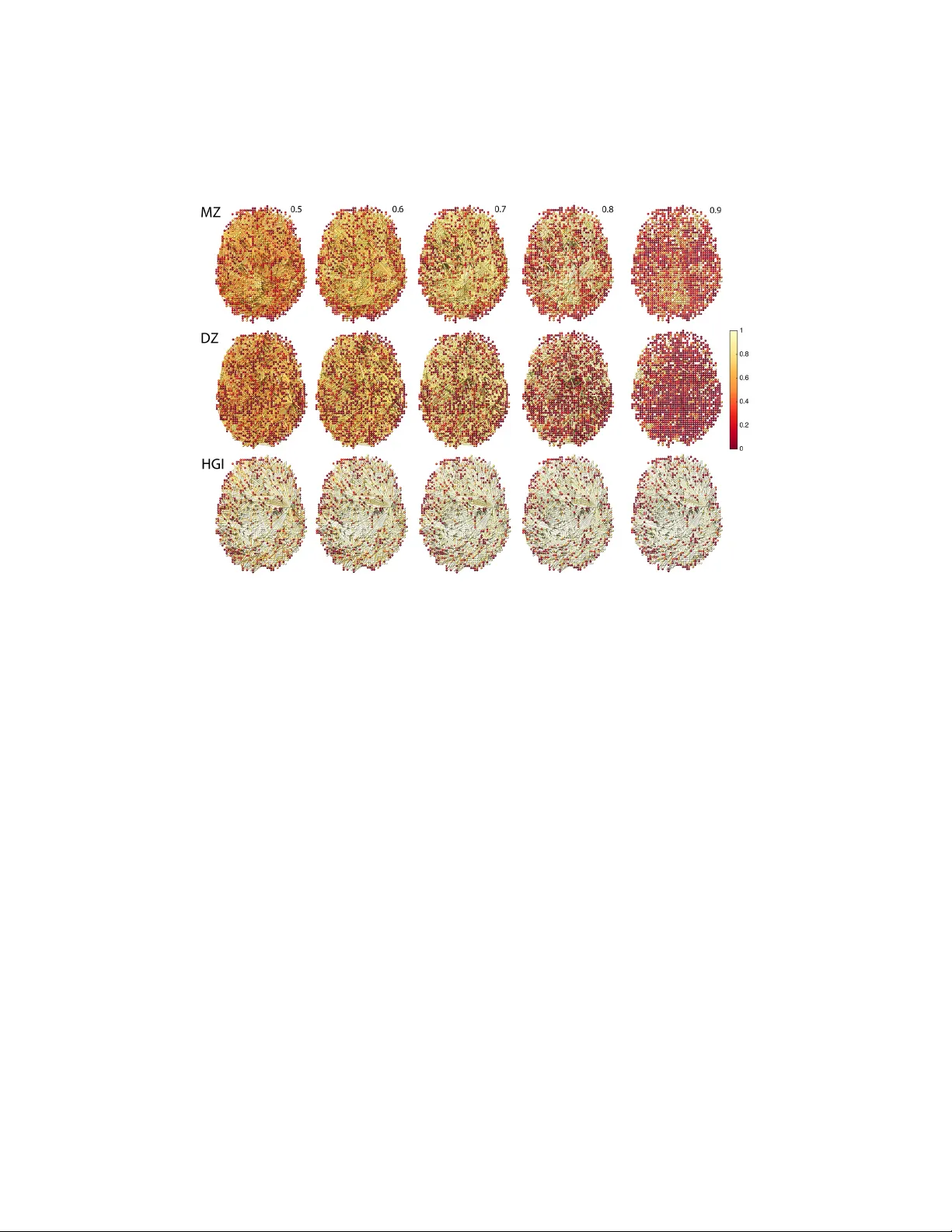
Mapping Heritabilit y of Large-Scale Brain Net w orks with a Billion Connections via P ersisten t Homology Mo o K. Ch ung 1 , Victoria Vilalta-Gil 2 , P aul J. Rathouz 1 , Benjamin B. Lahey 3 , Da vid H. Zald 2 1 Univ ersity of Wisconsin-Madison, 2 V anderbilt Univ ersity , 3 Univ ersity of Chicago email: mkchung@wisc.edu Septem b er 10, 2018 Abstract In man y human brain netw ork studies, w e do not hav e sufficient n umber ( n ) of images relative to the n umber ( p ) of v oxels due to the prohibitiv ely exp ensiv e cost of scanning enough sub jects. Thus, brain net work mo dels usually suffer the smal l-n lar ge-p pr oblem . Suc h a problem is often remedied b y sparse net w ork mo dels, which are usually solv ed numerically by optimizing L 1-p enalties. Unfortunately , due to the computational b ottleneck associated with optimizing L 1-p enalties, it is not practical to apply suc h metho ds to construct large-scale brain net works at the vo xel-level. In this pap er, w e propose a new scalable sparse net work mo del using cr oss-c orr elations that bypass the compu- tational b ottleneck. Our model can build sparse brain netw orks at the v oxel lev el with p > 25000. Instead of using a single sparse parameter that may not b e optimal in other studies and datasets, the computa- tional sp eed gain enables us to analyze the collection of net works at ev ery p ossible sparse parameter in a coheren t mathematical framework 1 via p ersistent homolo gy . The metho d is subsequently applied in deter- mining the extent of heritability on a functional brain net work at the v oxel-lev el for the first time using twin fMRI. 1 In tro duction L ar ge-sc ale br ain networks. In brain imaging, there hav e b een man y at- tempts to iden tify high-dimensional imaging features via m ultiv ariate ap- proac hes including net work features (Ch ung et al., 2013; Lerc h et al., 2006; He et al., 2007; W orsley et al., 2005a; Rao et al., 2008; Cao and W orsley, 1999; He et al., 2008). Sp ecifically , when the n umber of v oxels (often denoted as p ) are substan tially larger than the num b er of images (often denoted as n ), it produces an under-determined mo del with infinitely man y p ossible solutions. The small- n large- p problem is often remedied b y regularizing the under-determined system with additional sparse p enalties. P opular sparse mo dels include sparse correlations (Lee et al., 2011; Ch ung et al., 2013, 2015), LASSO (Bic kel and Levina, 2008; P eng et al., 2009; Huang et al., 2009; Chung et al., 2013), sparse canonical correlations (Av ants et al., 2010) and graphical-LASSO (Banerjee et al., 2006, 2008; F riedman et al., 2008; Huang et al., 2009, 2010; Mazumder and Hastie, 2012; Witten et al., 2011). Most of these s parse mo dels require optimizing L 1-norm p enalties, which has b een the ma jor computational b ottleneck for solving large-scale prob- lems in brain imaging. Th us, almost all sparse brain netw ork mo dels in brain imaging hav e b een restricted to a few hundreds no des or less. As far as we are aw are, 2527 MRI features used in a LASSO mo del for Alzheimer’s disease (Xin et al., 2015) is probably the largest n umber of features used in an y sparse mo del in the brain imaging literature. In this pap er, w e prop ose a new scalable large-scale sparse net work mo del ( p > 25000) that yields greater computational sp eed and efficiency by by- passing the computational b ottlenec k of optimizing L 1-p enalties. There are few previous studies at sp eeding up the computation for sparse mo dels. By 2 iden tifying blo c k diagonal structures in the estimated (inv erse) cov ariance matrix, it is p ossible to reduce the computational burden in the p enalized log-lik eliho o d method (Mazumder and Hastie, 2012; Witten et al., 2011). Ho wev er, the prop osed metho d substan tially differs from Mazumder and Hastie (2012) and Witten et al. (2011) in that w e do not need to assume that the data to follow Gaussianness. Subsequently , there is no need to spec- ify the lik eliho o d function. F urther, the cost functions we are optimizing are differen t. Sp ecifically , we prop ose a nov el sparse netw ork mo del based on cr oss-c orr elations . Although cross-correlations are often used in sciences in connection to times series and stochastic processes (W orsley et al., 2005a,b), the sparse version of cross-correlation has b een somewhat neglected. Persistent network homolo gy. An y sparse mo del G ( λ ) is usually param- eterized b y a tuning parameter λ that controls the sparsity of the repre- sen tation. Increasing the sparse parameter makes the solution more sparse. Sparse mo dels are inherently m ultiscale, where the scale of the mo dels is determined b y the sparse parameter. Ho wev er, many existing sparse net- w ork approac hes use a fixed parameter λ that may not b e optimal in other datasets or studies (Chung et al., 2013; Lee et al., 2012). Dep ending on the c hoice of the sparse parameter, the final classification and statistical results will b e totally different (Lee et al., 2012; Ch ung et al., 2013, 2015). Th us, there is a need to dev elop a multiscale netw ork analysis framew ork that pro vides a consistent statistical results and interpretation regardless of the c hoice of parameter. P ersisten t homology , a branch of algebraic top ology , offers one p ossible solution to the m ultiscale problem (Carlsson and Mem- oli, 2008; Edelsbrunner and Harer, 2008). Instead of looking at images and net works at a fixed scale, as usually done in traditional analysis approaches, p ersisten t homology observes the changes of top ological features ov er differ- en t scales and finds the most p ersistent top ological features that are robust under noise p erturbations. This robust p erformance under different scales 3 is needed for most netw ork mo dels that are parameter and scale dep endent. In this pap er, instead of building netw orks at one fixed sparse parameter that may not b e optimal, w e prop ose to build the collection of sparse mod- els ov er every possible sparse parameter using a gr aph filtr ation , a p ersistent homological construct (Chung et al., 2013; Lee et al., 2012). The graph filtration is a threshold-free framework for analyzing a family of graphs but requires hierarc hically building sp ecific nested subgraph structures. The pro- p osed metho d share some similarities to the existing multi-thresholding or m ulti-resolution netw ork mo dels that use many differen t arbitrary thresh- olds or scales (Ac hard et al., 2006; He et al., 2008; Kim et al., 2015; Lee et al., 2012; Sup ek ar et al., 2008). Ho wev er, such approaches ha ve not often applied to sparse mo dels ev en in an ad-ho c fashion b efore. Additionally , building sparse mo dels for multiple sparse parameters can causes an addi- tional computational b ottleneck to the already computationally demanding problem as w ell as introducing an additional problem of choosing optimal parameters. The prop osed p ersisten t homological approac h can address all these shortcomings within a unified mathematical framew ork. Heritability of br ain networks. Man y brain imaging studies hav e shown the widespread heritabilit y of neuroanatomical structures in magnetic res- onance imaging (MRI) (McKay et al., 2014) and diffusion tensor imaging (DTI) (Chiang et al., 2011). Ho wev er, these structural imaging studies use univ ariate imaging phenotypes such as cortical thic kness and fractional anisotrop y (F A) in determining heritabilit y at each vo xel or regions of in- terest. There are also few fMRI and EEG studies that use functional acti- v ations as p ossible imaging phenot yp es at eac h vo xel (Blokland et al., 2011; Glahn et al., 2010; Smit et al., 2008). Compared to many existing studies on univ ariate phenotypes, there are not many studies on the heritability of brain netw orks (Blokland et al., 2011). Measures of net work top ology and features ma y be w orth in vestigating as intermediate phenotypes or en- 4 dophenot yp es, that indicate the genetic risk for a neuropsychiatric disorder (Bullmore and Sp orns, 2009). Ho wev er, the brain net work analysis has not y et b een adapted for this purp ose. Determining the extent of heritability of brain net works with large n umber of no des is the first necessary prerequisite for iden tifying netw ork-based endophenotypes. This requires constructing the large-scale brain netw orks b y taking every vo xel in the brain as netw ork no des with at least a billion connections, whic h is a serious computational burden. Motiv ated by these neuroscientific and methodological needs, we pro- p ose to dev elop algorithms for building large-scale brain netw orks based on sp arse cr oss-c orr elations . The prop osed sparse netw ork mo del is used in constructing large-scale brain netw orks at the vo xel lev el in fMRI consisting of monozygotic (MZ) and dizygotic (DZ) twin pairs. The twin study design in brain imaging offers a v ery effective w ay of determining the heritability of the multiple features of the human brain. Heritabilit y (broad sense) can b e measured b y comparing the resemblance among monozygotic (MZ) t wins and dizygotic (DZ) twins using F alconer’s metho d (F alconer and Mack a y, 1995; T enesa and Haley, 2013) at the v oxel-lev el. As a w a y of quantify- ing the genetic contribution of phenot yp es, the heritability index (HI) has b een extensiv ely used in twin studies. Heritability index (HI) is the the amoun t of genetic v ariations in a phenotype. F or instance, 60% HI implies the phenotype is 60% heritable and 40% environmen tal. Except for few w ell kno wn neural circuits (Glahn et al., 2010; v an den Heuv el et al., 2013), the exten t to whic h heritabilit y influences functional brain netw orks at the v oxel-lev el is not w ell established. Although HI is a w ell formulated concept, it is unclear ho w to b est apply HI to netw orks. In this pap er, w e generalize the v oxel-wise univ ariate heritability index (HI) in to a netw ork-lev el multi- v ariate feature called heritability gr aph index (HGI), which is subsequen tly used in determining the genetic effects at the netw ork-lev el. The prop osed framew ork is used to determine the first-ever vo xel-level heritability map of 5 functional brain netw ork. 2 Metho ds 2.1 Sparse Cross-Correlations Let V = { v 1 , · · · , v p } b e a no de set where data is observed. W e expect the num b er of nodes p to b e significantly larger than the num b er of images n , i.e., p  n . In this study , we hav e p = 25972 vo xels in the brain that serv es as the no de set. Let x k ( v i ) and y k ( v i ) b e the k -th paired scalar measuremen ts at no de v i . Denote x ( v i ) = ( x 1 ( v i ) , · · · , x n ( v i )) 0 and y ( v i ) = ( y 1 ( v i ) , · · · , y n ( v i )) 0 b e the paired data v ectors o ver n differen t images at v oxel v i . Cen ter and scale x and y such that n X k =1 x k ( v i ) = n X k =1 y k ( v i ) = 0 , k x ( v i ) k 2 = x 0 ( v i ) x ( v i ) = k y ( v i ) k 2 = y 0 ( v i ) y ( v i ) = 1 for all v i . The reasons for cen tering and scaling will so on b e obvious. W e set up a linear mo del b etw een x ( v i ) and y ( v j ): y ( v j ) = b ij x ( v i ) + e , (1) where e is the zero-mean error vector whose comp onen ts are indep endent and identically distributed. Since the data are all centered, w e do not ha v e the intercept in linear regression ( 1 ). The least squares estimation (LSE) of b ij that minimizes the L2-norm p X i,j =1 k y ( v j ) − b ij x ( v i ) k 2 (2) is given by b b ij = x 0 ( v i ) y ( v j ) , (3) 6 whic h are the (sample) cr oss-c orr elations (W orsley et al., 2005a,b). The cross-correlation is inv ariant under the centering and scaling op erations. The sparse version of L2-norm ( 2 ) is given by F ( β ; x , y , λ ) = 1 2 p X i,j =1 k y ( v j ) − β ij x ( v i ) k 2 + λ p X i,j =1 | β ij | . (4) The sp arse cr oss-c orr elation is then obtained by minimizing ov er ev ery p os- sible β ij ∈ R : b β ( λ ) = arg min β F ( β ; x , y , λ ) . (5) The estimated sparse cross-correlations b β ( λ ) = ( b β ij ( λ )) shrink to ward zero as sparse parameter λ ≥ 0 increases. The direct optimization of ( 4 ) for large p is computationally demanding. How ever, there is no nee d to optimize ( 4 ) n umerically using the coordinate descen t learning or the active-set algorithm as often done in sparse optimization (P eng et al., 2009; F riedman et al., 2008). W e can show that the minimization of ( 4 ) is simply done algebraically . Prop osition 1. F or λ ≥ 0 , the minimizer of F ( β ; x , y , λ ) is given by b β ij ( λ ) =          x 0 ( v i ) y ( v j ) − λ if x 0 ( v i ) y ( v j ) > λ 0 if | x 0 ( v i ) y ( v j ) | ≤ λ x 0 ( v i ) y ( v j ) + λ if x 0 ( v i ) y ( v j ) < − λ . (6) See Appendix for pro of. Although it is not ob vious, Prop osition 1 is related to the orthogonal design in LASSO (Tibshirani, 1996) and the soft- shrink age in wa velets (Donoho et al., 1995). T o see this, let us transform linear equations ( 1 ) in to a index-free matrix equation:        y ( v 1 ) · · · y ( v 1 ) y ( v 2 ) · · · y ( v 2 ) . . . . . . . . . y ( v p ) · · · y ( v p )        =        b 11 x ( v 1 ) b 21 x ( v 2 ) · · · b p 1 x ( v p ) b 12 x ( v 1 ) b 22 x ( v 2 ) · · · b p 2 x ( v p ) . . . . . . . . . . . . b 1 p x ( v 1 ) b 2 p x ( v 2 ) · · · b pp x ( v p )        +        e · · · e e · · · e . . . . . . . . . e · · · e        . (7) 7 Equation ( 7 ) can b e vectorized as follo ws.                 y ( v 1 ) . . . y ( v p ) . . . y ( v 1 ) . . . y ( v p )                 =                 x ( v 1 ) · · · 0 . . . . . . . . . 0 · · · x ( v 1 ) · · · 0 . . . . . . . . . 0 · · · x ( v p ) · · · 0 . . . . . . . . . 0 · · · x ( v p )                                 b 11 . . . b p 1 . . . b 1 p . . . b pp                 +                 e . . . e . . . e . . . e                 . (8) ( 8 ) can b e written in a more compact form. Let X n × p = [ x ( v 1 ) x ( v 2 ) · · · x ( v p )] Y n × p = [ y ( v 1 ) y ( v 2 ) · · · y ( v p )] 1 a × b =     1 1 · · · 1 . . . . . . . . . . . . 1 1 · · · 1     a × b . Then ( 8 ) can b e written as 1 p × 1 ⊗ v ec ( Y ) = X np 2 × p 2 v ec ( b ) + 1 np 2 × 1 ⊗ e , (9) where ve c is the v ectorization op eration. The blo c k diagonal design matrix X consists of p diagonal blo cks I p ⊗ x ( v 1 ) , · · · , I p ⊗ x ( v p ), where I p is p × p iden tity matrix. Subseqeuntly , X 0 X is again a blo c k diagonal matrix, where the i -th blo ck is [ I p ⊗ x ( v i )] 0 [ I p ⊗ x ( v i )] = I p ⊗ [ x ( v i ) 0 x ( v i )] = I p . Th us, X is an orthogonal design. Ho w ever, our form ulation is not exactly the orthogonal design of LASSO as specified in Tibshirani (1996) since the noise comp onents in ( 9 ) are not indep enden t. F urther in standard LASSO, there are more columns than rows in X . In our case, there are n times more ro ws. 8 Figure 1: T op: The sparse cross-correlations are estimated by minimizing the L1 cost function ( 4 ) for 4 differen t sparse parameters λ (Prop osition 1 ). The edge weigh ts shrinked to zero are remov ed. Bottom: the equiv alen t bi- nary graph can b e obtained b y the simple soft-thresholding rule (Prop osition 2 ), i.e., simply thresholding the sample cross-correlations at λ . The num b er of clusters (denoted as #) and the size of the largest cluster (denoted as &) are display ed o ver different λ v alues. Prop osition 1 generalizes the sparse correlation case giv en in (Chung et al., 2013). Figure 1 -top displays an example of obtaining sparse cross- correlations from the initial sample cross-correlation matrix X 0 Y =     × 0.4 0.5 -0.7 × × 0.3 -0.1 × × × 0.9     using Prop osition 1 . F or simplicity , only the upp er triangle part of the sample cross-correlation is demonstrated. 9 2.2 Graph Filtrations F rom estimated sparse cross-correlations b β ( λ ), w e will first build the graph represen tation for subsequent brain netw ork quantification. Instead of try- ing to determine the optimal parameter λ and fix λ as often done in many sparse net w ork mo dels (Peng et al., 2009; Huang et al., 2009; Xin et al., 2015), w e will analyze the sparse net works ov er every p ossible λ . A single optimal parameter may not b e universally optimal across different datasets or ev en sufficient. This new approach enables us to build a m ultiscale net- w ork framew ork ov er sparse parameter λ . Definition 1. Supp ose weighte d gr aph G = ( V , W ) is forme d by the p air of no de set V = { v 1 , · · · , v p } and e dge weights W p × p = ( w ij ) . L et 0 and + λ b e binary op er ations on weighte d gr aphs such that G 0 = ( V , W 0 ) , W 0 = ( w 0 ij ) and G + λ = ( V , W + λ ) , W + λ = ( w + λ ij ) with w 0 ij =    1 if w ij 6 = 0; 0 otherwise and w + λ ij =    1 if w ij > λ ; 0 otherwise . The op erations 0 and + threshold edge weigh ts and make the w eighted graph binary . Definition 2. F or gr aphs G 1 = ( V , W ) , W = ( w ij ) and G 2 = ( V , Z ) , Z = ( z ij ) , G 2 is a subset of G 1 , i.e., G 1 ⊃ G 2 , if w ij ≥ z ij for al l i, j . The c ol le ction of neste d sub gr aphs G 1 ⊃ G 2 ⊃ · · · ⊃ G k is c al le d a gr aph filtr ation. k is the level of the filtr ation. Definition 2 extends the concept of the graph filtration heuristically given in Lee et al. (2012) and Ch ung et al. (2013), where only undirected graphs are considered, to more general directed graphs. Graph filtrations is a sp ecial case of Rips filtrations often studied in p ersisten t homology (Carlsson and 10 Memoli, 2008; Edelsbrunner and Harer, 2008; Singh et al., 2008; Ghrist, 2008). F rom Definitions 1 and 2 , for arbitrary weigh ted graph G = ( V , W ), w e ha v e G + λ 1 ⊃ G + λ 2 ⊃ G + λ 3 ⊃ · · · (10) for an y λ 1 ≤ λ 2 ≤ λ 3 · · · . Figure 1 -b ottom illustrates a graph filtration obtained with + op eration. Using these concepts, w e will build p ersisten t homology on sparse net- w ork G ( λ ) = ( V , b β ( λ )) with sparse cross-correlations b β ( λ ) obtained from ( 5 ). F or this, w e will first construct the collection of infinitely many binary graphs {G 0 ( λ ) : λ ∈ R + } . Prop osition 2. L et G 0 ( λ ) b e the binary gr aph obtaine d fr om sp arse network G ( λ ) = ( V , b β ( λ )) wher e b β ( λ ) ar e sp arse c orr elations. Consider another gr aph H = ( V , ρ ) , wher e the e dge weights ρ ij = | x ( v i ) 0 y ( v j ) | ar e the sample cr oss- c orr elations. Then, we have the fol lowing. (1) Soft-thr esholding rule: G 0 ( λ ) = H + λ for al l λ ≥ 0 . (2) The c ol le ction of binary gr aphs {G 0 ( λ ) : λ ∈ R + } forms a gr aph filtr ation. (3) Or der e dge weights ρ ij such that ρ (0) = 0 ≤ ρ (1) = min i,j ρ ij ≤ · · · ≤ ρ ( q ) = max i,j ρ ij . Then, for any λ ≥ 0 , G 0 ( λ ) = H + ρ ( i ) for some i . See App endix for pro of. Prop osition 2 -(1) enables us to construct large- scale sparse netw orks b y the simple soft thr esholding rule. This completely b ypasses numerical optimizations that hav e b een the main computational b ottlenec k in the field. Figure 1 illustrates the soft-thresholding rule in obtaining the equiv alent sparse binary graph without optimization. Prop osition 2 -(2) and 2 -(3) further sho w that w e can monotonically map the collection of constructed graphs {G 0 ( λ ) : λ ∈ R + } in to finite graph filtration H + ρ (0) ⊃ H + ρ (1) ⊃ · · · ⊃ H + ρ ( q ) . (11) 11 Figure 2: The result of graph filtrations on t win fMRI data. The num b er of disjoin t clusters (left) and the size of largest cluster (right) are plotted o ver the filtration v alues. A t a given filtration v alue, MZ-t wins hav e smaller n umber of clusters but larger cluster size. F or a graph with p no des, the maximum p ossible n umber of edges is ( p 2 − p ) / 2, which is obtained in a complete graph. ( p 2 − p ) / 2 + 1 is the upp er limit for the lev el of filtration in ( 11 ). 2.3 Statistical Inference on Graph Filtrations W e prop ose a new statistical inference pro cedure for p ersisten t homology . The metho d is applicable to many filtrations in p ersistent homology includ- ing Rips, Morse as w ell as graph filtrations. W e apply monotonic graph functions as multiscale features for statistical inference. Definition 3. L et # G b e the numb er of c onne cte d c omp onents (or disjoint clusters) of gr aph G and & G b e the size of the lar gest c omp onent (or cluster) of G . The graph functions # and & are monotonic o v er graph filtrations. F or filtration G 1 ⊃ G 2 ⊃ · · · , Note #( G 1 ) ≤ #( G 2 ) ≤ · · · and &( G 1 ) ≥ &( G 2 ) ≥ · · · . Figure 1 illustrates this monotonicity on the 4-no des sparse net work. 12 Prop osition 3. L et M b e the minimum sp anning tr e e (MST) of weighte d gr aph G = ( V , ρ ) with e dge wights ρ = ( ρ ij ) . Supp ose the e dge weights of M ar e sorte d as ρ (0) = −∞ ≤ ρ (1) ≤ · · · ≤ ρ ( p − 1) . Then for al l λ , # M + ρ ( i ) = # G + λ ≤ # M + ρ ( i +1) for some i . See App endix for pro of. W e do not sho w it here but an analogue state- men t can b e similarly obtained for &( G ). Prop osition 3 can b e used to monotonic al ly map infinitely many G + λ to only p n umber of sorted features # M +( −∞ ) ≤ # M + ρ (1) ≤ · · · ≤ # M + ρ ( p − 1) . (12) Similarly , we can monotonically map G + λ as & M +( −∞ ) ≥ & M + ρ (1) ≥ · · · ≥ & M + ρ ( p − 1) . (13) Figure 2 displa ys the plot of the n umber of clusters and the size of the largest cluster ov er filtration v alues for our t win fMRI data with p = 25972 no des. There are clear group discriminations. The statistical significance for of the discrimination can b e computed as follows. Let B i ( λ ) b e monotonic graph functions, such as # and &, ov er graph filtrations G + λ i . Then we are interested in testing the null hypothesis H 0 of the equiv alence of the tw o set of monotonic functions: H 0 : B 1 ( λ ) = B 2 ( λ ) for all λ. As a test statistic, we prop ose to use D p = sup λ | B 1 ( λ ) − B 2 ( λ ) | , whic h can b e view ed as the distance b et ween tw o graph filtrations. The test statistic D p is related to the t wo-sample Kolmogorov e-Smirnov (KS) test statistic (Chung et al., 2013; Gibb ons and Chakrab orti, 2011; B¨ ohm and Hornik, 2010). The test statistic takes care of the multiple comparisons o ver sparse parameters so there is no need to apply additional multiple comparisons correction pro cedure. The asymptotic probability distribution of D p can b e determined. 13 Prop osition 4. lim p →∞ P ( D p / p 2( p − 1) ≤ d ) = 1 − 2 P ∞ i =1 ( − 1) i − 1 e − 2 i 2 d 2 . See App endix for pro of. Note Prop osition 4 is nonparametric test and do es not assume an y statistical distribution other than that B 1 and B 2 are monotonic. F rom Prop osition 4 , p -v alue under H 0 is computed as p -v alue = 2 e − d 2 o − 2 e − 8 d 2 o + 2 e − 18 d 2 o · · · , where d o is the observed v alue of D p / p 2( p − 1) in the data. F or an y large observ ed v alue d 0 ≥ 2, the second term is in the order of 10 − 14 and insignif- ican t. Even for small observ ed d 0 , the expansion con verges quickly . 2.4 V alidation Study The prop osed metho d w as v alidated in t wo simulations with the kno wn ground truths. The simulations were p erformed 1000 times and the a verage results were rep orted. There are three groups and the sample size is n = 20 in each group and the num b er of no des are p = 100. In Group 1 and 2, data x k ( v i ) at no de v i w as simulated as standard normal, i.e., x k ( v i ) ∼ N (0 , 1). The paired data was— simulated as y k ( v i ) = x k ( v i ) + N (0 , 0 . 02 2 ) for all the no des. The simulated netw orks can b e found in Figure 3 . F ollowing the prop osed metho d, w e obtained the p -v alues of 0 . 712 ± 0 . 331 and 0 . 462 ± 0 . 413 for the num b er of clusters and the size of largest cluster. W e could not detect an y group differences as exp ected. Group 3 was generated identically but indep enden tly lik e Group 1 and 2 but additional dep endency was added. F or ten no des indexed b y j = 1 , 2 , · · · , 10, we simulated y k ( v j ) = x k ( v 1 ) + N (0 , 0 . 02 2 ) . This dep endency giv es high connection differences b etw een Groups 1 and 3. The simulated net work can b e found in Figure 3 . W e obtained the p -v alues of 0 . 025 ± 0 . 020 and 0 . 004 ± 0 . 010 for the num b er of clusters and the size of largest cluster demonstrating that we can detect the net work differences as exp ected. 14 Figure 3: Simulation studies. Three groups are sim ulated. Group 1 and Group 2 are generated indep endently but iden tically . The resulting B ( λ ) plots are similar. The dotted red line is the num b er of clusters and the solid blac k line is the size of the largest cluster. No statistically significan t differences can b e found betw een Groups 1 and 2. Group 3 is generated indep enden tly but identically as Group 1 but additional dep endency is added for the first 10 no des. The resulting B ( λ ) plots show statistically significant differences. This simulation is repeatedly done 1000 times. 3 Application 3.1 Twin fMRI Dataset The study consists of 11 monozygotic (MZ) and 9 same-sex dizygotic (DZ) t win pairs of 3T functional magnetic resonance images (fMRI) acquired in Intera-Ac hiav a Phillips MRI scanners with a state-of-the-art 32 channel SENSE head coil. Research was appro ved through the V anderbilt Univ er- sit y Institutional Review Board (IRB). Blo o d oxygenation-lev el dep endent (BOLD) functional images were acquired with a gradient echoplanar se- 15 quence, with 38 axial-oblique slices (3 mm thick, 0.3 mm gap), 80 × 80 in plane resolution, TR (repetition time) 2000 ms, TE (echo time) 25 ms, flip angle = 90. Sub jects completed monetary incen tive delay task (Kn utson et al., 2001) of 3 runs of 40 trials. A total 120 trials consisting of 40 $0, 40 $1 and 40 $5 rewards were pseudo randomly split in to 3 runs. The aim of the task is to rapidly resp ond to a target in order to earn rewards. T rials b egin with a cue indicating the amoun t of money that’s at stake for that sp ecific trial, then there is a delay p erio d b etw een the cue and the target in whic h participants prepare for the target to app ear. Then a white star (target) flashes rapidly on the screen. If the participants hit the resp onse button while the star is on the screen win the money . If they hit to o late, they do not win the money . After the resp onse, and a brief delay a feedback slide is sho wn indicating to the participan ts whether they hit the target on time or not and the amount of money they made for that sp ecific trial. The fMRI dimensions after preprocessing are 53 × 63 × 46 and the v oxel size is 3mm cub e. There are a total of p = 25972 vo xels in the brain tem- plate. Figure 4 shows the outline of the template. fMRI data wen t through spatial normalization to a template following the standard SPM pip eline (P enny et al., 2011). Images w ere processed with Gaussian k ernel smoothing with 8mm full-width-at-half-maximum (FWHM) spatially . Neuroscientifi- cally , we are interested in kno wing the extent of the genetic influenc e on the functional br ain networks of these participants while anticipating the high rew ard as measured by activity during the delay that o ccurs b et ween the rew ard cue and the target. After fitting a general linear mo del at each v o xel (F riston et al., 1995; Penn y et al., 2011), w e obtained contrast maps testing the significance of activity in the delay p erio d for $5 trials relative to the no rew ard control condition (Figure 4 ). The contrast maps w ere then used as the initial data v ectors x and y in our starting mo del ( 1 ). /Users/mo o c hung/Google Drive/t winstudy/pap ers/arxiv.v2-2016/ch ung.2016.06.29.p df 16 Figure 4: Representativ e MZ- and DZ-twin pairs of the contrast maps ob- tained from the first lev el analysis testing the significance of the dela y in hitting the resp onse button in $5 reward in con trast to $0 reward. Middle: The correlation of the con trast maps within each t win t yp es. Bottom: The heritabilit y index measures twice the difference b et ween the correlations. 3.2 In terc hangeablility of Data The sparse cross-correlations b β = ( b β ij ) are asymmetric and induce di- rected binary graphs. Supp ose there is no preference in data vectors x and y and they are in terchangeable. Our twin data is one of those inter- c hangeable cases since there is no preference of one t win o ver the other. Then we hav e another linear mo del, where x and y are in terchanged in ( 1 ): x ( v j ) = c ij y ( v i ) +  . The LSE of c ij is b c ij = y 0 ( v i ) x ( v j ). The symmetric version of (sample) cross-correlation ζ = ( ζ ij ) is then given b y 17 2 ζ ij = b b ij + b c ij = x 0 ( v i ) y ( v j ) + y 0 ( v i ) x ( v j ) . Similarly , the symmetric version of sparse cross-correlation η = ( η ij ) is obtained as 2 η = arg min β F ( β ; x , y ) + arg min γ F ( γ ; y , x ) . F or our study , each symmetrized cross-correlation ma- trix requires computing 1.3 billion entries and 5.2GB of computer memory (Figure 5 ). Since the cross-correlation matrices are very dense, it is diffi- cult to provide biological in terpretation and in terpretable data visualization. That is the main biological reason w e developed the prop osed sparse mo del to reduce the n umber of connections and come up with meaningful inter- pretation. All the statemen ts and metho ds presen ted here are applicable to symmeterized cross-correlations as well. T o see this, define the sum of graphs with identical no de set V as follows: Definition 4. F or gr aphs G 1 = ( V , W ) and G 2 = ( V , Z ) , G 1 + G 2 = ( V , W + Z ) . With Definition 4 , w e can sho w that the sum of an y tw o graph filtrations will b e again a graph filtration. Given tw o graph filtrations G 1 ⊂ G 2 ⊂ · · · ⊂ G k and H 1 ⊂ H 2 ⊂ · · · ⊂ H k , w e also ha ve G 1 + H 1 ⊂ G 2 + H 2 ⊂ · · · ⊂ G k + H k . Once we obtain the t wo sparse cross-correlations b β and b γ , construct w eighted graphs G 1 ( λ ) = ( V , b β ( λ )) and G 2 ( λ ) = ( V , b γ ( λ )). Then construct graph filtrations G 1 ( λ ) 0 and G 2 ( λ ) 0 . Using sample cross-correlations X 0 Y and Y 0 X , we can also define weigh ted graphs H 1 = ( V , X 0 Y ) and H 2 = ( V , Y 0 X ). Then construct binary graphs H + λ 1 and H + λ 2 . W e ha ve already sho wn that G 0 1 ( λ ) = H + λ 1 and G 0 2 ( λ ) = H + λ 2 . Th us, we ha ve G 0 1 ( λ ) + G 0 2 ( λ ) = H + λ 1 + H + λ 2 (14) and ( 14 ) forms a graph filtration o v er λ . Th us, Prop osition 2 and other metho ds can b e extended to the sum of filtrations G 0 1 ( λ ) + G 0 2 ( λ ) as well. 18 Figure 5: Cross-correlations for MZ- and DZ-twins for all 25972 v oxels in the brain template. There are more than 0.67 billion cross-correlations b e- t ween vo xels. Since the correlation matrices are to o dense to visualize and in terpret, it is necessary to reduce the n umber of connections. The diagonal en tries are P earson correlations. 3.3 Heritabilit y Graph Index The prop osed metho ds are applied in extending the vo xel-level univ ariate genetic feature called heritability index (HI) into a netw ork-lev el m ultiv ariate feature called heritability gr aph index (HGI). HGI is then used in determin- ing the genetic effects by constructing large-scale HGI by taking every vo xel as net w ork no des. HI determines the amount of v ariation (in terms of p er- cen tage) due to genetic influence in a population. HI is often estimated using F alconer’s formula (F alconer and Mack ay, 1995). MZ-twins share 100% of genes while DZ-twins share 50% genes. Th us, the additiv e genetic factor A , the common environmen tal factor C for eac h twin type are related as ρ MZ ( v i ) = A + C , (15) ρ DZ ( v i ) = A/ 2 + C., (16) where ρ MZ and ρ DZ are the pairwise correlation b etw een MZ- and and same- sex DZ-twins. Solving ( 15 ) and ( 16 ) at each vo xel v i , we obtain the additive 19 genetic factor or HI given by HI i = 2[ ρ MZ ( v i ) − ρ DZ ( v i )] . HI is a univ ariate feature measured at eac h vo xel and do es not quantify if the c hange in one v oxel is related to other vo xels. W e can extend the concept of HI to the netw ork lev el by defining the heritability graph index (HGI): HGI ij = 2[ % MZ ( v i , v j ) − % DZ ( v i , v j )] , where % MZ and % DZ are the symmetrized cross-correlations betw een v o xels v i and v j for MZ- and DZ-twin pairs. Note that % MZ ( v i , v i ) = ρ MZ ( v i ) and % DZ ( v i , v i ) = ρ DZ ( v i ) and the diagonal entries of HGI is HI, i.e., HGI ii = HI i . HGI measures genetic contribution in terms of p ercentage at the netw ork lev el while generalizing the concept of HI. In Figure 6 -top and -middle, the no des are correlations ρ MZ ( v i ) and ρ DZ ( v i ) while the edges are cross- correlations % MZ ( v i , v j ) and % DZ ( v i , v j ) resp ectively . In Figure 6 -b ottom, the no des are HI while edges are off-diagonal en tries of HGI. T o obtain the statistical significance of the HGI, we computed statistic D p and used Prop osition 4 . F or our data, the observed d o is 2.40 for the n umber of clusters and 23.12 for the size of largest cluster. p -v alues are less than 0.00002 and 0.00001 resp ectiv ely indicating very strong significance of HGI. W e further chec ked the v alidit y of the prop osed metho d b y randomly p erm uting twin pairs such that w e pair tw o images if they are not from the same t win. These pairs are split in to half and the sparse cross-correlations and HGI are computed follo wing the prop osed pip eline. It is expected that w e should not detect an y signal b eyond random chances. Figure 7 shows an example of sparse cross-correlation for one set of randomly paired images. As exp ected, ev en at sparse parameter λ = 0 . 5, there are not many significan t connections. A t sparse parameter λ = 0 . 7, there is no significan t connections at all. In comparison, w e are detecting extremely dense connections for b oth 20 Figure 6: T op and Middle: No de colors are correlations of MZ- and DZ- t wins. Edge colors are sparse cross-correlations at giv en sparsit y λ . Bottom: no de colors are heritability indices (HI) and edge colors are heritabilit y graph index (HGI). MZ-t wins show higher correlations at b oth vo xel and net work lev els compared to DZ-t wins. Some lo w HI no des sho w high HGI. Using only the vo xel-level HI feature will fail to detect suc h subtle genetic effects on the functional net work. MZ- and DZ-twins clearly demonstrating the high cross-correlations are due to the group lab eling and not due to random c hances. 4 Conclusion In this pap er, w e explored the computational issues of constructing large- scale brain netw orks within a unified mathematical framework integrating sparse net work mo del building, parameter estimation and statistical infer- 21 Figure 7: T op and Middle: No de colors are correlations of MZ- and DZ- t wins. Edge colors are sparse cross-correlations at giv en sparsit y λ . Bottom: no de colors are heritability indices (HI) and edge colors are heritabilit y graph index (HGI). MZ-t wins show higher correlations at b oth vo xel and net work lev els compared to DZ-t wins. Some lo w HI no des sho w high HGI. Using only the vo xel-level HI feature will fail to detect suc h subtle genetic effects on the functional net work. ence on graph filtrations. Although the method is applied in t win fMRI data to address the problem of determining the genetic con tribution to functional brain net w orks, it can be applied to other more general problems of correlat- ing paired data suc h as m ultimo dal fMRI to PET. W e believe the theoretical framew ork presented here provides a motiv ation for future works on v arious fields dealing with paired functional data and net works. 22 App endix Pr o of to Pr op osition 1. W rite F ( β ; x , y , λ ) as F ( β ; x , y , λ ) = 1 2 p X i,j =1 f ( β ij ) , where f ( β ij ) = k y ( v j ) − β ij x ( v i ) k 2 +2 λ | β ij | . Since f ( β ij ) is nonnegative and conv ex, F ( β ; x , y , λ ) is minimum if each comp onen t f ( β ij ) ac hieves its minimum. So we only need to minimize each comp onen t f ( β ij ) separately . Using the constrain t k x ( v i ) k = 1, f ( γ j k ) is simplified as 1 − 2 β ij x ( v i ) 0 y ( v j ) + β 2 ij + 2 λ | β ij | = ( β ij − x ( v i ) 0 y ( v j )) 2 + 2 λ | β ij | + 1 − [ x ( v i ) 0 y ( v j )] 2 . F or λ = 0, the minim um of f ( β ij ) is achiev ed when β ij = x ( v i ) 0 x ( v j ), whic h is the usual least squares estimation (LSE). F or λ > 0, Since f ( β ij ) is quadratic, the minim um is ac hieved when ∂ f ∂ β ij = 2 β ij − 2 x 0 ( v i ) y ( v j ) ± 2 λ = 0 . (17) The sign of λ dep ends on the sign of β ij . By rearranging terms, w e obtain the desired result.  Pr o of to Pr op osition 2. (1) The adjacency matrix A = ( a ij ) of G 0 ( λ ) is giv en by a ij = 1 if b β ij ( λ ) 6 = 0 and a ij = 0 otherwise . F rom Prop osition 1 , b β ij ( λ ) 6 = 0 if | x ( v i ) 0 y ( v j ) | > λ and b β ij ( λ ) = 0 if | x ( v i ) 0 y ( v j ) | ≤ λ . Th us, adjacency matrix A is equiv alent to another adjacency matrix B = ( b ij ) giv en b y b ij ( λ ) =    1 if | ρ ij | > λ ; 0 otherwise . (18) 23 On the other hand, the adjacency matrix of binary graph H + λ is exactly giv en b y B . Th us G 0 ( λ ) = H + λ . (2) F or all 0 ≤ λ 1 ≤ λ 2 ≤ · · · , b ij ( λ 1 ) ≥ b ij ( λ 2 ) ≥ · · · for all i, j . Hence, H + λ 1 ⊃ H + λ 2 ⊃ · · · and equiv alently , G 0 ( λ 1 ) ⊃ G 0 ( λ 2 ) ⊃ · · · . So the collection of G 0 ( λ ) forms a graph filtration. (3) If 0 = ρ (0) ≤ λ < ρ (1) , G 0 ( λ ) = H + ρ (0) . If ρ ( i ) ≤ λ < ρ ( i +1) , G 0 ( λ ) = H + ρ ( i ) for 1 ≤ i ≤ q − 1. F or ρ ( q ) ≤ λ , G 0 ( λ ) = H + ρ ( q ) , the no de set. Thus G 0 ( λ ) = H + ρ ( i ) for any λ ≥ 0 for some i .  Pr o of to Pr op osition 3. F or a tree with p no des, there are p − 1 edges with edge weigh ts sorted as ρ (1) = min i,j ρ ij ≤ ρ (2) ≤ · · · ≤ ρ ( p − 2) ≤ ρ ( p − 1) = max i,j ρ ij . No edge weigh ts are ab ov e ρ ( p − 1) , thus when thresholded at ρ ( p − 1) , all the edges are remo v ed and end up with node set V . Thus, # M + ρ ( p − 1) = p . Since all edges are ab ov e 0, # M + ρ (0) = 1. F or any graph G with p no des and an y λ , 1 ≤ # G + λ ≤ p . Th us, the ranges of # G + λ and # M + ρ ( i ) matc h. There exists some ρ ( i ) satisfying # G + λ = # M + ρ ( i ) for some i . Note # M + ρ ( i +1) ≥ # M + ρ ( i ) + 1. Therefore, # G + λ ≤ # M + ρ ( i +1) .  Pr o of to Pr op osition 4. Let M i b e the MST of graph G i . F rom the pro of of Prop osition 3 , the range of function # M + λ i exactly matches the range of function B i ( λ ). Th us, we ha ve sup λ | B 1 ( λ ) − B 2 ( λ ) | = sup i   # M + ρ ( i ) 1 − | # M + ρ ( i ) 2   . Therefore, the problem is equiv alent to testing the equiv alence of t wo set of paired monotonic v ectors ( M + ρ (0) 1 , · · · , M + ρ ( p − 1) 1 ) and ( M + ρ (0) 2 , · · · , M + ρ ( p − 1) 2 ). 24 Com bine these tw o vectors and arrange them in increasing order. Represen t # M + ρ ( i ) 1 and # M + ρ ( i ) as x and y resp ectively . Then the combined v ectors can be represented as, for example, xxy xy x · · · . T reat the sequence as w alks on a Cartesian grid. x indicates one step to the righ t and y indicates one step up. Then from grid (0 , 0) to ( p − 1 , p − 1), there are total  2 p − 2 p − 1  p os- sible n umber of paths. Then following closely the argument given in pages 192-194 in Gibb ons and Chakrab orti (2011) and B¨ ohm and Hornik (2010) w e ha v e P  D p p − 1 ≥ d  = 1 − A p − 1 ,p − 1  2 p − 2 p − 1  , (19) where A p − 1 ,p − 1 = A p − 1 ,p − 2 + A p − 2 ,p − 1 with b oundary conditions A (0 , p − 1) = A ( p − 1 , 0) = 1. Then asymptotically ( 19 ) can b e written as (Smirno v, 1939) lim p →∞  D p p − 1 ≥ d  = 1 − 2 ∞ X i =1 ( − 1) i − 1 e − 2 i 2 d 2 .  Ac kno wledgmen ts This work w as supp orted by NIH Researc h Grant 5 R01 MH098098 04. W e thank Y uan W ang at the Univ ersity of Wisconsin-Madison, Zhiw ei Ma at Tsingh ua Universit y , Matthew Arnold of Universit y of Bristol for v aluable discussions ab out the KS-lik e test procedure prop osed in this study . References S. Achard, R. Salv ador, B. Whitcher, J. Suckling, and E.D. Bullmore. A resilient, lo w-frequency , small-w orld human brain functional net work with highly con- nected asso ciation cortical hubs. The Journal of Neur oscienc e , 26:63–72, 2006. B.B. Av ants, P .A. Co ok, L. Ungar, J.C. Gee, and M. Grossman. Demen tia in- duces correlated reductions in white matter integrit y and cortical thickness: a m ultiv ariate neuroimaging study with sparse canonical correlation analysis. Neu- r oImage , 50:1004–1016, 2010. 25 O. Banerjee, L.E. Ghaoui, A. d’Aspremont, and G. Natsoulis. Conv ex optimization tec hniques for fitting sparse Gaussian graphical mo dels. In Pr o c e e dings of the 23r d International Confer enc e on Machine L e arning , page 96, 2006. O. Banerjee, L. El Ghaoui, and A. d’Aspremon t. Mo del selection through sparse maxim um likelihoo d estimation for multiv ariate Gaussian or binary data. The Journal of Machine L e arning R ese ar ch , 9:485–516, 2008. P .J. Bick el and E. Levina. Regularized estimation of large cov ariance matrices. The Annals of Statistics , 36:199–227, 2008. G.A.M. Blokland, K.L. McMahon, P .M. Thompson, N.G. Martin, G.I. de Zubicaray , and M.J. W right. Heritabilit y of working memory brain activ ation. The Journal of Neur oscienc e , 31:10882–10890, 2011. W alter B¨ ohm and Kurt Hornik. A Kolmogoro v-Smirnov test for r samples. Institute for Statistics and Mathematics , Research Rep ort Series:Rep ort 105, 2010. E. Bullmore and O. Sporns. Complex brain netw orks: graph theoretical analysis of structural and functional systems. Natur e R eview Neur oscienc e , 10:186–98, 2009. J. Cao and K.J. W orsley . The geometry of correlation fields with an application to functional connectivity of the brain. A nnals of Applie d Pr ob ability , 9:1021–1057, 1999. G. Carlsson and F. Memoli. Persisten t clustering and a theorem of J. Klein b erg. arXiv pr eprint arXiv:0808.2241 , 2008. M.-C. Chiang, K.L. McMahon, G.I. de Zubicaray , N.G. Martin, I. Hickie, A.W. T oga, M.J. W right, and P .M. Thompson. Genetics of white matter developmen t: a dti study of 705 t wins and their siblings aged 12 to 29. Neur oimage , 54:2308– 2317, 2011. M.K. Chung, J.L. Hanson, H. Lee, Nagesh Adluru, Andrew L. Alexander, R.J. Da vidson, and S.D. Pollak. P ersistent homological sparse netw ork approach to detecting white matter abnormality in maltreated children: MRI and DTI m ultimo dal study . MICCAI, L e ctur e Notes in Computer Scienc e (LNCS) , 8149: 300–307, 2013. 26 M.K. Chung, J.L. Hanson, Y e J., Davidson R.J., and Pollak S.D. Persisten t homol- ogy in sparse regression and its application to brain morphometry . IEEE T r ans- actions on Me dic al Imaging, ArXiv e-prints 1409.0177 , 34:1928–1939, 2015. D.L. Donoho, I.M. Johnstone, G. Kerkyac harian, and D. Picard. W av elet shrink age: asymptopia? Journal of the R oyal Statistic al So ciety. Series B (Metho dolo gic al) , 57:301–369, 1995. H. Edelsbrunner and J. Harer. P ersisten t homology - a surv ey . Contemp or ary Mathematics , 453:257–282, 2008. D. F alconer and T Mac k ay . Intr o duction to Quantitative Genetics, 4th e d. Longman, 1995. J. F riedman, T. Hastie, and R. Tibshirani. Sparse inv erse cov ariance estimation with the graphical lasso. Biostatistics , 9:432, 2008. K.J. F riston, A.P . Holmes, K.J. W orsley , J.-P . P oline, C.D. F rith, and R.S.J. F rack- o wiak. Statistical parametric maps in functional imaging: A general linear ap- proac h. Human Br ain Mapping , 2:189–210, 1995. R. Ghrist. Barco des: The p ersisten t top ology of data. Bul letin of the Americ an Mathematic al So ciety , 45:61–75, 2008. J. D. Gibb ons and S. Chakrab orti. Nonp ar ametric Statistic al Infer enc e . Chapman & Hall/CRC Press, 2011. D.C. Glahn, A.M. Winkler, P . Ko c huno v, L. Almasy , R. Duggirala, M.A. Carless, J.C. Curran, R.L. Olv era, A.R. Laird, S.M. Smith, C.F. Beckmann, P .T. F ox, and J. Blangero. Genetic control ov er the resting brain. Pr o c e e dings of the National A c ademy of Scienc es , 107:1223–1228, 2010. Y. He, Z.J. Chen, and A.C. Ev ans. Small-world anatomical netw orks in the human brain rev ealed b y cortical thic kness from MRI. Cer ebr al Cortex , 17:2407–2419, 2007. Y. He, Z. Chen, and A. Ev ans. Structural insigh ts in to aberrant top ological patterns of large-scale cortical net works in Alzheimer’s disease. Journal of Neur oscienc e , 28:4756, 2008. 27 S. Huang, J. Li, L. Sun, J. Liu, T. W u, K. Chen, A. Fleisher, E. Reiman, and J. Y e. Learning brain connectivit y of Alzheimer’s disease from neuroimaging data. In A dvanc es in Neur al Information Pr o c essing Systems , pages 808–816, 2009. S. Huang, J. Li, L. Sun, J. Y e, A. Fleisher, T. W u, K. Chen, and E. Reiman. Learning brain connectivit y of Alzheimer’s disease by sparse inv erse cov ariance estimation. Neur oImage , 50:935–949, 2010. W.H. Kim, N. Adluru, M.K. Ch ung, O.C. Okonkw o, S.C. Johnson, B. Bendlin, and V. Singh. Multi-resolution statistical analysis of brain connectivit y graphs in preclinical Alzheimers disease. Neur oImage , 118:103–117, 2015. B. Kn utson, C.M. Adams, G.W. F ong, and D. Hommer. Anticipation of increas- ing monetary reward selectively recruits nucleus accumbens. Journal of Neur o- scienc e , 21:R C159, 2001. H. Lee, D.S.. Lee, H. Kang, B.-N. Kim, and M.K. Chung. Sparse brain netw ork reco very under compressed sensing. IEEE T r ansactions on Me dic al Imaging , 30: 1154–1165, 2011. H. Lee, H. Kang, M.K. Ch ung, B.-N. Kim, and D.S Lee. P ersistent brain netw ork homology from the p ersp ectiv e of dendrogram. IEEE T r ansactions on Me dic al Imaging , 31:2267–2277, 2012. J.P . Lerch, K. W orsley , W.P . Shaw, D.K. Greenstein, R.K. Lenro ot, J. Giedd, and A.C. Ev ans. Mapping anatomical correlations across cerebral cortex (MA CACC) using cortical thickness from MRI. Neur oImage , 31:993–1003, 2006. R. Mazumder and T. Hastie. Exact cov ariance thresholding into connected com- p onen ts for large-scale graphical LASSO. The Journal of Machine L e arning R ese ar ch , 13:781–794, 2012. D.R. McKa y , E.E.M. Knowles, A.A.M. Winkler, E. Sprooten, P . Ko ch uno v, R.L. Olv era, J.E. Curran, J.W. Kent Jr., M.A. Carless, H.H.H. G¨ oring, T.D. Dyer, R. Duggirala, L. Almasy , P .T. F ox, J. Blangero, and D.C. Glahn. Influence of age, sex and genetic factors on the human brain. Br ain imaging and b ehavior , 8: 143–152, 2014. 28 J. Peng, P . W ang, N. Zhou, and J. Zh u. Partial correlation estimation b y join t sparse regression models. Journal of the Americ an Statistic al Asso ciation , 104: 735–746, 2009. W.D. P enny , K.J. F riston, J.T. Ash burner, S.J. Kiebel, and T.E. Nic hols. Statistic al p ar ametric mapping: the analysis of functional br ain images: the analysis of functional br ain images . Academic press, 2011. A. Rao, P . Aljabar, and D. Rueck ert. Hierarchical statistical shap e analysis and prediction of sub-cortical brain structures. Me dic al Image Analysis , 12:55–68, 2008. G. Singh, F. Memoli, T. Ishkhanov, G. Sapiro, G. Carlsson, and D.L. Ringach. T op ological analysis of p opulation activity in visual cortex. Journal of Vision , 8:1–18, 2008. N.V. Smirnov. Estimate of deviation b et ween empirical distribution functions in t wo indep endent samples. Bul letin of Mosc ow University , 2:3–16, 1939. D.J.A. Smit, C.J. Stam, D. P osthuma, D.I. Bo omsma, and E.J.C. De Geus. Her- itabilit y of small-world netw orks in the brain: a graph theoretical analysis of resting-state EEG functional connectivity . Human br ain mapping , 29:1368–1378, 2008. K. Sup ek ar, V. Menon, D. Rubin, M. Musen, and M.D. Greicius. Netw ork analysis of intrinsic functional brain connectivit y in Alzheimer’s disease. PL oS Compu- tational Biolo gy , 4(6):e1000100, 2008. A. T enesa and C.S. Haley . The heritability of human disease: estimation, uses and abuses. Natur e R eviews Genetics , 14:139–149, 2013. R. Tibshirani. Regression shrink age and selection via the LASSO. Journal of the R oyal Statistic al So ciety. Series B (Metho dolo gic al) , 58:267–288, 1996. M.P . v an den Heuvel, I.L.C. v an So elen, C.J. Stam, R.S. Kahn, D.I. Bo omsma, and H.E. H. Pol. Genetic control of functional brain net work efficiency in children. Eur op e an Neur opsychopharmac olo gy , 23:19–23, 2013. 29 Daniela M Witten, Jerome H F riedman, and Noah Simon. New insigh ts and faster computations for the graphical lasso. Journal of Computational and Gr aphic al Statistics , 20:892–900, 2011. K.J. W orsley , A. Charil, J. Lerch, and A.C. Ev ans. Connectivit y of anatomical and functional MRI data. In Pr o c e e dings of IEEE International Joint Confer enc e on Neur al Networks (IJCNN) , volume 3, pages 1534–1541, 2005a. K.J. W orsley , J.I. Chen, J. Lerch, and A.C. Ev ans. Comparing functional connectiv- it y via thresholding correlations and singular v alue decomp osition. Philosophic al T r ansactions of the R oyal So ciety B: Biolo gic al Scienc es , 360:913, 2005b. B. Xin, L. Hu, Y. W ang, and W. Gao. Stable feature selection from brain sMRI. In Pr o c e e dings of the Twenty-Nineth AAAI Confer enc e on Artificial Intel ligenc e , 2015. 30