NN-grams: Unifying neural network and n-gram language models for Speech Recognition

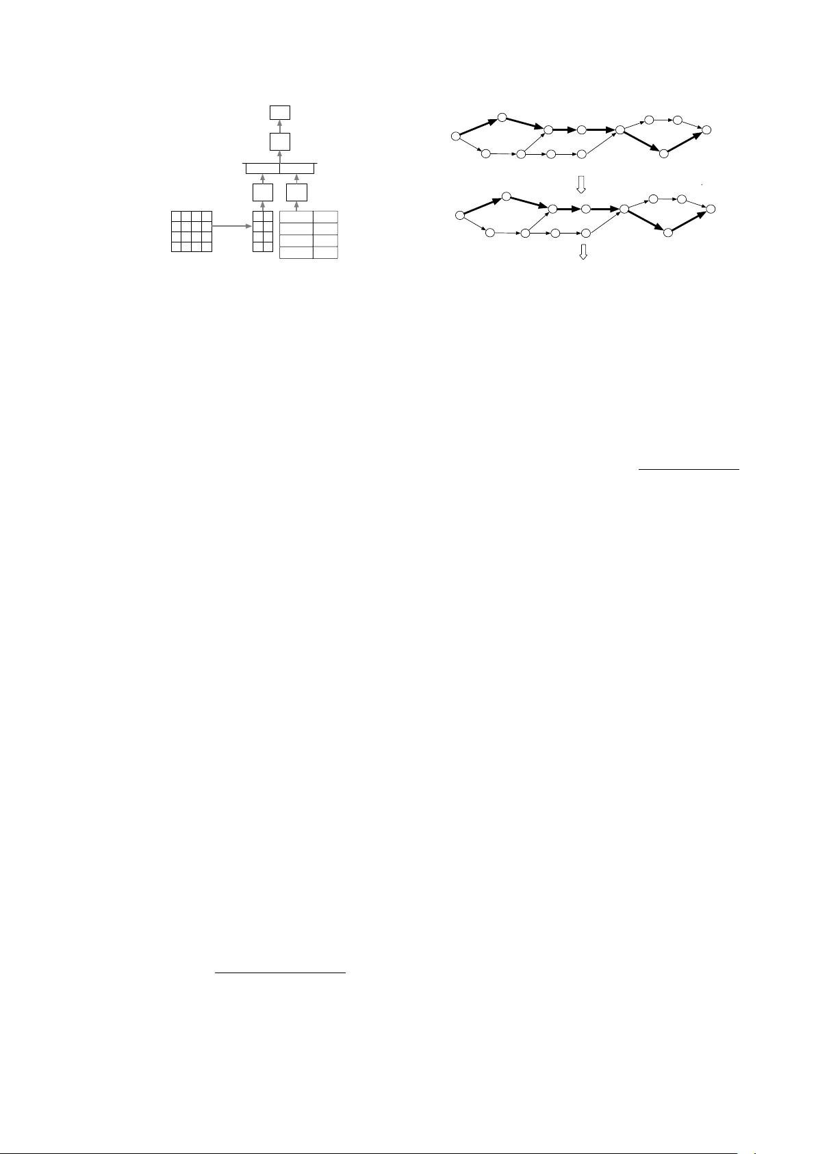
NN-grams: Unifying neural network and n-gram language models f or speech r ecognition Babak Damavandi, Shankar K umar , Noam Shazeer , Antoine Bruguier Google Inc., 1600 Amphitheatre Parkw ay , Mountain V ie w , CA 94043, USA { babakd,shankarkumar,noam,tonybruguier } @google.com Abstract W e present NN-grams, a nov el, hybrid language model inte- grating n-grams and neural networks (NN) for speech recog- nition. The model takes as input both word histories as well as n-gram counts. Thus, it combines the memorization capac- ity and scalability of an n-gram model with the generalization ability of neural networks. W e report experiments where the model is trained on 26B words. NN-grams are efficient at run- time since they do not include an output soft-max layer . The model is trained using noise contrastive estimation (NCE), an approach that transforms the estimation problem of neural net- works into one of binary classification between data samples and noise samples. W e present results with noise samples de- riv ed from either an n-gram distribution or from speech recog- nition lattices. NN-grams outperforms an n-gram model on an Italian speech recognition dictation task. Index T erms : speech recognition, language models, neural net- works 1. Introduction A language model (LM) is a crucial component of natural lan- guage processing technologies such as speech recognition [1] and machine translation [2]. It helps discriminate between well- formed and ill-formed sentences in a language. T raditionally , n-gram LMs hav e formed the basis for most language modeling approaches. It has only been in the past few years that alterna- tiv e approaches such as maximum-entrop y models [3] and neu- ral network models including feed-forward networks [4, 5, 6], recurrent neural netw orks (RNNs) [7] and v ariants such as long short term memory (LSTM) networks [8] have started outper - forming n-gram models [9]. Neural network LMs hav e advantages ov er n-gram mod- els. First, they provide better smoothing for rare and unknown words o wing to their distributed word representations [9]. Neu- ral network Models such as LSTMs hav e the ability to remem- ber long-distance context, an attrib ute that has eluded se veral language models in the past. Ev en with these potential advan- tages, LSTMs and other neural network models have not been used extensiv ely for language modeling in speech recognition because the y are more resource intensi ve at both training and run time when compared to n-gram models. This continues to be the case despite recent efforts at speeding up training and test times using techniques such as pipelined training and vari- ance regularization [10]. LSTMs do not scale well to the large quantities of text training data typically used for estimating n- gram LMs. This is a substantial disadv antage during training because a lar ger LSTM which attains a better performance than a smaller LSTM is also slower to conv erge. At run time, an LSTM is e xpensiv e in terms of both memory and speed rela- tiv e to an n-gram model. Specifically , the output soft-max layer is computationally expensi ve at both training and run time if the vocabulary size is in the order of millions of words, a com- mon characteristic of current speech recognition systems (e.g. [11]). Therefore, most neural network language modeling ap- proaches for speech recognition hav e employed smaller vocab- ularies consisting of at most several thousands of words [5, 7]. Speech recognizers for voice search and dictation typically op- erate on short utterances on which n-gram models perform fairly well. This has further limited the usefulness of LSTM LMs for these tasks. In this paper , we in vestig ate a flav or of neural network LMs that combines the strengths of a neural network in generalizing to novel contexts with the scalability and memorization ability of an n-gram model. Our main proposal is to train a neural net- work that is able to learn a mapping function given both the previous history of a giv en word as well as the n-gram counts, which are sufficient statistics for estimating an n-gram model. By providing n-gram counts as inputs, we expect this model to learn simultaneously a function of the counts as well as the word history and estimate the probability of the current word giv en the history . Specifically , this model is a feed-forward neural network that takes as input the current word, K previous words, and counts for the N n-grams ending at the current w ord, where N < K . W e call this model neural network-ngrams ( NN-grams ), to emphasize that it makes direct use of n-gram count statistics. While there have been earlier efforts at incor- porating hashes of n-gram features as inputs to an RNN [7], we are not aware of a neural network model that directly takes n-gram counts as inputs. T o reduce computation, we do not include an output soft- max layer in NN-grams. While the NN-grams’ score can be interpreted as a log probability of the current word gi ven the history , the absence of a soft-max layer means that these proba- bilities do not necessarily sum to one over the entire vocab ulary . 2. NN-grams An LM is a probability distrib ution ov er the current word giv en the preceding words: P ( w i | w i − 1 , w i − 2 , . . . , w 1 ) . An n-gram LM makes the assumption that the current word depends only on the previous N − 1 words: i.e. P ( w i | w i − 1 , . . . , w 1 ) = P ( w i | w i − 1 , . . . , w i − ( N − 1) ) . The architecture of the NN-grams model is giv en in Fig- ure 1. The model takes as input the current word, K preceding words and counts for the N n-grams ending at the current word and estimates the log likelihood of the current word given the history: n-gram counts Embedding ReLu A ReLu B Counts Embeddings ReLu C NCE Concat log P(alarm | please set an) please an alarm Input 1-hot vector set 0 1 0 0 0 1 0 1 0 0 0 0 0 0 0 1 - 0.1 0.9 -0.3 0.3 0.8 0.7 - 0.4 0.1 C(an) C(alarm) C(please) C(set) C(an alarm) C(set an) C(please set) 0 Figure 1: Arc hitectur e of the NN-grams model. The pr evious wor ds ar e “please” “set” “an” and the current word is alarm . N = 2 , K = 3 and the embedding dimension is 2. f nng ( w i , . . . , w 1 ) = log P ( w i | w i − 1 , . . . , w i − K , c ) where c is a vector of n-gram counts of length ( K + 1) N such that c 1 = Count ( w i ) , c 2 = Count ( w i , w i − 1 ) ,..., C N = Count ( w i , w i − 1 , . . . , w i − ( N − 1) ) are counts of n-grams ending at the current word, c N +1 through c 2 N are counts of n-grams ending at the pre vious w ord,..., and c K N +1 through c ( K +1) N are counts of n-grams ending at w ord w i − K (See the count ma- trix in Figure 1 for an example), and the log probability is esti- mated by the neural network. Each of the words w i , . . . , w i − K is presented as a 1-hot v ector to the netw ork. The number of previous words, K, can be larger than N, the order of the n-gram counts. This enables the model to take into account longer con- text. Like other neural network LMs [4], the NN-grams model maps words into a high dimensional space and learns an em- bedding for each word in this space while simultaneously also learning the network parameters. The word embeddings and the n-gram counts are passed through separate layers with rectified linear unit (ReLu) activ ations [12] and then concatenated. The result is passed through a third ReLu layer and provided as an input to NCE. The output of the NCE layer approximates the log probability of the current word giv en the history and the n-gram counts. Unlike other neural network language model- ing approaches [4, 5, 13], there is no explicit soft-max over the vocab ulary . 2.1. Model Estimation W e train the neural network using noise contrastiv e estimation (NCE), a method for training unnormalized probabilistic mod- els [14, 13, 15]. NCE transforms the estimation problem of the netw ork into a classification problem where the goal is to differentiate between samples from the training data ( D = 1 ) and those from a pre-specified noise distribution ( D = 0 ). For brevity , we abbreviate the current word, w i as w and its history w i − 1 . . . , w i − K , c as h . Our goal is to fit the neural network to the training data distribution P data ( w | h ) . Suppose we have f noise samples for each training data sample, the posterior probability that the sample ( h, w ) arises from the training data is giv en by [15]: P ( D = 1 | w , h ) = P data ( w | h ) P data ( w | h ) + P noise ( w | h ) f . W e estimate this probability by replacing the data distribution Hello W ell o how how now are are you you all to day well today Hello#1 W ell#1 o#1 how#2 how#2 now#2 are#3 are#3 you#4 you#4 well#5 to#6 day#6 all#5 today#6 Hello how are you all today W ell o now well to day T ruth Noise Figure 2: Extracting speech noise samples via lattice pinching. All hypotheses in a lattice (top panel) are aligned with respect to the 1-best hypothesis (shown in bold). F or each lattice edge, the alignment r elative to the 1-best hypothesis is determined (mid- dle panel). The list of noise samples is then extr acted for each position (bottom panel). log P data ( w | h ) with that of the neural network NN ( w, h ) : logit ( D = 1 | w , h ) = log  P ( D = 1 | w , h ) 1 − P ( D = 1 | w , h )  = log P data ( w | h ) − log ( f ) − log P noise ( w | h ) ≈ NN ( w, h ) − log ( f ) − log P noise ( w | h ) . 2.2. Noise Distributions NCE training works best when the noise distribution is close to the data distribution. In this case, the training data samples are hard to distinguish from noise samples and the model is forced to learn about the structure of the data [14]. W e experiment with two types of noise distributions. In the first type, we sample the noise word from the n-gram distribution over the words given the history . W e will refer to this as te xt noise . In the second type, we sample the noise word from the word le vel confusions generated from a speech recognition system. W e will refer to this as speech noise . Unlike text noise, speech noise consists of words which are acoustically confusable with the words in the training data. Ideally , these noise samples would be words which are tran- scribed incorrectly by the speech recognition system when com- pared with a human transcription. Howe ver , the quantity of hu- man transcriptions is limited. Therefore, we run the recognizer on utterances where human transcriptions are not av ailable and additionally , a 1-best recognition hypothesis with high confi- dence exists. The noise words are the alternativ es to the 1-best recognition h ypothesis. W e align the 1 -best hypothesis to the paths in the recognition word lattice using lattice pinching [16] (Figure 2) and obtain a set of noise samples for each word in the 1-best hypothesis. W ithin each such set, the noise proba- bility of a giv en word is its posterior probability . W e exclude those words in the 1-best hypothesis which a) do not hav e con- fusions in the lattice e.g. ar e and you in Figure 2, and b) align to word sequences with more than more word e.g. Hello aligns with well o in Figure 2. 2.3. Count Rescaling One of the inputs to NN-grams is a vector of n -gram counts. Since this count can hav e a large dynamic range from 0 to sev eral millions, we rescale the count to improv e the con ver - gence of neural network training using gradient descent [17]. If C is the original count, the rescaled count is obtained as C 0 = 0 . 1 log ( C ) if C > 0 and − 1 if C = 0 . 3. Experiments W e evaluated the NN-gram language model (LM) on Italian voice-search and dictation speech recognition tasks. Since the NN-gram model does not yield probability estimates that are guaranteed to be normalized, we do not report perplexities. Our test sets consisted of a voice-search (VS) set with 12,877 ut- terances (27.4 hours, 47,867 words) and a dictation (DTN) set with 12,625 utterances (19.2 hours, 82,121 words). All utter - ances were anonymized. The acoustic models were trained us- ing con volutional, LSTM, fully connected deep neural netw orks as described in [18]. All LMs were trained on anonymized and aggregated search queries and dictated texts. A 5-gram LM with Katz backoff was trained using a total of 26B words, and con- sisted of a total of 102M n-grams. The initial word lattice was generated using this 5-gram LM and a recognition vocabulary consisting of 3.9M words. The NN-grams model w as trained on the same corpus as the 5-gram LM. Since the NN-grams model takes 6-gram counts as input, we additionally trained a 6-gram LM with Katz backoff to provide a fair baseline. Prior work [19, 20] has sho wn that when using pruning, n-gram models with Katz backoff outper- form those with Kneser-Ney smoothing [21]. Hence, we used Katz back off as the smoothing technique for all our n-gram lan- guage models. W e limited the vocab ulary size to 2M words for both models. Even though the NN-grams model has fewer parameters than the 6-gram LM (T able 1), it requires the avail- ability of n-gram counts at run time. LM parameter type # of parameters 6gram n-grams 9.6B NNgram NN parameters 517M T able 1: Model Parameters of NN-grams and 6-gram LMs. The word lattices generated in the initial recognition pass were rescored using either the 6-gram LM or the NN-grams model. In the case of the NN-grams LM, there is no exact al- gorithm for rescoring the lattice. W e note that there hav e been approximate algorithms to rescore l attices using long-span neu- ral network language models [22, 23]. Ho wev er , we did not employ these lattice rescoring methods and instead, extracted and reranked the 150-best word hypotheses from the lattice. 1 The score (log probability) of the either the 6-gram LM or the NN-grams model was interpolated with the log probability of the 5-gram LM using a fixed weight of 0.5. The 5-gram LM gav e a W ord Error Rate (WER) of 17.9% on VS and 11.8% on DTN. W e set the parameters K and N of the NN-grams model to 9 and 6 respectiv ely . The model was trained until conv ergence with an AdaGrad optimizer [24] using a learning rate that was set to 0.01. W e used a batch size of 200 in training. The di- mensionality of the word embedding layer was 256. The ReLu layer that processed the embeddings (ReLu-A) had 1024 units while the Relu layer that processed the n-gram counts (ReLu-B) 1 If there were fewer than 150 hypotheses for an utterance, we ex- tracted the maximum number of av ailable hypotheses. had 256 units. Finally , the ReLu layer that processed the con- catenation of embeddings and counts (ReLu-C) had 1024 units. For NCE, we generated one noise sample for each word in the training data using text noise. 3.1. Comparison with n-gram LMs W e first compared the performance of NN-grams with the 6- gram LM. The results are shown in T able 2. When compared with the 6-gram LM, the NN-grams LM sho wed a better perfor- mance on the DTN task and an equivalent performance on the VS task. While additional gains might be potentially obtained by first rescoring the lattice with a 6-gram model followed by interpolation with NN-grams, such a system would be too slow to deploy in a speech recognition system with stringent latency requirements. Hence, we did not pursue such an interpolation. VS DTN 6-gram 14.9 8.8 NN-grams 14.8 8.2 T able 2: WER Comparison of NN-gr ams with 6-gr am LM on voice-sear ch and dictation. 3.2. NN-grams components NN-grams consist of two components: word embeddings and the n-gram counts. T o determine which of these two compo- nents had a bigger impact on the ov erall performance of the NN-grams model, we trained the model with either one of these inputs (Figure 1). For both VS and DTN, n-gram counts were more important than word embeddings (T able 3). W e expect this result considering that using n-gram counts typically im- prov es the performance for short sentences, which is the case for both VS and DTN (A verage number of words/sentence on VS and DTN is 3.7 and 6.5 respectively). For DTN, word embed- dings contrib uted to an additional improvement in WER, that can be attributed to the longer sentence length in DTN. NN-grams components VS DTN W ord-embedding,n-gram counts 14.8 8.2 W ord Embedding 15.3 8.8 n-gram Counts 14.9 8.5 T able 3: Impact of NN-grams components on WER. 3.3. T ype and Quantity of Noise Samples W e next examined whether the type and number of noise sam- ples influenced the performance of the NN-grams model (T a- ble 5). Since the speech noise samples can be obtained only from lattices, we restricted our training set in this e xperiment to only those utterances for which we were able to run the speech recognizer and generate word lattices. The training set con- sisted of 1.2B words from a subset of utterances derived from both voice search and dictation sources on which the 1-best recognition hypothesis had a high confidence. As a result, the WERs for these systems are worse than the system trained on 26B words (T able 2). The speech and the te xt noise samples were generated using the procedure described in Sec 2.2. The training data was annotated with n-gram counts deri ved from the 26B word corpus used in the earlier experiments. 1 Reference Poi ha detto per le sagome dei marmi del bagno e che quando lui tornav a dav a le misure per fare fare i marmi 1 n-gram poi ha detto per le sagome dei bei marmi del bagno ` e che quando lui torna da quale misura per fare fare i marmi 1 NN-grams poi ha detto per le sagome dei bei marmi del bagno ` e che quando lui tornav a dav a le misure per fare fare i marmi 2 Reference ` E molto pi ` u forte rispetto alle altre classi tipo Audi, Mercedes 2 n-gram ` e molto pi forte rispetto a Mercedes 2 NN-grams ` e molto pi forte rispetto ad altre classi tv Audi Mercedes 3 Reference Am mo mi puoi sposare C’abbiamo la casa c’abbiamo la chiesa e c’ ` e la sposa 3 n-gram am ` o mi puoi sposare se abbiamo la casa che abbiamo la Chiesa Ecce la sposa 3 NN-grams am ` o mi puoi sposare c’abbiamo la casa c’abbiamo la Chiesa e c’ ` e la sposa T able 4: Examples of recognition hypotheses where the NN-grams LM outperforms the n-gram LM. # of noise samples T ext Noise Speech Noise VS DTN VS DTN 1 19.2 11.6 21.7 14.5 5 19.4 12.3 20.9 14.1 10 20.1 12.6 20.4 13.9 100 17.3 10.6 17.5 12.3 T able 5: Impact of the type and number of noise samples on WER. For each type of noise, we report WER using 1, 5, 10 and 100 noise samples. For both types of noise, the best perfor- mance was seen at 100 samples per word. The text noise out- performed the speech noise on DTN but obtained an equi valent performance on VS. It is possible that text noise, that relies on an n-gram distribution, is more suited to the dictation task where long range context is useful. In contrast, the speech noise sam- ples which are acoustically confusable alternatives do not al- ways have long distance dependencies. Based on these results, we could e xpect additional gains using 100 noise samples in the original set up with 26B words (T able 2). 3.4. Embeddings In the NN-grams model, each word is mapped to a real valued vector . These w ord embeddings are key to the generalization capabilities of a neural network LM. W e present e xamples of the top-5 nearest neighbors for two Italian words, Roma and telefono computed using the word embedding estimated in the NN-grams model (T able 6). The nearest neighbors for Roma are all cities in Italy while those for telefono consist of terms related to communication and business. In general, these neigh- bors in the embedding space are related to the source word, thus emphasizing the semantic nature of the space. Roma telefono W ord ED W ord ED Bologna 1.08 cellulare 1.33 Milano 1.09 tel 1.34 Firenze 1.15 contatti 1.41 T orino 1.16 indirizzo 1.47 Napoli 1.17 fax 1.53 T able 6: T op-5 nearest neighbors for two Italian source words: Roma and telefono computed using the NN-grams word embed- dings. The Euclidean distance (ED) of each neighbor from the source word is also sho wn. 3.5. Examples W e present example recognition hypotheses where the NN- grams LM substantially outperformed the 6-gram LM (T able 4). In example 1, while the n-gram model prefers the common construction torna da (come back fr om) , NN-grams is either recognizing a complex construction or prefers the tense agree- ment between tornava and dava . In example 2, the n-gram LM prefers dropping clauses while NN-grams does not. In example 3, the NN-grams model is possibly recognizing the repeating pattern in the sentence C’abbiamo la casa c’abbiamo la chiesa e c’ ` e la sposa (we have a house, we have a churc h, we have a bride) while the n-gram model looks independently at each of the 3 phrases, se abbiamo , che abbiamo and Ecce , and mis- recognizes all of them. This last example may be a scenario where the long 10-word windo w of NN-grams giv es it a distinct advantage o ver the n-gram LM. 4. Discussion In this paper , we presented NN-grams, a nov el neural network language modeling framew ork that builds upon the memoriza- tion capabilities and scalability of n -gram LMs while still al- lowing us to benefit from the generalization capabilities of neu- ral networks. Our model obtains a 7% relativ e reduction in word error rate on an Italian dictation task. W e showed that the strength of the NN-grams model comes primarily from the n- gram counts but both n-gram counts and word embeddings are important for long-form content such as dictation. W e trained the model using NCE training with either text or speech noise distributions. While text noise is better for the dictation task, both noise types perform similarly for voice-search. The biggest disadvantage of the speech noise approach is that it requires decoding of utterances. Future work will in vestigate strategies which can directly generate acoustically confusable noise sam- ples from only text using strategies that have been in vestigated in the context of discriminativ e language modeling [25, 26]. These strate gies generate noise samples at either the phonetic or sub-phonetic (e.g. Gaussian) lev els. In conclusion, the NN- grams model is a promising neural network LM that is scalable to large training texts. By avoiding the output softmax layer , it has a substantially l ower ov erhead at training and run time com- pared to current neural network approaches such as LSTMs. W e expect that this model will spur newer hybrid architectures which will increase the adoption of neural network approaches to language modeling. 5. Acknowledgements W e would like to thank Kaisuke Nakajima, Xuedong Zhang, Francoise Beaufays, Chris Alberti and Rafal Jozefo wicz for pro- viding crucial support at various stages of this project. 6. References [1] F . Jelinek, Statistical Methods for Speech Recognition . Cam- bridge, MA, USA: The MIT Press, 1997. [2] P . F . Bro wn, J. Cocke, S. A. Della Pietra, V . J. . Della Pietra, F . Je- linek, J. D. Laf ferty , R. L. Mercer, and P . S. Roossin, “ A statistical approach to machine translation, ” vol. 16, no. 2, pp. 79–85, 1990. [3] S. F . Chen, “Shrinking exponential language models, ” in Pr oceed- ings of Human Language T echnologies: The 2009 Annual Confer - ence of the North American Chapter of the Association for Com- putational Linguistics . Association for Computational Linguis- tics, 2009, pp. 468–476. [4] Y . Bengio, R. Ducharme, P . V incent, and C. Jauvin, “ A neural probabilistic language model. 3: 1137–1155, ” J ournal of Mac hine Learning Resear ch , vol. 3, pp. 1137 – 1155, 2003. [5] H. Schwenk, “Continuous space language models, ” Comput. Speech Lang. , v ol. 21, no. 3, pp. 492–518, Jul. 2007. [6] E. Arisoy , T . N. Sainath, B. Kingsbury , and B. Ramabhadran, “Deep neural network language models, ” in Proceedings of the NAA CL-HL T 2012 W orkshop: W ill W e Ever Really Replace the N-gram Model? On the Future of Language Modeling for HLT , ser . WLM ’12. Stroudsbur g, P A, USA: Association for Compu- tational Linguistics, 2012, pp. 20–28. [7] T . Mik olov , A. Deoras, D. Povey , L. Burget, J. Cernock ` y, and S. Khudanpur, “Strategies for training large scale neural network language models, ” in ASRU , 2011, pp. 196–201. [8] S. Hochreiter and J. Schmidhuber , “Long short-term memory , ” Neural computation , v ol. 9, no. 8, pp. 1735–1780, 1997. [9] R. Jozefowicz, O. V inyals, M. Schuster, N. Shazeer , and Y . W u, “Exploring the limits of language modeling, ” arXiv pr eprint arXiv:1602:02410 , 2016. [10] X. Chen, X. Liu, M. Gales, and P . W oodland, “Improving the training and ev aluation efficiency of recurrent neural network language models, ” in Acoustics, Speech and Signal Processing (ICASSP), 2015 IEEE International Confer ence on . IEEE, 2015, pp. 5401–5405. [11] A. Senior , H. Sak, F . d. C. Quitry , T . N. Sainath, and K. Rao, “ Acoustic modelling with CD-CTC-SMBR LSTM RNNs, ” in ASR U . IEEE, 2015. [12] V . Nair and G. E. Hinton, “Rectified linear units improve restricted boltzmann machines, ” in Pr oceedings of the 27th International Confer ence on Machine Learning (ICML-10) , 2010, pp. 807–814. [13] A. Mnih and Y . W . T eh, “ A fast and simple algorithm for training neural probabilistic language models, ” arXiv preprint arXiv:1206.6426 , 2012. [14] M. Gutmann and A. Hyv ¨ arinen, “Noise-contrastiv e estimation: A new estimation principle for unnormalized statistical models, ” in International Conference on Artificial Intelligence and Statistics , 2010, pp. 297–304. [15] A. Mnih and K. Kavukcuoglu, “Learning word embeddings effi- ciently with noise-contrastive estimation, ” in Advances in Neural Information Pr ocessing Systems , 2013, pp. 2265–2273. [16] V . Goel, S. Kumar, and W . Byrne, “Segmental minimum bayes- risk decoding for automatic speech recognition, ” IEEE Tr ansac- tions on Speech and Audio Pr ocessing , v ol. 12, no. 3, pp. 234– 249, 2004. [17] Y . LeCun, L. Bottou, G. Orr , and K. Muller , “Ef ficient backprop, ” in Neural Networks: T ricks of the trade , G. Orr and M. K., Eds. Springer , 1998. [18] T . N. Sainath, O. V inyals, A. Senior, and H. Sak, “Con volutional, long short-term memory , fully connected deep neural networks, ” in 2015 IEEE International Confer ence on Acoustics, Speec h and Signal Pr ocessing (ICASSP) . IEEE, 2015, pp. 4580–4584. [19] C. Chelba, T . Brants, W . Nev eitt, and P . Xu, “Study on interaction between entropy pruning and kneser-ney smoothing. ” in INTER- SPEECH , 2010, pp. 2422–2425. [20] B. Roark, C. Allauzen, and M. Riley , “Smoothed marginal distri- bution constraints for language modeling. ” in ACL (1) , 2013, pp. 43–52. [21] R. Kneser and H. Ne y , “Improved backing-off for m-gram lan- guage modeling, ” in Acoustics, Speec h, and Signal Pr ocessing, 1995. ICASSP-95., 1995 International Conference on , vol. 1. IEEE, 1995, pp. 181–184. [22] M. Sundermeyer , Z. T ¨ uske, R. Schl ¨ uter , and H. Ney , “Lattice decoding and rescoring with long-span neural network language models. ” in INTERSPEECH , 2014, pp. 661–665. [23] X. Liu, Y . W ang, X. Chen, M. J. Gales, and P . C. W oodland, “Ef- ficient lattice rescoring using recurrent neural network language models, ” in Acoustics, Speech and Signal Processing (ICASSP), 2014 IEEE International Confer ence on . IEEE, 2014, pp. 4908– 4912. [24] J. Duchi, E. Hazan, and Y . Singer , “ Adaptive subgradient methods for online learning and stochastic optimization, ” The Journal of Machine Learning Resear ch , v ol. 12, pp. 2121–2159, 2011. [25] G. Kurata, N. Itoh, M. Nishimura, A. Sethy , and B. Ramabhadran, “Lev eraging word confusion networks for named entity model- ing and detection from conversational telephone speech, ” Speech Commun. , vol. 54, no. 3, pp. 491–502, Mar . 2012. [26] P . Jyothi and E. Fosler-Lussier , “Discriminative language mod- eling using simulated asr errors. ” in INTERSPEECH , 2010, pp. 1049–1052.