Explaining Predictions of Non-Linear Classifiers in NLP

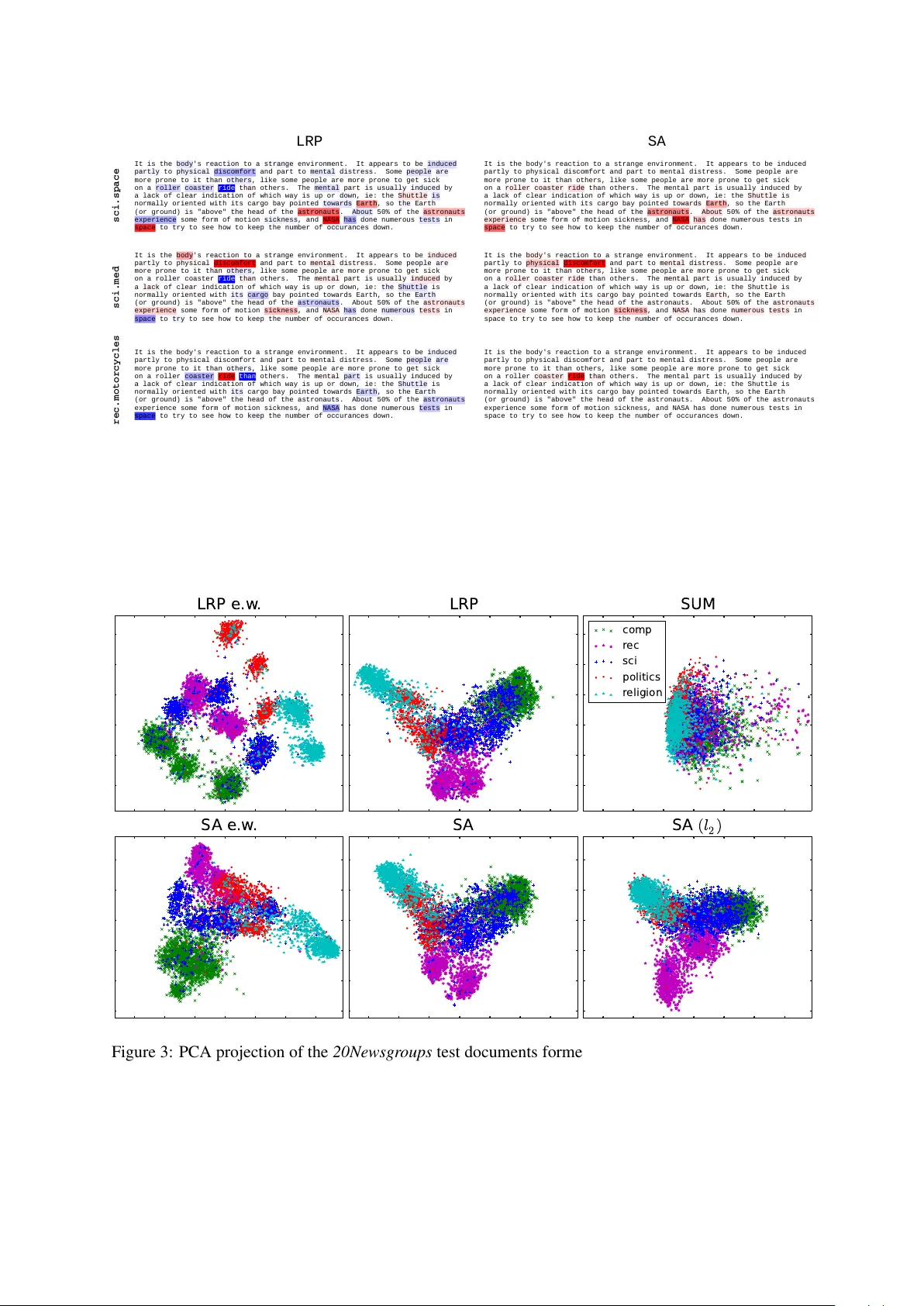
Explaining Pr edictions of Non-Linear Classifiers in NLP Leila Arras 1 , Franziska Horn 2 , Gr ´ egoire Monta von 2 , Klaus-Robert M ¨ uller 2 , 3 , and W ojciech Samek 1 1 Machine Learning Group, Fraunhofer Heinrich Hertz Institute, Berlin, Germany 2 Machine Learning Group, T echnische Univ ersit ¨ at Berlin, Berlin, Germany 3 Department of Brain and Cogniti ve Engineering, K orea Univ ersity , Seoul, K orea { leila.arras, wojciech.samek } @hhi.fraunhofer.de klaus-robert.mueller@tu-berlin.de Abstract Layer-wise rele vance propagation (LRP) is a recently proposed technique for e x- plaining predictions of complex non-linear classifiers in terms of input v ariables. In this paper , we apply LRP for the first time to natural language processing (NLP). More precisely , we use it to explain the predictions of a conv olutional neural net- work (CNN) trained on a topic categoriza- tion task. Our analysis highlights which words are rele vant for a specific prediction of the CNN. W e compare our technique to standard sensitivity analysis, both qual- itati vely and quantitati vely , using a “word deleting” perturbation experiment, a PCA analysis, and various visualizations. All experiments v alidate the suitability of LRP for explaining the CNN predictions, which is also in line with results reported in re- cent image classification studies. 1 1 Introduction Follo wing seminal work by Bengio et al. (2003) and Collobert et al. (2011), the use of deep learn- ing models for natural language processing (NLP) applications recei ved an increasing attention in re- cent years. In parallel, initiated by the computer vision domain, there is also a trend to ward under- standing deep learning models through visualiza- tion techniques (Erhan et al., 2010; Landecker et al., 2013; Zeiler and Fergus, 2014; Simonyan et al., 2014; Bach et al., 2015; Lapuschkin et al., 2016a) or through decision tree extraction (Krish- nan et al., 1999). Most work dedicated to under- standing neural netw ork classifiers for NLP tasks 1 Paper will appear in the Proceedings of the 1st W ork- shop on Representation Learning for NLP at Association for Computational Linguistics Conference (A CL 2016). (Denil et al., 2014; Li et al., 2015) use gradient- based approaches. Recently , a technique called layer-wise relev ance propagation (LRP) (Bach et al., 2015) has been shown to produce more mean- ingful explanations in the context of image classi- fications (Samek et al., 2015). In this paper , we ap- ply the same LRP technique to a NLP task, where a neural network maps a sequence of word2vec vectors representing a text document to its cat- egory , and ev aluate whether similar benefits in terms of explanation quality are observ ed. In the present work we contribute by (1) ap- plying the LRP method to the NLP domain, (2) proposing a technique for quantitati ve e valuation of explanation methods for NLP classifiers, and (3) qualitati vely and quantitati vely comparing two dif ferent explanation methods, namely LRP and a gradient-based approach, on a topic categorization task using the 20Newsgr oups dataset. 2 Explaining Predictions of Classifiers W e consider the problem of explaining a predic- tion f ( x ) associated to an input x by assigning to each input variable x d a score R d determining how rele vant the input v ariable is for explaining the prediction. The scores can be pooled into groups of input variables (e.g. all wor d2vec dimensions of a word, or all components of a RGB pixel), such that they can be visualized as heatmaps of high- lighted texts, or as images. 2.1 Layer -Wise Rele vance Propagation Layer-wise relev ance propagation (Bach et al., 2015) is a newly introduced technique for obtain- ing these e xplanations. It can be applied to v arious machine learning classifiers such as deep conv olu- tional neural networks. The LRP technique pro- duces a decomposition of the function value f ( x ) on its input variables, that satisfies the conserv a- tion property: f ( x ) = P d R d . (1) The decomposition is obtained by performing a backward pass on the network, where for each neuron, the relev ance associated with it is redis- tributed to its predecessors. Considering neurons mapping a set of n inputs ( x i ) i ∈ [1 ,n ] to the neuron acti vation x j through the sequence of functions: z ij = x i w ij + b j n z j = P i z ij x j = g ( z j ) where for con venience, the neuron bias b j has been distributed equally to each input neuron, and where g ( · ) is a monotonously increasing activ ation function. Denoting by R i and R j the rele vance associated with x i and x j , the rele vance is redis- tributed from one layer to the other by defining messages R i ← j indicating ho w much rele v ance must be propagated from neuron x j to its input neuron x i in the lo wer layer . These messages are defined as: R i ← j = z ij + s ( z j ) n P i z ij + s ( z j ) R j where s ( z j ) =  · (1 z j ≥ 0 − 1 z j < 0 ) is a stabilizing term that handles near-zero denominators, with  set to 0 . 01 . The intuition behind this local rele- v ance redistrib ution formula is that each input x i should be assigned relev ance proportionally to its contribution in the forward pass, in a way that the rele vance is preserved ( P i R i ← j = R j ). Each neuron in the lo wer layer receives rele- v ance from all upper-le vel neurons to which it con- tributes R i = P j R i ← j . This pooling ensures layer -wise conserv ation: P i R i = P j R j . Finally , in a max-pooling layer , all relev ance at the output of the layer is redistrib uted to the pooled neuron with max- imum activ ation (i.e. winner-take-all). An im- plementation of LRP can be found in (La- puschkin et al., 2016b) and do wnloaded from www.heatmapping.org 2 . 2 Currently the av ailable code is targeted on image data. 2.2 Sensitivity Analysis An alternativ e procedure called sensitivity analy- sis (SA) produces explanations by scoring input v ariables based on how they affect the decision output locally (Dimopoulos et al., 1995; Gevre y et al., 2003). The sensiti vity of an input variable is gi ven by its squared partial deriv ativ e: R d =  ∂ f ∂ x d  2 . Here, we note that unlike LRP , sensiti vity analysis does not preserve the function v alue f ( x ) , but the squared l 2 -norm of the function gradient: k∇ x f ( x ) k 2 2 = P d R d . (2) This quantity is howe ver not directly related to the amount of e vidence for the category to de- tect. Similar gradient-based analyses (Denil et al., 2014; Li et al., 2015) hav e been recently applied in the NLP domain, and were also used by Simon yan et al. (2014) in the conte xt of image classification. While recent work uses different rele v ance defini- tions for a group of input variables (e.g. gradient magnitude in Denil et al. (2014) or max -norm of absolute value of simple deri vati ves in Simonyan et al. (2014)), in the present work (unless other- wise stated) we employ the squared l 2 -norm of gradients allowing for decomposition of Eq. 2 as a sum ov er relev ances of input variables. 3 Experiments For the following experiments we use the 20ne ws- bydate version of the 20Ne wsgroups 3 dataset con- sisting of 11314/7532 train/test documents e venly distributed among twenty fine-grained cate gories. 3.1 CNN Model As a document classifier we employ a word-based CNN similar to Kim (2014) consisting of the fol- lo wing sequence of layers: Conv − → ReLU − → 1-Max-Pool − → FC By 1-Max-Pool we denote a max-pooling layer where the pooling regions span the whole text length, as introduced in (Collobert et al., 2011). Conv , ReLU and FC denote the con- volutional layer , rectified linear units activ ation and fully-connected linear layer . For b uilding 3 http://qwone.com/%7Ejason/20Newsgroups/ the CNN numerical input we concatenate horizon- tally 300-dimensional pre-trained word2vec 4 vec- tors (Mikolo v et al., 2013), in the same order the corresponding words appear in the pre-processed document, and further keep this input representa- tion fixed during training. The con volutional oper- ation we apply in the first neural network layer is one-dimensional and along the text sequence di- rection (i.e. along the horizontal direction). The recepti ve field of the con volutional layer neurons spans the entire word embedding space in verti- cal direction, and cov ers two consecuti ve w ords in horizontal direction. The con volutional layer filter bank contains 800 filters. 3.2 Experimental Setup As pre-processing we remov e the document head- ers, tokenize the text with NL TK 5 , filter out punc- tuation and numbers 6 , and finally truncate each document to the first 400 tokens. W e train the CNN by stochastic mini-batch gradient de- scent with momentum (with l 2 -norm penalty and dropout). Our trained classifier achie ves a classifi- cation accuracy of 80.19% 7 . Due to our input representation, applying LRP or SA to our neural classifier yields one relev ance v alue per word-embedding dimension. From these single input variable relev ances to obtain word- le vel relev ances, we sum up the relev ances over the word embedding space in case of LRP , and (unless otherwise stated) tak e the squared l 2 -norm of the corresponding word gradient in case of SA. More precisely , gi ven an input document d consisting of a sequence ( w 1 , w 2 , ..., w N ) of N words, each word being represented by a D - dimensional word embedding, we compute the rel- e vance R ( w t ) of the t th word in the input docu- ment, through the summation: R ( w t ) = D X i =1 R i,t (3) 4 GoogleNews-vectors-negative300, https://code.google.com/p/word2vec/ 5 W e employ NL TK’ s version 3.1 recommended tok- enizers sent tokenize and word tokenize , module nltk.tokenize . 6 W e retain only tokens composed of the following char- acters: alphabetic-character, apostrophe, h yphen and dot, and containing at least one alphabetic-character . 7 T o the best of our kno wledge, the best published 20Newsgr oups accurac y is 83.0% (Pasko v et al., 2013). How- ev er we notice that for simplification we use a fixed-length document representation, and our main focus is on explain- ing classifier decisions, not on improving the classification state-of-the-art. where R i,t denotes the rele vance of the input v ari- able corresponding to the i th dimension of the t th word embedding, obtained by LRP or SA as spec- ified in Sections 2.1 & 2.2. In particular , in case of SA, the above w ord rel- e vance can equi valently be expressed as: R SA ( w t ) = k∇ w t f ( d ) k 2 2 (4) where f ( d ) represents the classifier’ s prediction for document d . Note that the resulting LRP word rele vance is signed, while the SA word rele vance is positi ve. In all experiments, we use the term targ et class to identify the function f ( x ) to analyze in the rel- e vance decomposition. This function maps the neural network input to the neural network output v ariable corresponding to the target class. 3.3 Evaluating W ord-Lev el Relevances In order to ev aluate dif ferent relev ance models, we perform a sequence of “word deletions” (hereby for deleting a word we simply set the word-vector to zero in the input document representation), and track the impact of these deletions on the classifi- cation performance. W e carry out two deletion ex- periments, starting either with the set of test docu- ments that are initially classified correctly , or with those that are initially classified wrongly 8 . W e es- timate the LRP/SA word relev ances using as target class the true document class. Subsequently we delete words in decreasing resp. increasing order of the obtained word rele vances. Fig. 1 summarizes our results. W e find that LRP yields the best results in both deletion exper- iments. Thereby we provide evidence that LRP positi ve relev ance is targeted to words that sup- port a classification decision, while LRP negati ve rele vance is tuned upon words that inhibit this de- cision. In the first experiment the SA classifica- tion accurac y curve decreases significantly faster than the random curve representing the perfor- mance change when randomly deleting words, in- dicating that SA is able to identify relev ant words. Ho wever , the SA curv e is clearly abov e the LRP curve indicating that LRP provides better expla- nations for the CNN predictions. Similar results hav e been reported for image classification tasks (Samek et al., 2015). The second experiment indi- cates that the classification performance increases 8 For the deletion experiments we consider only the test documents whose pre-processed length is greater or equal to 100 tokens, this amounts to a total of 4963 documents. 0 1 0 2 0 3 0 4 0 5 0 N u m b e r o f d e l e t e d w o r d s 0 . 0 0 . 1 0 . 2 0 . 3 0 . 4 0 . 5 0 . 6 0 . 7 0 . 8 0 . 9 1 . 0 A c c u r a c y ( 4 1 5 4 d o c u m e n t s) L R P S A r a n d o m 0 1 0 2 0 3 0 4 0 5 0 N u m b e r o f d e l e t e d w o r d s 0 . 0 0 . 1 0 . 2 0 . 3 0 . 4 0 . 5 0 . 6 0 . 7 0 . 8 0 . 9 1 . 0 A c c u r a c y ( 8 0 9 d o c u m e n t s) L R P S A r a n d o m Figure 1: W ord deletion on initially correct (left) and false (right) classified test documents, using either LRP or SA. The target class is the true document class, words are deleted in decreasing (left) and increasing (right) order of their rele- v ance. Random deletion is averaged over 10 runs (std < 0.0141). A steep decline (left) and incline (right) indicate informati ve word rele vances. when deleting words with the lowest LRP rele- v ance, while small SA values points to words that hav e less influence on the classification perfor- mance than random word selection. This result can partly be explained by the fact that in contrast to SA, LRP pro vides signed explanations. More generally the dif ferent quality of the explanations provided by SA and LRP can be attributed to their dif ferent objectiv es: while LRP aims at decompos- ing the global amount of e vidence for a class f ( x ) , SA is build solely upon deriv atives and as such describes the ef fect of local variations of the in- put v ariables on the classifier decision. For a more detailed vie w of SA, as well as an interpretation of the LRP propagation rules as a deep T aylor de- composition see Montav on et al. (2015). 3.4 Document Highlighting W ord-lev el relev ances can be used for highlighting purposes. In Fig. 2 we provide such visualizations on one test document for dif ferent rele v ance target classes, using either LRP or SA relev ance mod- els. W e can observe that while the word ride is highly neg ati ve-relev ant for LRP when the tar - get class is not rec.motorcycles , it is pos- iti vely highlighted (even though not hea vily) by SA. This suggests that SA does not clearly dis- criminate between words speaking for or against a specific classifier decision, while LRP is more discerning in this respect. 3.5 Document V isualization W ord2vec embeddings are known to exhibit lin- ear regularities representing semantic relation- ships between words (Mikolov et al., 2013). W e explore if these regularities can be transferred to a document representation, when using as a docu- ment vector a linear combination of wor d2vec em- beddings. As a weighting scheme we emplo y LRP or SA scores, with the classifier’ s predicted class as the target class for the relev ance estimation. For comparison we perform uniform weighting, where we simply sum up the word embeddings of the document words (SUM). For SA we use either the l 2 -norm or squared l 2 - norm for pooling word gradient v alues along the wor d2vec dimensions, i.e. in addition to the stan- dard SA w ord rele vance defined in Eq. 4, we use as an alternati ve R SA( l 2 ) ( w t ) = k∇ w t f ( d ) k 2 and denote this rele vance model by SA ( l 2 ) . For both LRP and SA, we employ dif ferent v ariations of the weighting scheme. More pre- cisely , giv en an input document d composed of the sequence ( w 1 , w 2 , ..., w N ) of D -dimensional wor d2vec embeddings, we build ne w document representations d 0 and d 0 e . w . 9 by either using word- le vel relev ances R ( w t ) (as in Eq. 3), or through element-wise multiplication of word embeddings with single input v ariable relev ances ( R i,t ) i ∈ [1 ,D ] (we recall that R i,t is the relev ance of the input v ariable corresponding to the i th dimension of the t th word in the input document d ). More formally we use: d 0 = N X t =1 R ( w t ) · w t or d 0 e . w . = N X t =1      R 1 ,t R 2 ,t . . . R D,t       w t where  is an element-wise multiplication. Fi- nally we normalize the document vectors d 0 resp. d 0 e . w . to unit l 2 -norm and perform a PCA projec- tion. In Fig. 3 we label the resulting 2D-projected test documents using five top-lev el document cat- egories. For word-based models d 0 , we observe that while standard SA and LRP both provide simi- 9 The subscript e . w . stands for element-wise . LRP SA It is the body 's reaction to a strange environment . It appears to be induced partly to physical discomfort and part to mental distress . Some people are more prone to it than others , like some people are more prone to get sick on a roller coaster ride than others . T he mental part is usually induced by a lack of clear indication of which way is up or down , ie : the Shuttle is normally oriented with its cargo bay pointed towards Earth , so the Earth ( or ground ) is " above " the head of the astronauts . About 50% of the astronauts experience some form of motion sickness , and NASA has done numerous tests in space to try to see how to keep the number of occurances down . It is the body 's reaction to a strange environment . It appears to be induced partly to physical discomfort and part to mental distress . Some people are more prone to it than others , like some people are more prone to get sick on a roller coaster ride than others . T he mental part is usually induced by a lack of clear indication of which way is up or down , ie : the Shuttle is normally oriented with its cargo bay pointed towards Earth , so the Earth ( or ground ) is " above " the head of the astronauts . About 50% of the astronauts experience some form of motion sickness , and NASA has done numerous tests in space to try to see how to keep the number of occurances down . It is the body 's reaction to a strange environment . It appears to be induced partly to physical discomfort and part to mental distress . Some people are more prone to it than others , like some people are more prone to get sick on a roller coaster ride than others . T he mental part is usually induced by a lack of clear indication of which way is up or down , ie : the Shuttle is normally oriented with its cargo bay pointed towards Earth , so the Earth ( or ground ) is " above " the head of the astronauts . About 50% of the astronauts experience some form of motion sickness , and NASA has done numerous tests in space to try to see how to keep the number of occurances down . It is the body 's reaction to a strange environment . It appears to be induced partly to physical discomfort and part to mental distress . Some people are more prone to it than others , like some people are more prone to get sick on a roller coaster ride than others . T he mental part is usually induced by a lack of clear indication of which way is up or down , ie : the Shuttle is normally oriented with its cargo bay pointed towards Earth , so the Earth ( or ground ) is " above " the head of the astronauts . About 50% of the astronauts experience some form of motion sickness , and NASA has done numerous tests in space to try to see how to keep the number of occurances down. It is the body 's reaction to a strange environment . It appears to be induced partly to physical discomfort and part to mental distress . Some people are more prone to it than others , like some people are more prone to get sick on a roller coaster ride than others . T he mental part is usually induced by a lack of clear indication of which way is up or down , ie : the Shuttle is normally oriented with its cargo bay pointed towards Earth , so the Earth ( or ground ) is " above " the head of the astronauts . About 50% of the astronauts experience some form of motion sickness , and NASA has done numerous tests in space to try to see how to keep the number of occurances down . It is the body 's reaction to a strange environment . It appears to be induced partly to physical discomfort and part to mental distress . Some people are more prone to it than others , like some people are more prone to get sick on a roller coaster ride than others . T he mental part is usually induced by a lack of clear indication of which way is up or down , ie : the Shuttle is normally oriented with its cargo bay pointed towards Earth , so the Earth ( or ground ) is " above " the head of the astronauts . About 50% of the astronauts experience some form of motion sickness , and NASA has done numerous tests in space to try to see how to keep the number of occurances down . s c i . s p a c e s c i . m e d r e c . m o t o r c y c l e s Figure 2: Heatmaps for the test document sci.space 61393 (correctly classified), using either layer- wise rele vance propagation (LRP) or sensiti vity analysis (SA) for highlighting words. Positi ve rele vance is mapped to red, negati ve to blue. The target class for the LRP/SA explanation is indicated on the left. L R P e . w . L R P S U M c o m p r e c sc i p o l i t i c s r e l i g i o n S A e . w . S A S A ( l 2 ) Figure 3: PCA projection of the 20Newsgr oups test documents formed by linearly combining wor d2vec embeddings. The weighting scheme is based on word-le vel rele vances, or on single input variable rel- e vances (e.w .), or uniform (SUM). The target class for relev ance estimation is the predicted document class. SA ( l 2 ) corresponds to a v ariant of SA with simple l 2 -norm pooling of word gradient v alues. All visualizations are provided on the same equal axis scale. lar visualization quality , the SA v ariant with sim- ple l 2 -norm yields partly overlapping and dense clusters, still all schemes are better than uniform 10 weighting. In case of SA note that, e ven though the power to which word gradient norms are raised ( l 2 or l 2 2 ) affects the present visualization experi- ment, it has no influence on the earlier described “word deletion” analysis. For element-wise models d 0 e . w . , we observe slightly better separated clusters for SA, and a clear-cut cluster structure for LRP . 4 Conclusion Through word deleting we quantitativ ely ev alu- ated and compared two classifier explanation mod- els, and pinpointed LRP to be more effecti ve than SA. W e in vestigated the application of word-le vel rele vance information for document highlighting and visualization. W e deri ve from our empirical analysis that the superiority of LRP stems from the fact that it reliably not only links to determinant words that support a specific classification deci- sion, but further distinguishes, within the preemi- nent words, those that are opposed to that decision. Future work would include applying LRP to other neural network architectures (e.g. character- based or recurrent models) on further NLP tasks, as well as exploring how rele vance information could be taken into account to impro ve the clas- sifier’ s training procedure or prediction perfor - mance. Acknowledgments This work was supported by the German Ministry for Education and Research as Berlin Big Data Center BBDC (01IS14013A) and the Brain Korea 21 Plus Program through the National Research Foundation of K orea funded by the Ministry of Education. References [Bach et al.2015] S. Bach, A. Binder, G. Montav on, F . Klauschen, K.-R. M ¨ uller , and W . Samek. 2015. On Pixel-Wise Explanations for Non-Linear Clas- sifier Decisions by Layer-Wise Relev ance Propaga- tion. PLoS ONE , 10(7):e0130140. 10 W e also performed a TFIDF weighting of word embed- dings, the resulting 2D-visualization was very similar to uni- form weighting (SUM). [Bengio et al.2003] Y . Bengio, R. Ducharme, P . V in- cent, and C. Jauvin. 2003. A Neural Probabilistic Language Model. JMLR , 3:1137–1155. [Collobert et al.2011] R. Collobert, J. W eston, L. Bot- tou, M. Karlen, K. Kavukcuoglu, and P . Kuksa. 2011. Natural Language Processing (Almost) from Scratch. JMLR , 12:2493–2537. [Denil et al.2014] M. Denil, A. Demiraj, and N. de Fre- itas. 2014. Extraction of Salient Sentences from Labelled Documents. T echnical report, Uni versity of Oxford. [Dimopoulos et al.1995] Y . Dimopoulos, P . Bourret, and S. Lek. 1995. Use of some sensitivity crite- ria for choosing networks with good generalization ability . Neural Pr ocessing Letters , 2(6):1–4. [Erhan et al.2010] D. Erhan, A. Courville, and Y . Ben- gio. 2010. Understanding Representations Learned in Deep Architectures. T echnical report, University of Montreal. [Gevre y et al.2003] M. Gevre y , I. Dimopoulos, and S. Lek. 2003. Revie w and comparison of meth- ods to study the contribution of variables in artifi- cial neural network models. Ecological Modelling , 160(3):249–264. [Kim2014] Y . Kim. 2014. Con volutional Neural Net- works for Sentence Classification. In Pr oc. of EMNLP , pages 1746–1751. [Krishnan et al.1999] R. Krishnan, G. Siv akumar, and P . Bhattacharya. 1999. Extracting decision trees from trained neural networks. P attern Recognition , 32(12):1999–2009. [Landecker et al.2013] W . Landecker , M. Thomure, L. Bettencourt, M. Mitchell, G. Ken yon, and S. Brumby . 2013. Interpreting Individual Classi- fications of Hierarchical Networks. In IEEE Sympo- sium on Computational Intelligence and Data Min- ing (CIDM) , pages 32–38. [Lapuschkin et al.2016a] S. Lapuschkin, A. Binder, G. Montav on, K.-R. M ¨ uller , and W . Samek. 2016a. Analyzing Classifiers: Fisher V ectors and Deep Neural Networks. In Proc. of the IEEE Confer - ence on Computer V ision and P attern Recognition (CVPR) . [Lapuschkin et al.2016b] S. Lapuschkin, A. Binder , G. Montav on, K.-R. M ¨ uller , and W . Samek. 2016b. The Layer-wise Relevance Propagation T oolbox for Artificial Neural Networks. JMLR . in press. [Li et al.2015] J. Li, X. Chen, E. Hovy , and D. Juraf- sky . 2015. V isualizing and Understanding Neural Models in NLP. arXiv , (1506.01066). [Mikolov et al.2013] M. Mikolov , K. Chen, G. Corrado, and J. Dean. 2013. Efficient Estimation of Word Representations in Vector Space. In W orkshop Pr oc. ICLR . [Montav on et al.2015] G. Montav on, S. Bach, A. Binder , W . Samek, and K.-R. M ¨ uller . 2015. Explaining NonLinear Classification Decisions with Deep T aylor Decomposition. arXiv , (1512.02479). [Pasko v et al.2013] H.S. Paskov , R. W est, J.C. Mitchell, and T . Hastie. 2013. Compressive Feature Learn- ing. In Adv . in NIPS . [Samek et al.2015] W . Samek, A. Binder , G. Montavon, S. Bach, and K.-R. M ¨ uller . 2015. Ev aluating the visualization of what a Deep Neural Network has learned. arXiv , (1509.06321). [Simonyan et al.2014] K. Simonyan, A. V edaldi, and A. Zisserman. 2014. Deep Inside Conv olutional Networks: V isualising Image Classification Models and Saliency Maps. In W orkshop Pr oc. ICLR . [Zeiler and Fergus2014] M. D. Zeiler and R. Fergus. 2014. V isualizing and Understanding Con volutional Networks. In ECCV , pages 818–833.