Graph based manifold regularized deep neural networks for automatic speech recognition

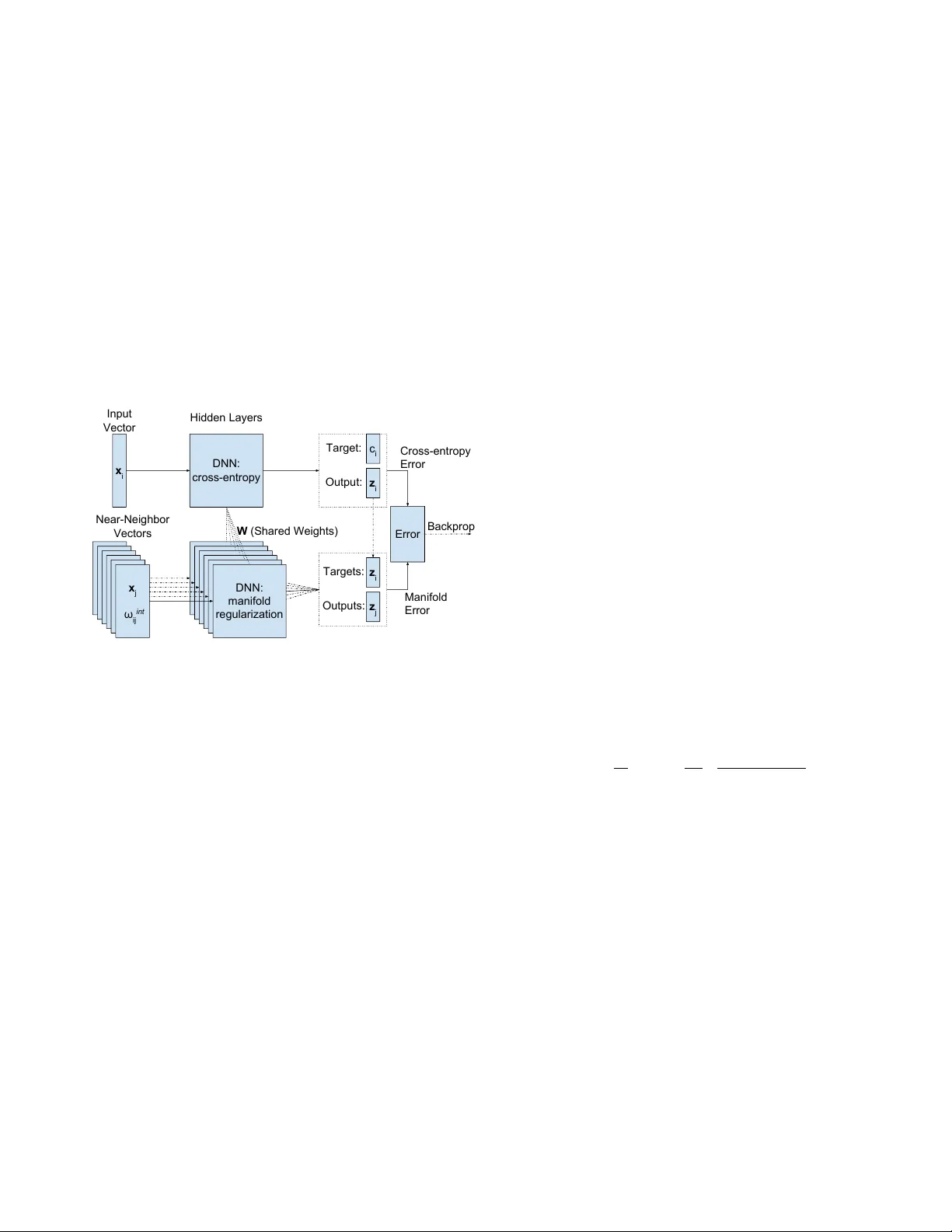
GRAPH B ASED MANIFOLD REGULARIZED DEEP NEURAL NETWORKS FOR A UT OMA TIC SPEECH RECOGNITION V ikrant Singh T omar 1 , 2 , Richar d Rose 1 , 3 1 McGill Uni versity , Department of Electrical and Computer Engineering, Montreal, Canada 2 Fluent.ai, Montreal, QC, Canada 3 Google Inc., NYC, USA ABSTRA CT Deep neural networks (DNNs) ha ve been successfully applied to a wide variety of acoustic modeling tasks in recent years. These include the applications of DNNs either in a discrim- inativ e feature extraction or in a hybrid acoustic modeling scenario. Despite the rapid progress in this area, a number of challenges remain in training DNNs. This paper presents an effecti ve way of training DNNs using a manifold learning based regularization framework. In this framework, the pa- rameters of the network are optimized to preserve underlying manifold based relationships between speech feature vectors while minimizing a measure of loss between netw ork outputs and tar gets. This is achieved by incorporating manifold based locality constraints in the objective criterion of DNNs. Em- pirical evidence is provided to demonstrate that training a net- work with manifold constraints preserves structural compact- ness in the hidden layers of the network. Manifold re gulariza- tion is applied to train bottleneck DNNs for feature e xtraction in hidden Marko v model (HMM) based speech recognition. The experiments in this work are conducted on the Aurora- 2 spoken digits and the Aurora-4 read news large vocab u- lary continuous speech recognition tasks. The performance is measured in terms of word error rate (WER) on these tasks. It is sho wn that the manifold regularized DNNs result in up to 37% reduction in WER relativ e to standard DNNs. Index T erms — manifold learning, deep neural networks, manifold regularization, manifold regularized deep neural networks, speech recognition 1. INTRODUCTION Recently there has been a resur gence of research in the area of deep neural networks (DNNs) for acoustic modeling in auto- matic speech recognition (ASR) [1–6]. Much of this research has been concentrated on techniques for regularization of the algorithms used for DNN parameter estimation [7 – 9]. At the same time, there has also been a great deal of research on graph based techniques that facilitate the preservation of lo- cal neighborhood relationships among feature vectors for pa- rameter estimation in a number of application areas [10–13]. Algorithms that preserve these local relationships are often referred to as having the ef fect of applying manifold based constraints. This is because subspace manifolds are generally defined to be low-dimensional, perhaps nonlinear , surfaces where locally linear relationships exist among points along the surface. Hence, preservation of these local neighborhood relationships is often thought, to some approximation, to have the effect of preserving the structure of the manifold. T o the extent that this assumption is correct, it suggests that the man- ifold shape can be preserv ed without knowledge of the overall manifold structure. This paper presents an approach for applying manifold based constraints to the problem of regularizing training al- gorithms for DNN based acoustic models in ASR. This ap- proach in volv es redefining the optimization criterion in DNN training to incorporate the local neighborhood relationships among acoustic feature vectors. T o this end, this work uses discriminativ e manifold learning (DML) based constraints. The resultant training mechanism is referred to here as mani- fold regularized DNN (MRDNN) training and is described in Section 3. Results are presented demonstrating the impact of MRDNN training on both the ASR word error rates (WERs) obtained from MRDNN trained models and on the behavior of the associated nonlinear feature space mapping. Previous work in optimizing deep network training in- cludes approaches for pre-training of network parameters such as restricted Boltzmann machine (RBM) based genera- tiv e pre-training [14–16], layer-by-layer discriminati ve pre- training [17], and stack ed auto-encoder based pre-training [18, 19]. Ho we ver , more recent studies have shown that, if there are enough observation vectors a vailable for training models, the network pre-training has little impact on ASR perfor- mance [6, 9]. Other techniques, like dropout with the use of rectified linear units (ReLUs) as nonlinear elements in place of sigmoid units in the hidden layers of the network are also thought to have the effect of regularization on DNN training [7, 8]. The manifold regularization techniques described in this paper are applied to estimate parameters for a tandem DNN with a low-dimensional bottleneck hidden layer [20]. The discriminativ e features obtained from the bottleneck layer are input to a Gaussian mixture model (GMM) based HMM (GMM-HMM) speech recognizer [4, 21]. This work ex- tends [22] by presenting an impro ved MRDNN training algo- rithm that results in reduced computational complexity and better ASR performance. ASR performance of the proposed technique is ev aluated on two well known speech-in-noise corpora. The first is the Aurora-2 speech corpus, a connected digit task [23], and the second is the Aurora-4 speech c orpus, a read news large vocabulary continuous speech recognition (L VCSR) task [24]. Both speech corpora and the ASR sys- tems configured for these corpora are described in Section 4. An important impact of the proposed technique is the well-behav ed internal feature representations associated with MRDNN trained networks. It is observed that the modified objectiv e criterion results in a feature space in the internal network layers such that the local neighborhood relationships between feature vectors are preserved. That is, if two input vectors, x i and x j , lie within the same local neighborhood in the input space, then their corresponding mappings, z i and z j , in the internal layers will also be neighbors. This prop- erty can be characterized by means of an objective measure referred to as the contraction ratio [25], which describes the relationship between the sizes of the local neighborhoods in the input and the mapped feature spaces. The performance of MRDNN training in producing mappings that preserve these local neighborhood relationships is presented in terms of the measured contraction ratio in Section 3. The locality preservation constraints associated with the MRDNN training are also shown in Section 3 to lead to a more robust gradient estimation in error back propagation training. The rest of this paper is structured as follows. Second 2 provides a revie w of basic principals associated with DNN training, manifold learning, and manifold re gularization. Sec- tion 3 describes the MRDNN algorithm formulation, and pro- vides a discussion of the contraction ratio as a measure of locality preserv ation in the DNN. Section 4 describes the task domains, system configurations and presents the ASR WER performance results. Section 5 discusses computational com- plexity of the proposed MRDNN training and the effect of noise on the manifold learning methods. In Section 5.3, an- other way of applying the manifold regularization to DNN training is discussed, where a manifold regularization is used only for first few training epochs. Conclusions and sugges- tions for future work are presented in Section 6. 2. BA CKGROUND This section provides a brief revie w of DNNs and manifold learning principals as context for the MRDNN approach pre- sented in Section 3. Section 2.1 provides a summary of DNNs and their applications in ASR. An introduction to manifold learning and related techniques is provided in Section 2.2; this includes the discriminativ e manifold learning (DML) frame- work and locality sensitiv e hashing techniques for speeding up the neighborhood search for these methods. Section 2.3 briefly describes the manifold regularization frame work and some of its example implementations. 2.1. Deep Neural Networks A DNN is simply a feed-forward artificial neural network that has multiple hidden layers between the input and out- put layers. T ypically , such a network produces a mapping f dnn : x → z from the inputs, x i , i = 1 . . . N , to the output activ ations, z i , i = 1 . . . N . This is achiev ed by finding an optimal set of weights, W , to minimize a global error or loss measure, V ( x i , t i , f dnn ) , defined between the outputs of the network and the targets, t i , i = 1 . . . N . In this work, L 2 - norm regularized DNNs are used as baseline DNN models. The objectiv e criterion for such a model is defined as F ( W ) = 1 N N X i =1 V ( x i , t i , f dnn ) + γ 1 || W || 2 , (1) where the second term refers to the L 2 -norm regularization applied to the weights of the network, and γ 1 is the regular - ization coef ficient that controls the relative contributions of the two terms. The weights of the network are updated for se veral epochs ov er the training set using mini-batch gradient descent based error back-propagation (EBP), w l m,n ← − w l m,n + η ∇ w l m,n F ( W ) , (2) where w l m,n refers to the weight on the input to the n th unit in the l th layer of the network from the m th unit in the pre- ceding layer . The parameter η corresponds to the gradient learning rate. The gradient of the global error with respect to w l m,n is giv en as ∇ w l m,n F ( W ) = − ∆ l m,n − 2 γ 1 w l m,n , (3) where ∆ l m,n is the error signal in the l th layer and its form depends on both the error function and the acti vation function. T ypically , a soft-max nonlinearity is used at the output layer along with the cross-entropy objective criterion. Assuming that the input to p th unit in the final layer is calculated as net L p = P n w L n,p z L − 1 p , the error signal for this case is gi ven as ∆ L n,p = ( z p − t p ) z L − 1 n [26, 27]. 2.2. Manifold Learning Manifold learning techniques work under the assumption that high-dimensional data can be considered as a set of ge- ometrically related points lying on or close to the surface of a smooth lo w dimensional manifold [12, 28, 29]. T ypi- cally , these techniques are used for dimensionality reducing feature space transformations with the goal of preserving manifold domain relationships among data vectors in the original space [28, 30]. The application of manifold learning methods to ASR is supported by the argument that speech is produced by the mov ements of loosely constrained articulators [13, 31]. Moti- vated by this, manifold learning can be used in acoustic mod- eling and feature space transformation techniques to preserve the local relationships between feature vectors. This can be realized by embedding the feature vectors into one or more partially connected graphs [32]. An optimality criterion is then formulated based on the preservation of manifold based geometrical relationships. One such example is locality pre- serving projections (LPP) for feature space transformations in ASR [33]. The objective function in LPP is formulated so that feature vectors close to each other in the original space are also close to each other in the target space. 2.2.1. Discriminative Manifold Learning Most manifold learning techniques are unsupervised and non-discriminativ e, for e xample, LPP . As a result, these tech- niques do not generally exploit the underlying inter-class discriminativ e structure in speech features. For this reason, features belonging to different classes might not be well sep- arated in the tar get space. A discriminativ e manifold learning (DML) framework for feature space transformations in ASR is proposed in [10, 34, 35]. The DML techniques incorpo- rate discriminative training into manifold based nonlinear locality preserv ation. For a dimensionality reducing mapping f G : x ∈ R D → z ∈ R d , where d << D , these techniques attempt to preserve the within class manifold based rela- tionships in the original space while maximizing a criterion related to the separability between classes in the output space. In DML, the manifold based relationships between the feature vectors are characterized by two separate partially connected graphs, namely intrinsic and penalty graphs [10, 32]. If the feature vectors, X ∈ R N × D , are represented by the nodes of the graphs, the intrinsic graph, G int = { X , Ω int } , characterizes the within class or within manifold relationships between feature vectors. The penalty graph, G pen = { X , Ω pen } , characterizes the relationships between feature vectors belonging to different speech classes. Ω int and Ω pen are known as the affinity matrices for the intrinsic and penalty graphs respectiv ely and represent the manifold based distances or weights on the edges connecting the nodes of the graphs. The elements of these affinity matrices are defined in terms of Gaussian kernels as ω int ij =    exp  −|| x i − x j || 2 ρ  ; C ( x i ) = C ( x j ) , e ( x i , x j ) = 1 0 ; Otherwise (4) and ω pen ij =    exp  −|| x i − x j || 2 ρ  ; C ( x i ) 6 = C ( x j ) , e ( x i , x j ) = 1 0 ; Otherwise , (5) where C ( x i ) refers to the class or label associated with v ector x i and ρ is the Gaussian kernel heat parameter . The function e ( x i , x j ) indicates whether x j is in the neighborhood of x i . Neighborhood relationships between two vectors can be de- termined by k -nearest neighborhood (kNN) search. In order to design an objecti ve criterion that minimizes manifold domain distances between feature vectors belong- ing to the same speech class while maximizing the distances between feature v ectors belonging to different speech classes, a graph scatter measure is defined. This measure represents the spread of the graph or average distance between feature vectors in the target space with respect to the original space. For a generic graph G = { X , Ω } , a measure of the graph’ s scatter for a mapping f G : x → z can be defined as F G ( Z ) = X i,j || z i − z j || 2 ω ij . (6) The objective criterion in discriminativ e manifold learning is designed as the difference of the intrinsic and penalty scatter measures, F G dif f ( Z ) = X i,j || z i − z j || 2 ω int ij − X i,j || z i − z j || 2 ω pen ij , = X i,j || z i − z j || 2 ω dif f ij , (7) where ω dif f ij = ω int ij − ω pen ij . DML based dimensionality reducing feature space trans- formation techniques hav e been reported to provide signifi- cant gains over con ventional techniques such as linear dis- criminant analysis (LD A) and unsupervised manifold learn- ing based LPP for ASR [10, 34, 35]. This has motiv ated the use of DML based constraints for regularizing DNNs in this work. 2.2.2. Locality Sensitive Hashing One key challenge in applying manifold learning based meth- ods to ASR is that due to large computational complexity requirements, these methods do not directly scale to big datasets. This complexity originates from the need to calcu- late a pair -wise similarity measure between feature v ectors to construct neighborhood graphs. This work uses locality sen- sitiv e hashing (LSH) based methods for fast construction of the neighborhood graphs as described in [36, 37]. LSH creates hashed signatures of vectors in order to distribute them into a number of discrete buckets such that vectors close to each other are more likely to fall into the same b ucket [38, 39]. In this manner, one can efficiently perform similarity searches by exploring only the data-points falling into the same or adjacent buck ets. 2.3. Manifold Regularization Manifold regularization is a data dependent regularization framew ork that is capable of exploiting the existing mani- fold based structure of the data distribution. It is introduced in [11], where the authors hav e also presented manifold extended versions of regularized least squares and support vector machines algorithms for a number of text and image classification tasks. There has been se veral recent ef forts to incorporate some form of manifold based learning into a variety of machine learning tasks. In [40], authors have in v estigated manifold regularization in single hidden layer multilayer perceptrons for a phone classification task. Manifold learning based semi- supervised embedding ha ve been applied to deep learning for a hand-written character recognition task in [41]. Manifold regularized single-layer neural networks hav e been used for image classification in [42]. In spite of these efforts of apply- ing manifold regularization to various application domains, similar efforts are not known for training deep models in ASR. 3. MANIFOLD REGULARIZED DEEP NEURAL NETWORKS The multi-layered nonlinear structure of DNNs makes them capable of learning the highly nonlinear relationships be- tween speech feature vectors. This section proposes an ex- tension of EBP based DNN training by incorporating the DML based constraints discussed in Section 2.2.1 as a re g- ularization term. The algorithm formulation is provided in Section 3.1. The proposed training procedure emphasizes local relationships among speech feature vectors along a low dimensional manifold while optimizing network parameters. T o support this claim, empirical e vidence is provided in Sec- tion 3.3 that a network trained with manifold constraints has a higher capability of preserving the local relationships between the feature vectors than one trained without these constraints. 3.1. Manifold Regularized T raining This work incorporates locality and geometrical relationships preserving manifold constraints as a regularization term in the objective criterion of a deep network. These constraints are deriv ed from a graph characterizing the underlying man- ifold of speech feature vectors in the input space. The ob- jectiv e criterion for a MRDNN network producing a mapping f mrdnn : x → z is giv en as follo ws, F ( W ; Z ) = N X i =1    1 N V ( x i , t i , f mrdnn ) + γ 1 || W || 2 + γ 2 1 k 2 k X j =1 || z i − z j || 2 ω int ij    , (8) where V ( x i , t i , f mrdnn ) is the loss between a tar get vector t i and output vector z i giv en an input vector x i ; V( · ) is taken to be the cross-entropy loss in this work. W is the matrix representing the weights of the network. The sec- ond term in Eq. (8) is the L 2 -norm regularization penalty on the network weights; this h elps in maintaining smooth- ness for the assumed continuity of the source space. The effect of this regularizer is controlled by the multiplier γ 1 . The third term in Eq. (8) represents manifold learning based locality preservation constraints as defined in Section 2.2.1. Note that only the constraints modeled by the intrinsic graph, G int = { X , Ω int } , are included, and the constraints mod- eled by the penalty graph, G pen = { X , Ω pen } , are ignored. This is further discussed in Section 3.2. The scalar k denotes the number of nearest neighbors connected to each feature vector , and ω int ij refers to the weights on the edges of the intrinsic graph as defined in Eq. (4). The relati ve impor- tance of the mapping along the manifold is controlled by the regularization coef ficient γ 2 . This framework assumes that the data distribution is sup- ported on a lo w dimensional manifold and corresponds to a data-dependent regularization that exploits the underlying manifold domain geometry of the input distribution. By im- posing manifold based locality preserving constraints on the network outputs in Eq. (8), this procedure encourages a map- ping where relationships along the manifold are preserved and different speech classes are well separated. The manifold reg- ularization term penalizes the objecti ve criterion for vectors that belong to the same neighborhood in the input space but hav e become separated in the output space after projection. The objectiv e criterion given in Eq. (8) has a very similar form to that of a standard DNN given in Eq. (1). The weights of the netw ork are optimized using EBP and gradient descent, ∇ W F ( W ; Z ) = N X i ∂ F ( W ; Z ) ∂ z i ∂ z i ∂ W , (9) where ∇ W F ( W ; Z ) is the gradient of the objective crite- rion with respect to the DNN weight matrix W . Using the same nomenclature as defined in Eq. (3), the gradient with respect to the weights in the last layer is calculated as ∇ w L n,p F ( W ; Z ) = − ∆ L n,p − 2 γ 1 w L n,p − 2 γ 2 k 2 k X j =1 ω ij ( z ( i ) ,p − z ( j ) ,p ) ∂ z ( i ) ,p ∂ w L n,p − ∂ z ( j ) ,p ∂ w L n,p ! , (10) where z ( i ) ,p refers to the activ ation of the p th unit in the out- put layer when the input vector is x i . The error signal, ∆ L n,p , is the same as the one specified in Eq. (3). 3.2. Architecture and Implementation The computation of the gradient in Eq. (10) depends not only on the input vector , x i , but also its neighbors, x j , j = 1 , . . . , k , that belong to the same class. Therefore, MRDNN training can be broken down into tw o components. The first is the standard DNN component that minimizes a cross-entropy based error with respect to giv en targets. The second is the manifold regularization based component that focuses on pe- nalizing a criterion related to preservation of neighborhood relationships. An architecture for manifold regularized DNN training is shown in Figure 1. For each input feature vector , x i , k of its nearest neighbors, x j , j = 1 , . . . , k , belonging to the same class are selected. These k + 1 vectors are forward propa- gated through the network. This can be visualized as making k + 1 separate copies of the DNN one for the input v ector and the remaining k for its neighbors. The DNN corresponding to the input vector , x i , is trained to minimize cross-entropy error with respect to a giv en target, t i . Each copy-DNN cor- responding to one of the selected neighbors, x j , is trained to minimize a function of the distance between its output, z j , and that corresponding to the input vector , z i . Note that the weights of all these copies are shared, and only an av erage gradient is used for weight-update. This algorithm is then e x- tended for use in mini-batch training. Hidden Layers W (Shared Weights) x j , ω ij int DNN (manifold regularization) x j , ω ij int DNN (manifold regularization) x j , ω ij int DNN (manifold regularization) x j , ω ij int DNN (manifold regularization) x j , ω ij int DNN (manifold regularization) x j ω ij int DNN: manifold regularization x i DNN: cross-entropy Error Backprop Input Vector Targets: z i z j Outputs: Target: c i z i Output: Near-Neighbor Vectors Cross-entropy Error Manifold Error Fig. 1 . Illustration of MRDNN architecture. For each input vector , x i , k of its neighbors, x j , belonging to the same class are selected and forw ard propagated through the netw ork. For the neighbors, the target is set to be the output vector corre- sponding to x i . The scalar ω int ij represents the intrinsic af fin- ity weights as defined in Eq. (4). It should be clear from this discussion that the relation- ships between a gi ven vector and its neighbors play an impor - tant role in the weight update using EBP . Giv en the assump- tion of a smooth manifold, the graph based manifold regular - ization is equiv alent to penalizing rapid changes of the clas- sification function. This results in smoothing of the gradient learning curve that leads to robust computation of the weight updates. In the applications of DML framew ork for feature space transformations, inclusion of both the intrinsic and penalty graphs terms, as shown in Eq. (7), is found to be important [10, 34, 43]. For this reason, experiments in the previous work included both these terms [22]. Howe ver , in initial experi- ments performed on the corpora described in Section 4, the gains achie ved by including the penalty graph were found to be inconsistent across datasets and different noise conditions. This may be because adding an additional term for discrimi- nating between classes of speech feature vectors might not al- ways impact the performance of DNNs since DNNs are inher- ently powerful discriminativ e models. Therefore, the penalty graph based term is not included in any of the experiments presented in this work, and the manifold learning based ex- pression given in Eq. (8) consists of the intrinsic component only . 3.3. Preserving Neighborhood Relationships This section describes a study conducted to characterize the effect of applying manifold based constraints on the beha vior of a deep network. This is an attempt to quantify how neigh- borhood relationships between feature vectors are preserved within the hidden layers of a manifold regularized DNN. T o this end, a measure referred to as the contraction ratio is in- vestigated. A form of this measure is presented in [25]. In this work, the contraction ratio is defined as the ratio of distance between two feature vectors at the output of the first hidden layer to that at the input of the network. The av erage contraction ratio between a feature vector and its neighbors can be seen as a measure of locality preservation and com- pactness of its neighborhood. Thus, the ev olution of the av- erage contraction ratio for a set of vectors as a function of distances between them can be used to characterize the over - all locality preserving behavior of a network. T o this end, a subset of feature vectors not seen during the training are se- lected. The distrib ution of pair-wise distances for the selected vectors is used to identify a number of bins. The edges of these bins are treated as a range of radii around the feature vectors. An av erage contraction ratio is computed as a func- tion of radius in a range r 1 < r ≤ r 2 ov er all the selected vectors and their neighbors falling in that range as C R ( r 1 , r 2 ) = 1 N N X i =1 X j ∈ Φ 1 k Φ · || z 1 i − z 1 j || 2 || x i − x j || 2 , (11) where for a giv en vector x i , Φ represents a set of vectors x j such that r 2 1 < || x i − x j || 2 ≤ r 2 2 , and k Φ is the number of such vectors. z 1 i represents the output of the first layer cor- responding to vector x i at the input. It follows that a smaller contraction ratio represents a more compact neighborhood. Figure 2 displays the contraction ratio of the output to in- put neighborhood sizes relativ e to the radius of the neighbor- hood in the input space for the DNN and MRDNN systems. The av erage contraction ratios between the input and the first layer’ s output features are plotted as functions of the median radius of the bins. It can be seen from the plots that the features obtained from a MRDNN represent a more compact neighborhood than those obtained from a DNN. Therefore it can be concluded that the hidden layers of a MRDNN are able to learn the manifold based local geometrical representation of the feature space. It should also be noted that the contrac- tion ratio increases with the radius indicating that the effect of Input Neighborhood Radius 0 20 40 60 80 100 Contraction Ratio 0.6 0.7 0.8 0.9 1 1.1 1.2 1.3 DNN MRDNN Fig. 2 . Contraction ratio of the output to input neighborhood sizes as a function of input neighborhood radius. manifold preservation diminishes as one moves farther from a giv en vector . This is in agreement with the local in variance assumption ov er low-dimensional manifolds. 4. EXPERIMENT AL STUDY This section presents the experimental study conducted to ev aluate the ef fecti veness of the proposed MRDNNs in terms of ASR WER. The ASR performance of a MRDNN is pre- sented and compared with that of DNNs without manifold regularization and the traditional GMM-HMM systems. The experiments in this work are done on two separate speech- in-noise tasks, namely the Aurora-2, which is a connected digit task, and the Aurora-4, which is a read news L VCSR task. The speech tasks and the system setup are described in Section 4.1. The results of the experiments on the Aurora-2 task are presented in Section 4.2. The results and compara- tiv e performance of the proposed technique on the Aurora-4 task are presented in Section 4.3. In addition, experiments on clean condition training sets of the Aurora-2 and Aurora-4 are also performed. The results for these experiments are provided in Section 4.4. 4.1. T ask Domain and System Configuration The first dataset used in this work is the Aurora-2 connected digit speech in noise corpus. In most of the experiments, the Aurora-2 mixed-condition training set is used for train- ing [23]. Some experiments hav e also used the clean training set. Both the clean and mixed-conditions training sets contain a total of 8440 utterances by 55 male and 55 female speak- ers. In the mixed-conditions set, the utterances are corrupted by adding four different noise types to the clean utterances. The con ventional GMM-HMM ASR system is configured us- ing the standard configuration specified in [23]. This corre- sponds to using 10 word-based continuous density HMMs (CDHMMs) for digits 0 to 9 with 16 states per word-model, and additional models with 3 states for silence and 1 state for short-pause. In total, there are 180 CDHMM states each modeled by a mix of 3 Gaussians. During the test phase, fiv e different subsets are used corresponding to uncorrupted clean utterances and utterances corrupted with four differ - ent noise types, namely subway , babble, car and exhibition hall, at signal-to-noise ratios (SNRs) ranging from 5 to 20 dB. There are 1001 utterances in each subset. The ASR per- formance obtained for the GMM-HMM system configuration agrees with those reported elsewhere [23]. The second dataset used in this work is the Aurora-4 read newspaper speech-in-noise corpus. This corpus is created by adding noise to the W all Street Journal corpus [24]. Aurora- 4 represents a MVCSR task with a vocab ulary size of 5000 words. This work uses the standard 16kHz mixed-conditions training set of the Aurora-4 [24]. It consists of 7138 noisy utterances from a total of 83 male and female speakers corre- sponding to about 14 hours of speech. One half of the utter- ances in the mixed-conditions training set are recorded with a primary Sennheiser microphone and the other half with a secondary microphone, which enables the effect of transmis- sion channel. Both halves contain a mixture of uncorrupted clean utterances and noise corrupted utterances with the SNR lev els varying from 10 to 20 dB in 6 dif ferent noise condi- tions (babble, street traf fic, train station, car, restaurant and airport). A bi-gram language model is used with a perplex- ity of 147. Context-depedent cross-word triphone CDHMM models are used for configuring the ASR system. There are a total of 3202 senones and each state is modeled by 16 Gaus- sian components. Similar to the training set, the test set is recorded with the primary and secondary microphones. Each subset is further divided into sev en subsets, where one sub- set is clean speech data and the remaining six are obtained by randomly adding the same six noise types as training at SNR lev els ranging from 5 to 15 dB. Thus, there are a total of 14 subsets. Each subset contains 330 utterances from 8 speak ers. It should be noted that both of the corpora used in this work represent simulated speech-in-noise tasks. These are created by adding noises from multiple sources to speech ut- terances spoken in a quite en vironment. For this reason, one should be careful about generalizing these results to other speech-in-noise tasks. For both corpora, the baseline GMM-HMM ASR systems are configured using 12-dimensional static Mel-frequency cepstrum coef ficient (MFCC) features augmented by normal- ized log energy , difference cepstrum, and second difference cepstrum resulting in 39-dimensional vectors. The ASR per- formance is reported in terms of WERs. These GMM-HMM systems are also used for generating the context-dependent state alignments. These alignments are then used as the tar get labels for deep networks training as described belo w . Collectiv ely , the term “deep network” is used to refer to both DNN and MRDNN configurations. Both of these configurations include L 2 -norm regularization applied to the weights of the networks. The ASR performance of these models is evaluated in a tandem setup where a bottleneck deep network is used as feature extractor for a GMM-HMM system. The deep networks take 429-dimensional input vec- tors that are created by concatenating 11 context frames of 12-dimensional MFCC features augmented with log energy , and first and second order difference. The number of units in the output layer is equal to the number of CDHMM states. The class labels or targets at the output are set to be the CDHMM states obtained by a single pass force-alignment using the baseline GMM-HMM system. The regularization coefficient γ 1 for the L 2 weight decay is set to 0.0001. In the MRDNN setup, the number of nearest neighbors, k , is set to 10, and γ 2 is set to 0.001. While the manifold regularization techniques is not ev aluated for hybrid DNN-HMM systems, one would expect the presented results to generalize to those models. The experimental study performed in this work is limited to tandem DNN-HMM scenarios. It is expected that the results reported here should also generalize to DNN train- ing for hybrid DNN-HMM configurations. This is a topic for future work. For the Aurora-2 experiments, the deep networks have fiv e hidden layers. The first four hidden layers have 1024 hid- den units each, and the fifth layer is bottleneck layer with 40 hidden units. For the Aurora-4 experiments, larger networks are used. There are sev en hidden layers. The first six hidden layers hav e 2048 hidden units each, and the seventh layer is bottleneck layer with 40 hidden units. This lar ger network for Aurora-4 is in-line with other recent work [44, 45]. The hid- den units use ReLUs as activ ation functions. The soft-max nonlinearity is used in the output layer with the cross-entropy loss between the outputs and targets of the network as the error [26, 27]. After the EBP training, the 40-dimensional output features are taken from the bottleneck layer and de- correlated using principal component analysis (PCA). Only features corresponding to the top 39 components are kept dur - ing the PCA transformation to match the dimensionality of the baseline system. The resultant features are used to train a GMM-HMM ASR system using a maximum-likelihood cri- terion. Although some might ar gue that PCA is not neces- sary after the compressed bottleneck output, in this work, a performance gain of 2-3% absolute is observed with PCA on the same bottleneck features for different noise and channel conditions. No difference in performance is observed for the clean data. 4.2. Results for the mixed-noise A urora-2 Spoken Digits Corpus The ASR WER for the Aurora-2 speech-in-noise task are pre- sented in T able 1. The models are trained on the mixed-noise T able 1 . WERs for mixed noise training and noisy test- ing on the Aurora-2 speech corpus for GMM-HMM, DNN and MRDNN systems. The best performance has been high- lighted for each noise type per SNR lev el. Noise T echnique SNR (dB) 20 15 10 5 Subway GMM-HMM 2.99 4.00 6.21 11.89 DNN 1.19 1.69 2.95 6.02 MRDNN 0.91 1.60 2.39 5.67 Babble GMM-HMM 3.31 4.37 7.97 18.06 DNN 1.15 1.42 2.81 7.38 MRDNN 0.83 1.26 2.27 7.05 Car GMM-HMM 2.77 3.36 5.45 12.31 DNN 1.05 1.85 2.98 6.92 MRDNN 0.84 1.37 2.59 6.38 Exhibition GMM-HMM 3.34 3.83 6.64 12.72 DNN 1.23 1.54 3.30 7.87 MRDNN 0.96 1.44 2.48 7.24 set. The test results are presented in four separate tables each corresponding to a dif ferent noisy subset of the Aurora-2 test set. Each noisy subset is further di vided into four subsets corresponding to noise corrupted utterances with 20 to 5dB SNRs. For each noise condition, the ASR results for features obtained from three dif ferent techniques are compared. The first row of each table, labeled ‘GMM-HMM’, contains the ASR WER for the baseline GMM-HMM system trained us- ing MFCC features appended with first and second order dif- ferences. The second row , labeled ‘DNN’, displays results for the bottleneck features taken from the DNN described in Section 2.1. The final row , labeled ‘MRDNN’, presents the ASR WER results for the bottleneck features obtained from the MRDNN described in Section 3.1. For all the cases, the GMM-HMM and DNN configurations described in Section 4.1 are used. The initial learning rates for both systems are set to 0.001 and decreased exponentially with each epoch. Each system is trained for 40 epochs ov er the training set. T wo main observations can be made from the results pre- sented in T able 1. First, both DNN and MRDNN provide sig- nificant reductions in ASR WER over the GMM-HMM sys- tem. The second observation can be made by comparing the ASR performance of DNN and MRDNN systems. It is evi- dent from the results presented that the features derived from a manifold regularized network pro vide consistent gains over those deri ved from a network that is re gularized only with the L 2 weight-decay . The maximum relativ e WER gain obtained by using MRDNN ov er DNN is 37%. 4.3. Results for the mixed-noise A urora-4 Read News Corpus The ASR WERs for the Aurora-4 task are gi ven in T able 2. All three acoustic models in the table are trained on the T able 2 . WER for mix ed conditions training on the Aurora-4 task for GMM-HMM, DNN, and MRDNN systems. Clean Noise Channel Noise + Channel GMM-HMM 13.02 18.62 20.27 30.11 DNN 5.91 10.32 11.35 22.78 MRDNN 5.30 9.50 10.11 21.90 Aurora-4 mixed-conditions set. The table lists ASR WERs for four sets, namely clean, additive noise (noise), channel distortion (channel), and additive noise combined with chan- nel distortion (noise + channel). These sets are obtained by grouping together the fourteen subsets described in Section 4.1. The first row of the table, labeled ‘GMM-HMM’, pro- vides results for the traditional GMM-HMM system trained using MFCC features appended with first and second order differences. The second row , labeled ‘DNN’, presents WERs corresponding to the features derived from the baseline L 2 regularized DNN system. ASR performances for the base- line systems reported in this work agree with those reported elsewhere [44, 45]. The baseline set-up is consistent with that specified for the Aurora 4 task in order to be able to make comparisons with other results obtained in the literature for that task. The third row , labeled ‘MRDNN’, displays the WERs for features obtained from a MRDNN. Similar to the case for Aurora-2, L2 regularization with the coef ficient γ 1 set to 0.0001 is used for training both the DNN and MRDNN. The initial learning rate is set to 0.003 and reduced exponen- tially for 40 epochs when the training is stopped. Similar to the results for the Aurora-2 corpus, two main observations can be made by comparing the performance of the presented systems. First, both DNN and MRDNN pro- vide large reductions in WERs over the GMM-HMM for all conditions. Second, the trend of the WER reductions by us- ing MRDNN ov er DNN is visible here as well. The max- imum relati ve WER reduction obtained by using MRDNN ov er DNN is 10.3%. The relati ve gain in the ASR performance for the Aurora- 4 corpus is less than that for the Aurora-2 corpus. This might be due to the fact that the performance of manifold learn- ing based algorithms is highly susceptible to the presence of noise. This increased sensitivity is linked to the Gaussian ker - nel scale factor , ρ , defined in Eq. (4) [43]. In this work, ρ , is set to be equal to 1000 for all the experiments. This value is taken from previous work where it is empirically derived on a subset of Aurora-2 for a different task [34, 43]. While it is easy to analyze the effect of noise on the performance of the discussed models at each SNR lev el for the Aurora-2 corpus, it is difficult to do the same for the Aurora-4 corpus because of the way the corpus is organized. The Aurora-4 corpus only provides a mixture of utterances at different SNR lev els for each noise type. Therefore, the average WER giv en for the Aurora-4 corpus might be affected by the dependence of ASR performance on the choice of ρ and SNR levels, and a better tuned model is e xpected to provide improved performance. This is further discussed in Section 5.2. Note that other techniques that hav e been reported to pro- vide gains for DNNs were also in vestigated in this work. In particular , the use of RBM based generativ e pre-training was in vestigated to initialize the weights of the DNN system. Sur- prisingly , ho we ver , the generative pre-training mechanism did not lead to an y reductions in ASR WER performance on these corpora. This is in agreement with other recent studies in the literature, which have suggested that the use of ReLU hidden units on a relatively well-behav ed corpus with enough train- ing data obviates the need of a pre-training mechanism [9]. 4.4. Results for Clean-condition T raining In addition to the experiments on the mixed-conditions noisy datasets discussed in Sections 4.2 and 4.3, experiments are also conducted to e valuate the performance of MRDNN for matched clean training and testing scenarios. T o this end, the clean training sets of the Aurora-2 and Aurora-4 corpora are used for training the deep networks as well as building mani- fold based neighborhood graphs [23, 24]. The results are pre- sented in T able 3. It can be observed from the results pre- sented in the table that MRDNN provides 21.05% relativ e improv ements in WER ov er DNN for the Aurora-2 set and 14.43% relativ e improvement for the Aurora-4 corpus. T able 3 . WERs for clean training and clean testing on the Aurora-2 and Aurora-4 speech corpora for GMM-HMM, DNN, and MRDNN models. The last column lists % WER improv ements of MRDNN relativ e to DNN. GMM-HMM DNN MRDNN % Imp. Aurora-2 0.93 0.57 0.45 21.05 Aurora-4 11.87 8.11 6.94 14.43 The ASR performance results presented for the Aurora-2 and the Aurora-4 corpora in Sections 4.2, 4.3 and 4.4 demon- strate the effecti veness of the proposed manifold regularized training for deep networks. While the con ventional pre- training and regularization approaches did not lead to any performance gains, the MRDNN training provided consistent reductions in WERs. The primary reason for this perfor- mance gain is the ability of MRDNNs to learn and preserve the underlying lo w-dimensional manifold based relationships between feature vectors. This has been demonstrated with empirical evidence in Section 3.3. Therefore, the proposed MRDNN technique provides a compelling regularization scheme for training deep networks. 5. DISCUSSION AND ISSUES There are a number of factors that can have an impact on the performance and application of MRDNN to ASR tasks. This section highlights some of the factors and issues affect- ing these techniques. 5.1. Computational Complexity Though the inclusion of a manifold regularization factor in DNN training leads to encouraging gains in WER, it does so at the cost of additional computational complexity for param- eter estimation. This additional cost for MRDNN training is two-fold. The first is the cost associated with calculating the pair-wise distances for populating the intrinsic affinity matrix, Ω int . As discussed in Section 2.2.2 and [36, 37], this compu- tation complexity can be managed by using locality sensiti ve hashing for approximate nearest neighbor search without sac- rificing ASR performance. The second source of this additional complexity is the in- clusion of k neighbors for each feature v ector during forward and back propagation. This results in an increase in the com- putational cost by a factor of k . This cost can be managed by various parallelization techniques [3] and becomes ne gligible in the light of the massively parallel architectures of the mod- ern processing units. This added computational cost is only relvent during the training of the networks and has no impact during the test phase or when the data is transformed using a trained network. The networks in this work are training on Nvidia K20 graphics boards using tools developed on python based frame- works such as numpy , gnumpy and cudamat [46, 47]. For DNN training, each epoch over the Aurora-2 set took 240 seconds and each epoch over the Aurora-4 dataset took 480 seconds. In comparison, MRDNN training took 1220 sec- onds for each epoch over the Aurora-2 set and 3000 seconds for each epoch ov er the Aurora-4 set. 5.2. Effect of Noise In previous work, the authors hav e demonstrated that mani- fold learning techniques are very sensitiv e to the presence of noise [43]. This sensitivity can be traced to the Gaussian ker- nel scale factor , ρ , used for defining the local af finity matrices in Eq. (4). This argument might apply to MRDNN training as well. Therefore, the performance of a MRDNN might be affected by the presence of noise. This is visible to some ex- tent in the results presented in T able 1, where the WER gains by using MRDNN over DNN vary with SNR level. On the other hand, the Aurora-4 test corpus contains a mixture of noise corrupted utterances at different SNR lev els for each noise type. Therefore, only an average ov er all SNR le vels per noise type is presented. There is a need to conduct e xtensiv e experiments to in- vestigate this ef fect as was done in [43]. Howe ver , if these models are af fected by the presence of noise in a similar man- ner , additional gains could be derived by designing a method for building the intrinsic graphs separately for different noise T able 4 . A verage WERs for mixed noise training and noisy testing on the Aurora-2 speech corpus for DNN, MRDNN and MRDNN 10 models. Noise T echnique SNR (dB) clean 20 15 10 5 A vg. DNN 0.91 1.16 1.63 3.01 7.03 MRDNN 0.66 0.88 1.42 2.43 6.59 MRDNN 10 0.62 0.81 1.37 2.46 6.45 conditions. During the DNN training, an automated algorithm could select a graph that best matches the estimated noise con- ditions associated with a giv en utterance. Training in this way could result in a MRDNN that is able to pro vide further gains in ASR performance in various noise conditions. 5.3. Alternating Manifold Regularized T raining Section 4 has demonstrated reductions in ASR WER by forcing the output feature vectors to conform to the local neighborhood relationships present in the input data. This is achiev ed by applying the underlying input manifold based constraints to the DNN outputs throughout the training. There hav e also been studies in literature where manifold regular- ization is used only for first few iterations of model training. For instance, authors in [48] have applied manifold regular - ization to multi-task learning. The authors have argued that optimizing deep networks by alternating between training with and without manifold based constraints can increase the generalization capacity of the model. Motiv ated by these efforts, this section in vestigates a sce- nario in which the manifold regularization based constraints are used only for the first few epochs of the training. All lay- ers of the networks are randomly initialized and then trained with the manifold based constraints for first 10 epochs. The resultant network is then further trained for 20 epochs us- ing the standard EBP without manifold based regularization. Note that contrary to the pre-training approaches in deep learning, this is not a greedy layer-by-layer training. ASR results for these experiments are gi ven in T able 4 for the Aurora-2 dataset. For brevity , the table only presents the ASR WERs as an av erage o ver the four noise types described in T able 1 at each SNR le vel. In addition to the a verage WERs for the DNN and MRDNN, a ro w labeled ‘MRDNN 10’ is giv en. This row refers to the case where manifold regulariza- tion is used only for first 10 training epochs. A number of observations can be made from the results presented in T able 4. First, it can be seen from the results in T able 4 that both MRDNN and MRDNN 10 training sce- narios improv e ASR WERs when compared to the standard DNN training. Second, MRDNN 10 training provides further reductions in ASR WERs for the Aurora-2 set. Experiments on the clean training and clean testing set of the Aurora-2 corpus also results in interesting comparison. In this case, the MRDNN 10 training improved ASR performance to 0.39% WER as compared to 0.45% for MRDNN and 0.57% for DNN training. That translates to 31.5% gain in ASR WER relativ e to DNNs. The WER reductions achie ved in these experiements are encouraging. Furthermore, this approach where manifold constraints are applied only for the first few epochs might lead to a more efficient manifold regularized training procedure because manifold regularized training has higher computa- tional complexity than a DNN (as discussed in Section 5.1). Howe ver , unlike [48], this work only applied one cycle of manifold constrained-unconstrained training. It should be noted that these are preliminary experiments. Similar gains are not seen when these techniques are applied to the Aurora- 4 dataset. Therefore, further in vestigation is required before making any substantial conclusions. 6. CONCLUSIONS AND FUTURE WORK This paper has presented a framework for regularizing the training of DNNs using discriminative manifold learning based locality preserving constraints. The manifold based constraints are deriv ed from a graph characterizing the un- derlying manifold of the speech feature vectors. Empirical evidence has also been provided showing that the hidden layers of a MRDNN are able to learn the local neighbor- hood relationships between feature vectors. It has also been conjectured that the inclusion of a manifold regularization term in the objectiv e criterion of DNNs results in a robust computation of the error gradient and weight updates. It has been sho wn through experimental results that the MRDNNs result in consistent reductions in ASR WERs that range up to 37% relati ve to the standard DNNs on the Aurora- 2 corpus. For the Aurora-4 corpus, the WER gains range up to 10% relative on the mix ed-noise training and 14.43% on the clean training task. Therefore, the proposed manifold reg- ularization based training can be seen as a compelling regu- larization scheme. The studies presented here open a number of interesting possibilities. One would expect MRDNN training to have a similar impact in hybrid DNN-HMM systems. The applica- tion of these techniques in semi-supervised scenarios is also a topic of interest. T o this end, the manifold regulariz ation based techniques could be used for learning from a large un- labeled dataset, followed by fine-tuning on a smaller labeled set. Acknowledgements The authors thank Nuance Foundation for providing finan- cial support for this project. The e xperiments were conducted on the Calcul-Quebec and Compute-Canada supercomputing clusters. The authors are thankful to the consortium for pro- viding the access and support. 7. REFERENCES [1] Navdeep Jaitly , Patrick Nguyen, Andre w Senior , and V incent V anhoucke, “An application of pretrained deep neural networks to large vocabulary con versational speech recognition, ” in Interspeech , 2012, number Cd, pp. 3–6. [2] Geoffrey Hinton, Li Deng, and Dong Y u, “Deep neural networks for acoustic modeling in speech recognition, ” IEEE Signal Pr ocess. Mag. , pp. 1–27, 2012. [3] T ara N. Sainath, Brian Kingsbury , Bhuvana Ramabhad- ran, Petr Fousek, Petr Nov ak, and Abdel-Rahman Mo- hamed, “Making deep belief networks effecti ve for lar ge vocab ulary continuous speech recognition, ” in IEEE W ork. Autom. Speech Recognit. Underst. , Dec. 2011, pp. 30–35. [4] Z T ¨ uske, Martin Sundermeyer , R Schl ¨ uter , and Hermann Ney , “Conte xt-dependent MLPs for L VCSR: T AN- DEM, hybrid or both, ” in Interspeech , Portland, OR, USA, 2012. [5] Y oshua Bengio, “Deep learning of representations: Looking forward, ” Stat. Lang. Speech Pr ocess. , pp. 1– 37, 2013. [6] Li Deng, Geoffre y Hinton, and Brian Kingsbury , “New types of deep neural network learning for speech recog- nition and related applications: An ov erview, ” in Proc. ICASSP , 2013. [7] GE Dahl, TN Sainath, and GE Hinton, “Improving deep neural networks for L VCSR using rectified linear units and dropout, ” ICASSP , 2013. [8] MD Zeiler, M Ranzato, R Monga, and M Mao, “On Rectified Linear Units for Speech Processing, ” pp. 3–7, 2013. [9] Li Deng, Jinyu Li, JT Huang, Kaisheng Y ao, and Dong Y u, “Recent advances in deep learning for speech re- search at Microsoft, ” ICASSP 2013 , pp. 0–4, 2013. [10] V ikrant Singh T omar and Richard C Rose, “A family of discriminative manifold learning algorithms and their application to speech recognition, ” IEEE/ACM T rans. Audio, Speech Lang. Pr ocess. , vol. 22, no. 1, pp. 161– 171, 2014. [11] Mikhail Belkin, Partha Niyogi, and V ikas Sindhwani, “Manifold Regularization : A Geometric Framew ork for Learning from Labeled and Unlabeled Examples, ” J. Mach. Learn. , v ol. 1, pp. 1–36, 2006. [12] Xiaofei He and Partha Niyogi, “Locality preserving pro- jections, ” in Neural Inf. Process. Syst. , 2002. [13] Aren Jansen and Partha Niyogi, “Intrinsic Fourier analy- sis on the manifold of speech sounds, ” in ICASSP IEEE Int. Conf. Acoust. Speech Signal Pr ocess. , 2006. [14] GE Hinton, Simon Osindero, and YW T eh, “A fast learning algorithm for deep belief nets, ” Neural Com- put. , 2006. [15] Dong Y u, Li Deng, and George E Dahl, “Roles of pre-training and fine-tuning in context-dependent DBN- HMMs for real-world speech recognition, ” in NIPS W ork. Deep Learn. Unsupervised F eatur . Learn. , 2010. [16] GE Dahl, Dong Y u, Li Deng, and A Acero, “Context- dependent pre-trained deep neural networks for large vocab ulary speech recognition, ” IEEE T rans. Audio, Speech Lang. Process. , pp. 1–13, 2012. [17] Frank Seide, Gang Li, Xie Chen, and Dong Y u, “Feature engineering in context-dependent deep neural networks for con versational speech transcription, ” in IEEE W ork. Autom. Speech Recognit. Underst. , Dec. 2011, pp. 24– 29. [18] Pascal V incent, Hugo Larochelle, and Isabelle Lajoie, “Stacked denoising autoencoders: Learning useful rep- resentations in a deep network with a local denoising criterion, ” J. Mach. Learn. Res. , vol. 11, pp. 3371–3408, 2010. [19] Hugo Larochelle and Y oshua Bengio, “Exploring strate- gies for training deep neural networks, ” J. Mach. Learn. Res. , vol. 1, pp. 1–40, 2009. [20] F Gr ´ ezl and M Karafi ´ at, “Probabilistic and bottle-neck features for L VCSR of meetings, ” in Int. Conf. Acoust. Speech, Signal Pr ocess. , 2007. [21] Hynek Hermansky , Daniel Ellis, and Sangita Sharma, “T andem connectionist feature extraction for con ven- tional HMM systems, ” in ICASSP , 2000, pp. 1–4. [22] V ikrant Singh T omar and Richard C Rose, “Manifold Regularized Deep Neural Networks, ” in Interspeech , 2014. [23] HG Hirsch and David Pearce, “The Aurora experimen- tal framework for the performance e valuation of speech recognition systems under noisy conditions, ” in Autom. Speech Recognit. Challenges next millenium , 2000. [24] N. Parihar and Joseph Picone, “ Aurora W orking Group : DSR Front End L VCSR Ev aluation, ” T ech. Rep., Eu- ropean T elecommunications Standards Institute, 2002. [25] Salah Rifai, Pascal V incent, Xavier Muller , Glorot Xavier , and Y oshua Bengio, “Contracti ve auto-encoders : explicit inv ariance during feature extraction, ” in Int. Conf. Mach. Learn. , 2011, vol. 85, pp. 833–840. [26] RA Dunne and NA Campbell, “On the pairing of the Softmax activ ation and cross-entropy penalty functions and the deriv ation of the Softmax activ ation function, ” in Pr oc. 8th Aust. Conf. Neural Networks , 1997, pp. 1– 5. [27] P Golik, P Doetsch, and H Ney , “Cross-entropy vs. squared error training: a theoretical and experimental comparison., ” in Interspeec h , 2013, pp. 2–6. [28] JB T enenbaum, “Mapping a manifold of perceptual ob- servations, ” Adv . Neural Inf. Pr ocess. Syst. , 1998. [29] LK Saul and ST Roweis, “Think globally , fit locally: unsupervised learning of low dimensional manifolds, ” J. Mach. Learn. Res. , vol. 4, pp. 119–155, 2003. [30] M Liu, K Liu, and X Y e, “Find the intrinsic space for multiclass classification, ” A CM Proc. Int. Symp. Appl. Sci. Biomed. Commun. T echnol. (ACM ISABEL) , 2011. [31] Aren Jansen and Partha Niyogi, “A geometric per- spectiv e on speech sounds, ” T ech. Rep., University of Chicago, 2005. [32] Shuicheng Y an, Dong Xu, Benyu Zhang, Hong-Jiang Zhang, Qiang Y ang, and Stephen Lin, “Graph embed- ding and extensions: a general frame work for dimen- sionality reduction., ” IEEE T rans. P attern Anal. Mach. Intell. , vol. 29, no. 1, pp. 40–51, Jan. 2007. [33] Y un T ang and Richard Rose, “A study of using locality preserving projections for feature extraction in speech recognition, ” in IEEE Int. Conf. Acoust. Speech Sig- nal Pr ocess. , Las V egas, NV , Mar . 2008, pp. 1569–1572, IEEE. [34] V ikrant Singh T omar and Richard C Rose, “Application of a locality preserving discriminant analysis approach to ASR, ” in 2012 11th Int. Conf. Inf. Sci. Signal Pr ocess. their Appl. , Montreal, QC, Canada, July 2012, pp. 103– 107, IEEE. [35] V ikrant Singh T omar and Richard C Rose, “A correla- tional discriminant approach to feature extraction for ro- bust speech recognition, ” in Interspeech , Portland, OR, USA, 2012. [36] V ikrant Singh T omar and Richard C Rose, “Efficient manifold learning for speech recognition using locality sensitiv e hashing, ” in ICASSP IEEE Int. Conf. Acoust. Speech Signal Pr ocess. , V ancouver , BC, Canada, 2013. [37] V ikrant Singh T omar and Richard C Rose, “Locality sensitiv e hashing for fast computation of correlational manifold learning based feature space transformations, ” in Interspeech , L yon, France, 2013, pp. 2–6. [38] Piotr Indyk and R Motwani, “ Approximate nearest neighbors: to wards removing the curse of dimension- ality , ” in Pr oc. thirtieth Annu. ACM Symp. Theory Com- put. , 1998, pp. 604–613. [39] Mayur Datar , Nicole Immorlica, Piotr Indyk, and V a- hab S. Mirrokni, “Locality-sensitive hashing scheme based on p-stable distributions, ” Pr oc. T went. Annu. Symp. Comput. Geom. - SCG ’04 , p. 253, 2004. [40] Amarnag Subramanya and Jeff Bilmes, “The semi- supervised switchboard transcription project, ” Inter- speech , 2009. [41] Jason W eston, Fr ´ ed ´ eric Ratle, and Ronan Collobert, “Deep learning via semi-supervised embedding, ” Pr oc. 25th Int. Conf. Mach. Learn. - ICML ’08 , pp. 1168– 1175, 2008. [42] Fr ´ ed ´ eric Ratle, Gustav o Camps-valls, Senior Member , and Jason W eston, “Semi-supervised neural networks for efficient hyperspectral image classification, ” IEEE T rans. Geosci. Remote Sens. , pp. 1–12, 2009. [43] V ikrant Singh T omar and Richard C Rose, “Noise aware manifold learning for robust speech recognition, ” in ICASSP IEEE Int. Conf. Acoust. Speech Signal Pr ocess. , 2013. [44] Rongfeng Su, Xurong Xie, Xunying Liu, and Lan W ang, “Efficient Use of DNN Bottleneck Features in Gen- eralized V ariable Parameter HMMs for Noise Robust Speech Recognition, ” in Interspeec h , 2015. [45] M Seltzer , D Y u, and Y ongqiang W ang, “An in vesti- gation of deep neural networks for noise robust speech recognition, ” Pr oc. ICASSP , pp. 7398–7402, 2013. [46] V olodymyr Mnih, “CUD AMat : a CUD A-based matrix class for Python, ” T ech. Rep., Department of Computer Science, Univ ersity of T oronto, 2009. [47] Tijmen Tieleman, “Gnumpy : an easy way to use GPU boards in Python, ” T ech. Rep., Department of Computer Science, Univ ersity of T oronto, 2010. [48] A Agarwal, Samuel Gerber , and H Daume, “Learning multiple tasks using manifold regularization, ” in Adv . Neural Inf. Process. Syst. , 2010, pp. 1–9.