Unsupervised Risk Estimation Using Only Conditional Independence Structure

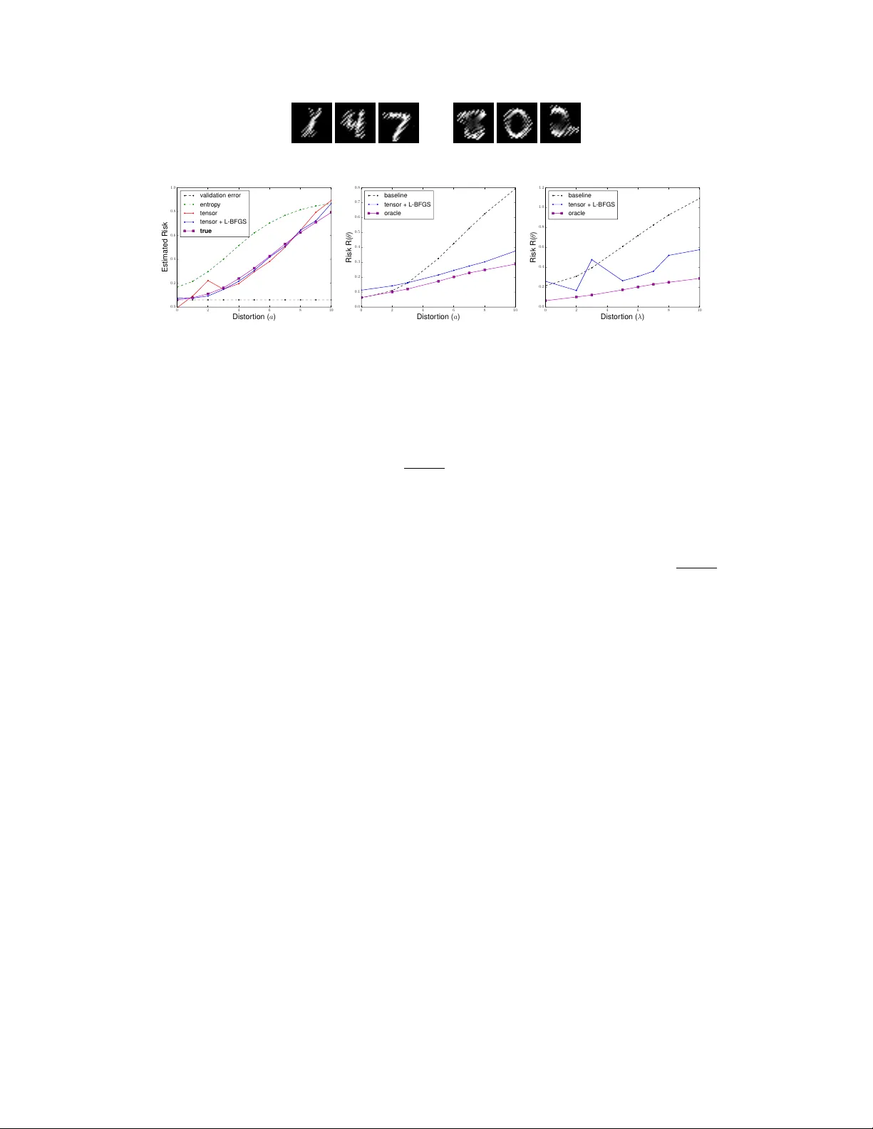
Unsupervised Risk Estimation Using Only Conditional Independence Structur e Jacob Steinhardt Computer Science Department Stanford Univ ersity jsteinhardt@cs.stanford.edu Per cy Liang Computer Science Department Stanford Univ ersity pliang@cs.stanford.edu Abstract W e show ho w to estimate a model’ s test error from unlabeled data, on distributions very different from the training distribution, while assuming only that certain conditional independencies are preserv ed between train and test. W e do not need to assume that the optimal predictor is the same between train and test, or that the true distribution lies in an y parametric family . W e can also ef ficiently dif ferentiate the error estimate to perform unsupervised discriminativ e learning. Our technical tool is the method of moments, which allows us to e xploit conditional independencies in the absence of a fully-specified model. Our framew ork encompasses a large family of losses including the log and e xponential loss, and extends to structured output settings such as hidden Markov models. 1 Introduction How can we assess the accuracy of a model when the test distribution is very different than the training distribution? T o address this question, we study the problem of unsupervised risk estimation ( Donmez et al. , 2010 )—that is, giv en a loss function L ( θ ; x, y ) and a fixed model θ , estimate the risk R ( θ ) def = E x,y ∼ p ∗ [ L ( θ ; x, y )] with respect to a test distribution p ∗ ( x, y ) , giv en access only to m unlabeled examples x (1: m ) ∼ p ∗ ( x ) . Unsupervised risk estimation lets us estimate model accuracy on a no vel input distrib ution, and is thus important for b uilding reliable machine learning systems. Beyond e v aluating a single model, it also provides a w ay of harnessing unlabeled data for learning: by minimizing the estimated risk over θ , we can perform unsupervised learning and domain adaptation. Unsupervised risk estimation is impossible without some assumptions on p ∗ , as otherwise p ∗ ( y | x ) — about which we ha ve no observable information—could be arbitrary . How satisfied we should be with an estimator depends on ho w strong its underlying assumptions are. In this paper , we present an approach which rests on surprisingly weak assumptions—that p ∗ satisfies certain conditional independencies, but not that it lies in an y parametric family or is close to the training distrib ution. T o giv e a fla vor for our results, suppose that y ∈ { 1 , . . . , k } and that the loss decomposes as a sum of three parts: L ( θ ; x, y ) = P 3 v =1 f v ( θ ; x v , y ) , where x 1 , x 2 , and x 3 are independent conditioned on y . In this case, we can estimate the risk to error  in p oly( k ) / 2 samples, independently of the dimension of x or θ ; the dependence on k is roughly cubic in practice. In Sections 2 and 3 we generalize this result to capture both the log and exponential losses, and e xtend beyond the multiclass case to allow y to be the hidden state of a hidden Markov model. Some intuition is provided in Figure 1 . At a fixed value of x , we can think of each f v as “predicting” that y = j if f v ( x v , j ) is low and f v ( x v , j 0 ) is high for j 0 6 = j . Since f 1 , f 2 , and f 3 all provide independent signals about y , their rate of agreement gi ves information about the model accurac y . If f 1 , f 2 , and f 3 all predict that y = 1 , then it is likely that the true y equals 1 and the loss is small. Con versely , if f 1 , f 2 , and f 3 all predict different values of y , then the loss is likely larger . This 1 2 3 4 1 2 3 4 1 2 3 4 y y y f 1 f 2 f 3 1 2 3 4 1 2 3 4 1 2 3 4 y y y f 1 f 2 f 3 Figure 1: T w o possible loss profiles at a giv en value of x . Left: if f 1 , f 2 , and f 3 are all minimized at the same value of y , that is likely to be the correct value and the total loss is likely to be small. Right: con versely , if f 1 , f 2 , and f 3 are small at differing v alues of y , then the loss is likely to be large. intuition is formalized by Dawid and Skene ( 1979 ) when the f v take values in a discrete set (e.g. when the f v measure the 0 / 1 -loss of independent classifiers); they model ( f 1 , f 2 , f 3 ) as a mixture of independent categorical variables, and use this to impute y as the label of the mixture component. Sev eral others ha ve e xtended this idea (e.g. Zhang et al. , 2014 ; Platanios , 2015 ; Jaf fe et al. , 2015 ), but continue to focus on the 0 / 1 loss (with a single exception that we discuss below). Why ha ve continuous losses such as the log loss been ignored, gi v en their utility for gradient-based learning? The issue is that while the 0 / 1 -loss only in v olves a discrete prediction in { 1 , . . . , k } (the predicted output), the log loss in volv es predictions in R k (the predicted probability distribution o ver outputs). The former can be fully modeled by a k -dimensional family , while the latter requires infinitely many parameters. W e could assume that the predictions are distributed according to some parametric family , but if that assumption is wrong then our risk estimates will be wrong as well. T o sidestep this issue, we make use of the method of moments ; while the method of moments has seen recent use in machine learning for fitting non-con ve x latent v ariable models (e.g. Anandkumar et al. , 2012 ), it has a much older history in the econometrics literature, where it has been used as a tool for making causal identifications under structural assumptions, e v en when an explicit form for the likelihood is not kno wn ( Anderson and Rubin , 1949 ; 1950 ; Sargan , 1958 ; 1959 ; Hansen , 1982 ; Powell , 1994 ; Hansen , 2014 ). It is upon this older literature that we draw conceptual inspiration, though our technical tools are more closely based on the newer machine learning approaches. The key insight is that certain moment equations–e.g., E [ f 1 f 2 | y ] = E [ f 1 | y ] E [ f 2 | y ] – can be deri ved from the assumed independencies; we then show ho w to estimate the risk while relying only on these moment conditions, and not on any parametric assumptions about the x v or f v . Moreover , these moment equations also hold for the gradient of f v , which enables efficient unsupervised learning. Our paper is structured as follows. In Section 2 , we present our basic framework, and state and prov e our main result on estimating the risk given f 1 , f 2 , and f 3 . In Section 3 , we extend our framework in sev eral directions, including to hidden Markov models. In Section 4 , we present a gradient-based learning algorithm and show that the sample comple xity needed for learning is d · p oly( k ) / 2 , where d is the dimension of θ . In Section 5 , we in vestigate ho w our method performs empirically . Related W ork. While the formal problem of unsupervised risk estimation w as only posed recently by Donmez et al. ( 2010 ), se veral older ideas from domain adaptation and semi-supervised learning are also rele vant. The covariate shift assumption assumes access to labeled samples from a base distribution p 0 ( x, y ) for which p ∗ ( y | x ) = p 0 ( y | x ) . If p ∗ ( x ) and p 0 ( x ) are close together , we can approximate p ∗ by p 0 via sample re-weighting ( Shimodaira , 2000 ; Quiñonero-Candela et al. , 2009 ). If p ∗ and p 0 are not close, another approach is to assume a well-specified discriminativ e model family Θ , such that p 0 ( y | x ) = p ∗ ( y | x ) = p θ ∗ ( y | x ) for some θ ∗ ∈ Θ ; then we need only heed finite-sample error in the estimation of θ ∗ ( Blitzer et al. , 2011 ; Li et al. , 2011 ). Both assumptions are somewhat stringent — re-weighting only allows small perturbations, and mis-specified models are common in practice. Indeed, many authors report that mis-specification can lead to se vere issues in semi-supervised settings ( Merialdo , 1994 ; Nigam et al. , 1998 ; Cozman and Cohen , 2006 ; Liang and Klein , 2008 ; Li and Zhou , 2015 ). As mentioned above, our approach is closer in spirit to that of Dawid and Skene ( 1979 ) and its extensions. Similarly to Zhang et al. ( 2014 ) and Jaf fe et al. ( 2015 ), we use the method of moments for estimating latent-variable models Ho we ver , those papers use it as a tool for parameter estimation in the face of non-con vexity , rather than as a way to sidestep model mis-specification. The insight that moments are robust to model mis-specification lets us extend beyond the simple discrete settings they consider in order to handle more comple x continuous and structured losses. Another approach to handling continuous losses is gi ven in the intriguing work of Balasubramanian et al. ( 2011 ), who sho w that the distrib ution of losses L | y is often close to Gaussian in practice, and use this to estimate 2 label: inputs: y x 1 x 2 x 3 y t − 2 y t − 1 y t y t +1 x t − 2 x t − 1 x t x t +1 y z x 1 x 2 x 3 Figure 2: Left: our basic 3 -view setup (Assumption 1 ). Center: Extension 1 , to hidden Markov models; the embedding of 3 views into the HMM is indicated in blue. Right: Extension 3 , to include a mediating variable z . the risk. A key dif ference from all of this prior work is that we are the first to perform gradient-based learning and the first to handle a structured loss (in our case, the log loss for hidden Markov models). 2 Framework and Estimation Algorithm W e will focus on multiclass classification; we assume an unknown true distribution p ∗ ( x, y ) ov er X × Y , where Y = { 1 , . . . , k } , and are given unlabeled samples x (1) , . . . , x ( m ) drawn i.i.d. from p ∗ ( x ) . Given parameters θ ∈ R d and a loss function L ( θ ; x, y ) , our goal is to estimate the risk of θ on p ∗ : R ( θ ) def = E x,y ∼ p ∗ [ L ( θ ; x, y )] . Throughout, we will make the 3-view assumption : Assumption 1 (3-vie w) . Under p ∗ , x can be split into x 1 , x 2 , x 3 , which are conditionally independent given y (see F igur e 2 ). Mor eover , the loss decomposes additively acr oss views: L ( θ ; x, y ) = A ( θ ; x ) − P 3 v =1 f v ( θ ; x v , y ) , for some functions A and f v . Note that if we hav e v > 3 views x 1 , . . . , x v , then we can always partition the views into blocks x 0 1 = x 1: b v / 3 c , x 0 2 = x b v / 3 c +1: b 2 v/ 3 c , x 0 3 = x b 2 v / 3 c +1: v . Assumption 1 then holds for x 0 1 , x 0 2 , x 0 3 . 1 In addition, it suffices for just the f v to be independent rather than the x v . W e will giv e some e xamples where Assumption 1 holds, then state and prov e our main result. W e start with logistic regression, which will be our primary focus later on: Example 1 (Logistic Regression) . Suppose that we hav e a log-linear model p θ ( y | x ) = exp  θ > ( φ 1 ( x 1 , y ) + φ 2 ( x 2 , y ) + φ 3 ( x 3 , y )) − A ( θ ; x )  , where x 1 , x 2 , and x 3 are independent conditioned on y . If our loss function is the log-loss L ( θ ; x, y ) = − log p θ ( y | x ) , then Assumption 1 holds with f v ( θ ; x v , y ) = θ > φ v ( x v , y ) , and A ( θ ; x ) equal to the partition function of p θ . W e next consider the hinge loss, for which Assumption 1 does not hold. Howe ver , it does hold for a modified hinge loss, where we apply the hinge separately to each view: Example 2 (Modified Hinge Loss) . Suppose that L ( θ ; x, y ) = P 3 v =1 (1 + max j 6 = y θ > φ v ( x v , j ) − θ > φ v ( x v , y )) + . In other words, L is the sum of 3 hinge losses, one for each view . Then Assumption 1 holds with A = 0 , and − f v equal to the hinge loss for view v . There is nothing special about the hinge loss; for instance, we could instead take a sum of 0 / 1 -losses. Our final example sho ws that linearity is not necessary for Assumption 1 to hold; the model can be arbitrarily non-linear in each view x v , as long as the predictions are combined additiv ely at the end: Example 3 (Neural Networks) . Suppose that for each vie w v we ha ve a neural netw ork whose output is a prediction v ector ( f v ( θ ; x v , j )) k j =1 . Suppose further that we add together the predictions f 1 + f 2 + f 3 , apply a soft-max, and e v aluate using the log loss; then L ( θ ; x, y ) = A ( θ ; x ) − P 3 v =1 f v ( θ ; x v , y ) , where A ( θ ; x ) is the log-normalization constant of the softmax, and hence L satisfies Assumption 1 . W ith these examples in hand, we are ready for our main result on recovering the risk R ( θ ) . The key is to recov er the conditional risk matrices M v ∈ R k × k , defined as ( M v ) ij = E [ f v ( θ ; x v , i ) | y = j ] . (1) 1 For v = 2 views, reco vering R is related to non-neg ativ e matrix f actorization ( Lee and Seung , 2001 ). Exact identification ends up being impossible, though obtaining upper bounds is likely possible. 3 In the case of the 0 / 1 -loss, the M v are confusion matrices; in general, ( M v ) ij measures ho w strongly we predict class i when the true class is j . If we could recover these matrices along with the marginal class probabilities π j def = p ∗ ( y = j ) , then estimating the risk would be straightforward; indeed, R ( θ ) = E [ A ( θ ; x )] − k X j =1 π j 3 X v =1 ( M v ) j,j , (2) where E [ A ( θ ; x )] can be estimated from unlabeled data alone. Cav eat: Class permutation. Suppose that at training time, we learn to predict whether an image con- tains the digit 0 or 1 . At test time, nothing changes except the definitions of 0 and 1 are rev ersed. It is clearly impossible to detect this from unlabeled data; mathematically , this manifests as M v only being recov erable up to column permutation. W e will end up computing the minimum risk ov er these permu- tations, which we call the optimistic risk and denote ˜ R ( θ ) def = min σ ∈ Sym( k ) E x,y ∼ p ∗ [ L ( θ ; x, σ ( y ))] . This equals the true risk as long as θ is at least aligned with the correct labels in the sense that E x [ L ( θ ; x, j ) | y = j ] ≤ E x [ L ( θ ; x, j 0 ) | y = j ] for j 0 6 = j . The optimal σ can then be computed from M v and π in O  k 3  time using maximum weight bipartite matching; see Section A for details. Our main result, Theorem 1 , says that we can recov er both M v and π up to permutation, with a number of samples that is polynomial in k ; in practice the dependence on k seems roughly cubic. Theorem 1. Suppose Assumption 1 holds. Then, for any , δ ∈ (0 , 1) , we can estimate M v and π up to column permutation, to err or  (in F r obenius and ∞ -norm respectively). Our algorithm r equir es m = p oly  k , π − 1 min , λ − 1 , τ  · log(2 /δ )  2 samples to succeed with pr obability 1 − δ , where π min def = k min j =1 p ∗ ( y = j ) , τ def = E  P v ,j f v ( θ ; x v , j ) 2  , and λ def = 3 min v =1 σ k ( M v ) , (3) and σ k denotes the k th singular value. Mor eover , the algorithm runs in time m · p oly( k ) . Note that estimates for M v and π imply an estimate for ˜ R via ( 2 ) . Importantly , the sample comple xity in Theorem 1 depends on the number of classes k , but not on the dimension d of θ . Moreov er , Theorem 1 holds e ven if p ∗ lies outside the model family θ , and ev en if the train and test distrib utions are very dif ferent (in fact, the result is totally agnostic to how the model θ was produced). The only requirement is that the 3 -view assumption holds for p ∗ . Let us interpret each term in ( 3 ) . First, τ tracks the variance of the loss, and we should expect the difficulty of estimating the risk to increase with this variance. The log(2 /δ )  2 term is typical and shows up e ven when estimating the parameter of a Bernoulli v ariable to accuracy  from m samples. The π − 1 min term appears because, if one of the classes is very rare, we need to wait a long time to observ e ev en a single sample from that class, and e ven longer to estimate the risk on that class accurately . Perhaps least intuitiv e is the λ − 1 term, which is large e.g. when two classes ha ve similar conditional risk vectors E [( f v ( θ ; x v , i )) k i =1 | y = j ] . T o see why this matters, consider an extreme where x 1 , x 2 , and x 3 are independent not only of each other but also of y . Then p ∗ ( y ) is completely unconstrained, and it is impossible to estimate R at all. Why does this not contradict Theorem 1 ? The answer is that in this case, all rows of M v are equal and hence λ = 0 , λ − 1 = ∞ , and we need infinitely many samples for Theorem 1 to hold; λ thus measures how close we are to this degenerate case. Proof of Theorem 1 . W e now outline a proof of Theorem 1 . Recall the goal is to estimate the conditional risk matrices M v , defined as ( M v ) ij = E [ f v ( θ ; x v , i ) | y = j ] ; from these we can recov er the risk itself using ( 2 ) . The key insight is that certain moments of p ∗ ( y | x ) can be e xpressed as polynomial functions of the matrices M v , and therefore we can solve for the M v ev en without explicitly estimating p ∗ . Our approach follows the technical machinery behind the spectral method of moments (e.g., Anandkumar et al. , 2012 ), which we explain belo w for completeness. Define the loss vector h v ( x v ) = ( f v ( θ ; x v , i )) k i =1 . The conditional independence of the x v means that E [ h 1 ( x 1 ) h 2 ( x 2 ) > | y ] = E [ h 1 ( x 1 ) | y ] E [ h 2 ( x 2 ) | y ] > , and similarly for higher-order conditional moments. There is thus low-rank structure in the moments of h , which we can exploit. More precisely , 4 Algorithm 1 Algorithm for estimating ˜ R ( θ ) from unlabeled data. 1: Input : unlabeled samples x (1) , . . . , x ( m ) ∼ p ∗ ( x ) . 2: Estimate the left-hand-side of each term in ( 4 ) using x (1: m ) . 3: Compute approximations ˆ M v and ˆ π v to M v and π using tensor decomposition. 4: Compute σ maximizing P k j =1 ˆ π σ ( j ) P 3 v =1 ( ˆ M v ) j,σ ( j ) using maximum bipartite matching. 5: Output : estimated 1 m P m i =1 A ( θ ; x ( i ) ) − P k j =1 ˆ π σ ( j ) P 3 v =1 ( ˆ M v ) j,σ ( j ) . by marginalizing o ver y , we obtain the following equations, where ⊗ denotes outer product: E [ h v ( x v )] = M v π , E [ h v ( x v ) h v 0 ( x v 0 ) > ] = M v diag( π ) M > v 0 for v 6 = v 0 , and E [ h 1 ( x 1 ) ⊗ h 2 ( x 2 ) ⊗ h 3 ( x 3 )] i 1 ,i 2 ,i 3 = k X j =1 π j · ( M 1 ) i 1 ,j ( M 2 ) i 2 ,j ( M 3 ) i 3 ,j ∀ i 1 , i 2 , i 3 . (4) The left-hand-side of each equation can be estimated from unlabeled data; we can then solve for M v and π using tensor decomposition ( Lathauwer , 2006 ; Comon et al. , 2009 ; Anandkumar et al. , 2012 ; 2013 ; Kulesho v et al. , 2015 ). In particular , we can recover M and π up to permutation: that is, we recov er ˆ M and ˆ π such that M i,j ≈ ˆ M i,σ ( j ) and π j ≈ ˆ π σ ( j ) for some permutation σ ∈ Sym( k ) . This then yields Theorem 1 ; see Section B for a full proof. Assumption 1 therefore yields a set of moment equations ( 4 ) that, when solved, let us estimate the risk without any labels y . T o summarize the procedure, we (i) approximate the left-hand-side of each term in ( 4 ) by sample a verages; (ii) use tensor decomposition to solve for π and M v ; (iii) use maximum matching to compute the permutation σ ; and (iv) use ( 2 ) to obtain ˜ R from π and M v . 3 Extensions Theorem 1 provides a basic building block which admits se veral e xtensions to more complex model structures. W e go over se veral cases belo w , omitting most proofs to av oid tedium. Extension 1 (Hidden Marko v Model) . Most importantly , the latent variable y need not belong to a small discrete set; we can handle structured output spaces such as a hidden Markov model as long as p ∗ matches the HMM structure. This is a substantial generalization of pre vious w ork on unsupervised risk estimation, which was restricted to multiclass classification. Suppose that p θ ( y 1: T | x 1: T ) ∝ Q T t =2 f θ ( y t − 1 , y t ) · Q T t =1 g θ ( y t , x t ) , with log-loss L ( θ ; x, y ) = − log p θ ( y 1: T | x 1: T ) . W e can exploit the decomposition − log p θ ( y 1: T | x 1: T ) = T X t =2 − log p θ ( y t − 1 , y t | x 1: T ) | {z } def = ` t − T X t =1 − log p θ ( y t | x 1: T ) | {z } def = ` 0 t . (5) Assuming that p ∗ is Markovian with respect to y , each of the losses ` t , ` 0 t satisfies Assumption 1 (see Figure 2 ; for ` t , the views are x 1: t − 2 , x t − 1: t , x t +1: T , and for ` 0 t they are x 1: t − 1 , x t , x t +1: T ). W e use Theorem 1 to estimate each E [ ` t ] , E [ ` 0 t ] individually , and thus also the full risk E [ L ] . (Note that we actually estimate the risk for y 2: T − 1 | x 1: T due to the 3 -view assumption f ailing at the boundaries.) In general, the idea in ( 5 ) applies to any structured output problem that is a sum of local 3 -view structures. It would be interesting to extend our results to other structures such as more general graphical models ( Chaganty and Liang , 2014 ) and parse trees ( Hsu et al. , 2012 ). Extension 2 (Exponential Loss) . W e can also relax the additivity condition L = A − f 1 − f 2 − f 3 . For instance, suppose L ( θ ; x, y ) = exp( − θ > P 3 v =1 φ v ( x v , y )) is the exponential loss. W e can use Theorem 1 to estimate the matrices M v corresponding to f v ( θ ; x v , y ) = exp( − θ > φ v ( x v , y )) . Then R ( θ ) = E " 3 Y v =1 f v ( θ ; x v , y ) # = X j π j 3 Y v =1 E [ f v ( θ ; x v , j ) | y = j ] (6) by conditional independence. Therefore, the risk can be estimated as P j π j Q 3 v =1 ( M v ) j,j . More generally , it suffices to hav e L ( θ ; x, y ) = A ( θ ; x ) + P n i =1 Q 3 v =1 f v i ( θ ; x v , y ) for some functions f v i . 5 Extension 3 (Mediating V ariable) . Assuming that x 1:3 are independent conditioned only on y may not be realistic; there might be multiple subclasses of a label (e.g., multiple ways to write the digit 4 ) which w ould induce systematic correlations across views. T o address this, we show that independence need only hold conditioned on a mediating variable z , rather than on the label y itself. Let z be a refinement of y (in the sense that z → y is deterministic) which takes on k 0 values, and suppose that the views x 1 , x 2 , x 3 are independent conditioned on z , as in Figure 2 . Then we can estimate the risk as long as we can e xtend the loss v ector h v = ( f v ) k i =1 to a function h 0 v : X v → R k 0 , such that h 0 v ( x v ) i = f v ( x v , i ) and the matrix ( M 0 v ) ij = E [ h 0 v ( x v ) i | z = j ] has full rank. The reason is that we can reco ver the matrices M 0 v , and then, letting r be the map from z to y , we can e xpress the risk as R ( θ ) = E [ A ( θ ; x )] + P k 0 j =1 p ∗ ( z = j ) P 3 v =1 ( M 0 v ) r ( j ) ,j . Summary . Our frame work applies to the log loss and exponential loss; to hidden Markov models; and to cases where there are latent variables mediating the independence structure. 4 From Estimation to Learning W e no w turn our attention to unsupervised learning, i.e., minimizing R ( θ ) ov er θ ∈ R d . Unsupervised learning is impossible without some additional information, since e v en if we could learn the k classes, we wouldn’t kno w which class had which label. Thus we assume that we have a small amount of information to break this symmetry , in the form of a seed model θ 0 : Assumption 2 (Seed Model) . W e have access to a “seed model” θ 0 such that ˜ R ( θ 0 ) = R ( θ 0 ) . Assumption 2 merely asks for θ 0 to be aligned with the true labels on average. W e can obtain θ 0 from a small amount of labeled data (semi-supervised learning) or by training in a nearby domain (domain adaptation). W e define gap( θ 0 ) to be the difference between R ( θ 0 ) and the next smallest permutation of the classes, which will affect the dif ficulty of learning. For simplicity we will focus on the case of logistic regression, and show how to learn giv en only Assumptions 1 and 2 . Howe ver , our algorithm e xtends to general losses, as we sho w in Section E . Learning from moments. Note that for logistic re gression (Examples 1 ), the unobserved components of L ( θ ; x, y ) are linear in the sense that f v ( θ ; x v , y ) = θ > φ v ( x v , y ) for some φ v . W e therefore have R ( θ ) = E [ A ( θ ; x )] − θ > ¯ φ, where ¯ φ def = 3 X v =1 E [ φ v ( x v , y )] . (7) From ( 7 ) , we see that it suf fices to estimate ¯ φ , after which all terms on the right-hand-side of ( 7 ) are known. Giv en an approximation ˆ φ to ¯ φ (we will show ho w to obtain ˆ φ below), we can learn a near-optimal θ by solving the following con v ex optimization problem: ˆ θ = arg min k θ k 2 ≤ ρ E [ A ( θ ; x )] − θ > ˆ φ. (8) In practice we would need to approximate E [ A ( θ ; x )] by samples, b ut we ignore this for simplicity (it only contributes lo wer -order terms to the error). The ` 2 -constraint on θ imparts robustness to errors in ¯ φ . In particular (see Section C for a proof): Lemma 1. Suppose k ˆ φ − ¯ φ k 2 ≤  . Then the output ˆ θ fr om ( 8 ) satisfies R ( ˆ θ ) ≤ min k θ k 2 ≤ ρ R ( θ ) + 2 ρ . Assuming that the optimal parameter θ ∗ has ` 2 -norm at most ρ , Lemma 1 guarantees that R ( ˆ θ ) ≤ R ( θ ∗ ) + 2 ρ . W e will see below that computing ˆ φ requires d · p oly  k , π − 1 min , λ − 1 , τ  / 2 samples. Computing ˆ φ . Estimating ¯ φ can be done in a manner similar to estimating R ( θ ) itself. In addition to the conditional risk matrix M v ∈ R k × k , we compute the conditional moment matrix G v ∈ R dk × k defined by ( G v ) i + kr,j def = E [ φ v ( θ ; x v , i ) r | y = j ] . W e then have ¯ φ r = P k j =1 π j P 3 v =1 ( G v ) j + k r,j . W e can solve for G 1 , G 2 , and G 3 using the same tensor algorithm as in Theorem 1 . Some care is needed to avoid explicitly forming the ( k d ) × ( k d ) × ( k d ) tensor that would result from the third term in ( 4 ) , as this would require O  k 3 d 3  memory and is thus intractable for ev en moderate values of d . W e take a standard approach based on random projections ( Halko et al. , 2011 ) and described in 6 Figure 3: A few sample train images (left) and test images (right) from the modified MNIST data set. 0 2 4 6 8 10 Distor tion ( a ) 0 . 0 0 . 2 0 . 4 0 . 6 0 . 8 1 . 0 Estimated Risk v alidation error entrop y tensor tensor + L-BFGS true (a) 0 2 4 6 8 10 Distor tion ( a ) 0 . 0 0 . 1 0 . 2 0 . 3 0 . 4 0 . 5 0 . 6 0 . 7 0 . 8 Risk R( θ ) baseline tensor + L-BFGS or acle (b) 0 2 4 6 8 10 Distor tion ( λ ) 0 . 0 0 . 2 0 . 4 0 . 6 0 . 8 1 . 0 1 . 2 Risk R( θ ) baseline tensor + L-BFGS or acle (c) Figure 4: Results on the modified MNIST data set. (a) Risk estimation for varying degrees of distortion a . (b) Domain adaptation with 10 , 000 training and 10 , 000 test examples. (c) Domain adaptation with 300 training and 10 , 000 test e xamples. Section 6.1.2 of Anandkumar et al. ( 2013 ). W e refer the reader to the aforementioned references for details, and cite only the final sample complexity and runtime (see Section D for a proof sketch): Theorem 2. Suppose that Assumption 1 holds and that θ 0 ∈ Θ 0 . Let δ < 1 and  < min(1 , gap( θ 0 )) . Then, given m = p oly  k , π − 1 min , λ − 1 , τ  · log(2 /δ )  2 samples, where λ and τ ar e as defined in ( 3 ) , with pr obability 1 − δ we can reco ver M v and π to err or  , and G v to err or ( B /τ )  , wher e B 2 = E [ P i,v k φ v ( x v , i ) k 2 2 ] measur es the ` 2 -norm of the features. The algorithm runs in time O ( d ( m + p oly ( k ))) , and the err ors ar e in F r obenius norm for M and G , and ∞ -norm for π . Interpr etation. Whereas before we estimated M v to error  , no w we estimate G v (and hence ¯ φ ) to error ( B /τ )  . T o achieve error  in estimating G v requires ( B /τ ) 2 · p oly  k , π − 1 min , λ − 1 , τ  log(2 /δ )  2 samples, which is ( B /τ ) 2 times as lar ge as in Theorem 1 . The quantity ( B /τ ) 2 typically gro ws as O ( d ) , and so the sample complexity needed to estimate ¯ φ is typically d times larger than the sample complexity needed to estimate R . This matches the behavior of the supervised case where we need d times as many samples for learning as compared to (supervised) risk estimation of a fix ed model. Summary . W e ha ve shown how to perform unsupervised logistic regression, given only a seed model θ 0 . This enables unsupervised learning under surprisingly weak assumptions (only the multi-view and seed model assumptions) ev en for mis-specified models and zero train-test overlap, and without assuming cov ariate shift. See Section E for learning under more general losses. 5 Experiments T o better understand the behavior of our algorithms, we perform experiments on a version of the MNIST data set that is modified to ensure that the 3 -view assumption holds. T o create an image, we sample a class in { 0 , . . . , 9 } , then sample 3 images at random from that class, letting ev ery third pixel come from the respecti ve image. This guarantees that there will be 3 conditionally independent views. T o explore train-test variation, we dim pixel p in the image by exp ( a ( k p − p 0 k 2 − 0 . 4)) , where p 0 is the image center and the distance is normalized to hav e maximum value 1 . W e show example images for a = 0 (train) and a = 5 (a possible test distrib ution) in Figure 3 . Risk estimation. W e use unsupervised risk estimation (Theorem 1 ) to estimate the risk of a model trained on a = 0 and tested on v arious values of a ∈ [0 , 10] . W e trained the model with AdaGrad ( Duchi et al. , 2010 ) on 10 , 000 training examples, and used 10 , 000 test examples to estimate the risk. T o solve for π and M in ( 4 ) , we first use the tensor power method implemented by Chaganty and Liang ( 2013 ) to initialize, and then locally minimize a weighted ` 2 -norm of the moment errors with L-BFGS. For comparison, we compute the v alidation error for a = 0 (i.e., assume train = test), as well as the predicti ve entropy P j − p θ ( j | x ) log p θ ( j | x ) on the test set (i.e., assume the predictions are well-calibrated). The results are shown in Figure 4a ; both the tensor method in isolation and tensor + L-BFGS estimate the risk accurately , with the latter performing slightly better . 7 Domain adaptation. W e next e v aluate our learning algorithm. For θ 0 we used the trained model at a = 0 , and constrained k θ k 2 ≤ 10 in ( 8 ) . The results are sho wn in Figure 4b . For small values of a , our algorithm performs worse than the baseline of directly using θ 0 . Howe ver , our algorithm is far more rob ust as a increases, and tracks the performance of an oracle that was trained on the same distribution as the test e xamples. Semi-supervised learning. Because we only need to pro vide our algorithm with a seed model, we can perform semi-supervised domain adaptation — train a model from a small amount of labeled data at a = 0 , then use unlabeled data to learn a better model on a new distribution. Concretely , we obtained θ 0 from only 300 labeled examples. T ensor decomposition sometimes led to bad initializations in this regime, in which case we obtained a different θ 0 by training with a smaller step size. The results are shown in Figure 4c . Our algorithm generally performs well, but has higher variability than before, seemingly due to higher condition number of the matrices M v . Summary . Our experiments sho w that giv en 3 views, we can estimate the risk and perform domain adaptation, ev en from a small amount of labeled data. 6 Discussion W e have presented a method for estimating the risk from unlabeled data, which relies only on conditional independence structure and hence makes no parametric assumptions about the true distribution. Our approach applies to a large family of losses and extends be yond classification tasks to hidden Markov models. W e can also perform unsupervised learning giv en only a seed model that can distinguish between classes in expectation; the seed model can be trained on a related domain, on a small amount of labeled data, or an y combination of the two, and thus pro vides a pleasingly general formulation highlighting the similarities between domain adaptation and semi-supervised learning. Previous approaches to domain adaptation and semi-supervised learning hav e also exploited multi- view structure. Giv en two vie ws, Blitzer et al. ( 2011 ) perform domain adaptation with zero source/target ov erlap (covariate shift is still assumed). T wo-vie w approaches (e.g. co-training and CCA) are also used in semi-supervised learning ( Blum and Mitchell , 1998 ; Ando and Zhang , 2007 ; Kakade and Foster , 2007 ; Balcan and Blum , 2010 ). These methods all assume some form of low noise or lo w regret, as do, e.g., transducti ve SVMs ( Joachims , 1999 ). By focusing on the central problem of risk estimation, our work connects multi-view learning approaches for domain adaptation and semi-supervised learning, and remov es covariate shift and low-noise/lo w-regret assumptions (though we make stronger independence assumptions, and specialize to discrete prediction tasks). In addition to reliability and unsupervised learning, our work is motiv ated by the desire to build machine learning system with contracts , a challenge recently posed by Bottou ( 2015 ); the goal is for machine learning systems to satisfy a well-defined input-output contract in analogy with softw are systems ( Sculley et al. , 2015 ). Theorem 1 provides the contract that under the 3 -view assumption the test error is close to our estimate of the test error; this contrasts with the typical weak contract that if train and test are similar , then the test error is close to the training error . One other interesting contract is giv en by Shafer and V o vk ( 2008 ), who provide prediction r e gions that contain the true prediction with probability 1 −  in the online setting, even in the presence of model mis-specification. The most restrictiv e part of our framework is the three-vie w assumption, which is inappropriate if the views are not completely independent or if the data hav e structure that is not captured in terms of multiple views. Since Balasubramanian et al. ( 2011 ) obtain results under Gaussianity (which would be implied by many some what dependent views), we are optimistic that unsupervised risk estimation is possible for a wider family of structures. Along these lines, we end with the following questions: Open question. In the 3 -view setting, suppose the views are not completely independent. Is it still possible to estimate the risk? How does the degree of dependence af fect the number of views needed? Open question. Giv en only two independent views, can one obtain an upper bound on the risk R ( θ ) ? The results of this paper have caused us to adopt the following perspective: T o handle unlabeled data, we should make generative structural assumptions, but still optimize discriminative model performance. This hybrid approach allows us to satisfy the traditional machine learning goal of predictiv e accurac y , while handling lack of supervision and under-specification in a principled way . Perhaps, then, what is needed for learning is to understand the structur e of a domain. 8 References A. Anandkumar, D. Hsu, and S. M. Kakade. A method of moments for mixture models and hidden Markov models. In Confer ence on Learning Theory (COLT) , 2012. A. Anandkumar , R. Ge, D. Hsu, S. M. Kakade, and M. T elgarsk y . T ensor decompositions for learning latent variable models. arXiv , 2013. T . W . Anderson and H. Rubin. Estimation of the parameters of a single equation in a complete system of stochastic equations. The Annals of Mathematical Statistics , pages 46–63, 1949. T . W . Anderson and H. Rubin. The asymptotic properties of estimates of the parameters of a single equation in a complete system of stochastic equations. The Annals of Mathematical Statistics , pages 570–582, 1950. R. K. Ando and T . Zhang. T w o-view feature generation model for semi-supervised learning. In Conference on Learning Theory (COLT) , pages 25–32, 2007. K. Balasubramanian, P . Donmez, and G. Lebanon. Unsupervised supervised learning II: Margin-based classifica- tion without labels. Journal of Mac hine Learning Resear ch (JMLR) , 12:3119–3145, 2011. M. Balcan and A. Blum. A discriminativ e model for semi-supervised learning. Journal of the ACM (J A CM) , 57 (3), 2010. J. Blitzer , S. Kakade, and D. P . Foster . Domain adaptation with coupled subspaces. In Artificial Intelligence and Statistics (AIST A TS) , pages 173–181, 2011. A. Blum and T . Mitchell. Combining labeled and unlabeled data with co-training. In Conference on Learning Theory (COLT) , 1998. L. Bottou. T w o high stakes challenges in machine learning. In vited talk at the 32nd International Conference on Machine Learning, 2015. A. Chaganty and P . Liang. Spectral experts for estimating mixtures of linear regressions. In International Confer ence on Machine Learning (ICML) , 2013. A. Chaganty and P . Liang. Estimating latent-variable graphical models using moments and likelihoods. In International Confer ence on Machine Learning (ICML) , 2014. P . Comon, X. Luciani, and A. L. D. Almeida. T ensor decompositions, alternating least squares and other tales. Journal of Chemometrics , 23(7):393–405, 2009. F . Cozman and I. Cohen. Risks of semi-supervised learning: How unlabeled data can degrade performance of generativ e classifiers. In Semi-Supervised Learning . 2006. A. P . Dawid and A. M. Skene. Maximum likelihood estimation of observer error -rates using the EM algorithm. Applied Statistics , 1:20–28, 1979. P . Donmez, G. Lebanon, and K. Balasubramanian. Unsupervised supervised learning I: Estimating classification and regression errors without labels. Journal of Machine Learning Resear c h (JMLR) , 11:1323–1351, 2010. J. Duchi, E. Hazan, and Y . Singer . Adaptiv e subgradient methods for online learning and stochastic optimization. In Confer ence on Learning Theory (COLT) , 2010. J. Edmonds and R. M. Karp. Theoretical improvements in algorithmic ef ficiency for netw ork flo w problems. Journal of the A CM (J A CM) , 19(2):248–264, 1972. N. Halko, P .-G. Martinsson, and J. Tropp. Finding structure with randomness: Probabilistic algorithms for constructing approximate matrix decompositions. SIAM Review , 53:217–288, 2011. L. P . Hansen. Large sample properties of generalized method of moments estimators. Econometrica: Journal of the Econometric Society , 50:1029–1054, 1982. L. P . Hansen. Uncertainty outside and inside economic models. Journal of P olitical Economy , 122(5):945–987, 2014. D. Hsu, S. M. Kakade, and P . Liang. Identifiability and unmixing of latent parse trees. In Advances in Neural Information Pr ocessing Systems (NIPS) , 2012. A. Jaffe, B. Nadler, and Y . Kluger. Estimating the accuracies of multiple classifiers without labeled data. In Artificial Intelligence and Statistics (AIST A TS) , pages 407–415, 2015. 9 T . Joachims. Transducti v e inference for text classification using support vector machines. In International Confer ence on Machine Learning (ICML) , 1999. S. M. Kakade and D. P . Foster . Multi-view regression via canonical correlation analysis. In Conference on Learning Theory (COLT) , pages 82–96, 2007. V . Kuleshov , A. Chaganty , and P . Liang. T ensor f actorization via matrix factorization. In Artificial Intelligence and Statistics (AIST A TS) , 2015. L. D. Lathauwer . A link between the canonical decomposition in multilinear algebra and simultaneous matrix diagonalization. SIAM Journal of Matrix Analysis and Applications , 28(3):642–666, 2006. D. D. Lee and S. H. Seung. Algorithms for non-ne gati ve matrix factorization. In Advances in Neur al Information Pr ocessing Systems (NIPS) , pages 556–562, 2001. L. Li, M. L. Littman, T . J. W alsh, and A. L. Strehl. Knows what it knows: a framework for self-aw are learning. Machine learning , 82(3):399–443, 2011. Y . Li and Z. Zhou. T owards making unlabeled data nev er hurt. IEEE T ransactions on P attern Analysis and Machine Intelligence , 37(1):175–188, 2015. P . Liang and D. Klein. Analyzing the errors of unsupervised learning. In Human Language T echnology and Association for Computational Linguistics (HLT/A CL) , 2008. B. Merialdo. T agging English text with a probabilistic model. Computational Linguistics , 20:155–171, 1994. K. Nigam, A. McCallum, S. Thrun, and T . Mitchell. Learning to classify text from labeled and unlabeled documents. In Association for the Advancement of Artificial Intelligence (AAAI) , 1998. E. A. Platanios. Estimating accuracy from unlabeled data. Master’ s thesis, Carne gie Mellon Univ ersity , 2015. J. L. Powell. Estimation of semiparametric models. In Handbook of Econometrics , volume 4, pages 2443–2521. 1994. J. Quiñonero-Candela, M. Sugiyama, A. Schwaighofer , and N. D. Lawrence. Dataset shift in machine learning . The MIT Press, 2009. J. D. Sargan. The estimation of economic relationships using instrumental variables. Econometrica , pages 393–415, 1958. J. D. Sargan. The estimation of relationships with autocorrelated residuals by the use of instrumental variables. Journal of the Royal Statistical Society: Series B (Statistical Methodology) , pages 91–105, 1959. D. Sculley , G. Holt, D. Golovin, E. Davydov , T . Phillips, D. Ebner, V . Chaudhary , M. Y oung, J. Crespo, and D. Dennison. Hidden technical debt in machine learning systems. In Advances in Neural Information Pr ocessing Systems (NIPS) , pages 2494–2502, 2015. G. Shafer and V . V ovk. A tutorial on conformal prediction. Journal of Machine Learning Resear c h (JMLR) , 9: 371–421, 2008. H. Shimodaira. Improving predicti ve inference under co v ariate shift by weighting the log-likelihood function. Journal of Statistical Planning and Infer ence , 90:227–244, 2000. J. Steinhardt, G. V aliant, and S. W ager . Memory , communication, and statistical queries. Electronic Colloquium on Computational Complexity (ECCC) , 22, 2015. N. T omiza wa. On some techniques useful for solution of transportation network problems. Networks , 1(2): 173–194, 1971. Y . Zhang, X. Chen, D. Zhou, and M. I. Jordan. Spectral methods meet EM: A provably optimal algorithm for crowdsourcing. arXiv , 2014. 10 A Details of Computing ˜ R from M and π In this section we show ho w , gi ven M , and π , we can efficiently compute ˜ R ( θ ) = E [ A ( θ ; x )] − max σ ∈ Sym( k ) k X j =1 π σ ( j ) 3 X v =1 ( M v ) j,σ ( j ) . (9) The only bottleneck is the maximum over σ ∈ Sym( k ) , which would naïvely require considering k ! possibilities. Howe ver , we can instead cast this as a form of maximum matching. In particular, form the k × k matrix X i,j = π i 3 X v =1 ( M v ) j,i . (10) Then we are looking for the permutation σ such that P k j =1 X σ ( j ) ,j is maximized. If we consider each X i,j to be the weight of edge ( i, j ) in a complete bipartite graph, then this is equiv alent to asking for a matching of i to j with maximum weight, hence we can maximize over σ using any maximum-weight matching algorithm such as the Hungarian algorithm, which runs in O  k 3  time ( T omizawa , 1971 ; Edmonds and Karp , 1972 ). B Proof of Theorem 1 Preliminary reductions. Our goal is to estimate M and π to error  (with probability of failure 1 − δ ) in p oly  k , π − 1 min , λ − 1 , τ  · log(1 /δ )  2 samples. Note that if we can estimate M and π to error  with any fix ed probability of success 1 − δ 0 ≥ 3 4 , then we can amplify the probability of success to 1 − δ at the cost of O (log(1 /δ )) times as many samples (the idea is to make sev eral independent estimates, then thro w out any estimate that is more than 2  away from at least half of the others; all the remaining estimates will then be within distance 3  of the truth with high probability). Estimating M . Estimating π and M is mostly an ex ercise in interpreting Theorem 7 of Anandkumar et al. ( 2012 ), which we recall below , modifying the statement slightly to fit our language. Here κ denotes condition number (which is the ratio of σ 1 ( M ) to σ k ( M ) , since all matrices in question ha v e k columns). Theorem 3 ( Anandkumar et al. ( 2012 )) . Let P v ,v 0 def = E [ h v ( x ) ⊗ h v 0 ( x )] , and P 1 , 2 , 3 def = E [ h 1 ( x ) ⊗ h 2 ( x ) ⊗ h 3 ( x )] . Also let ˆ P v ,v 0 and ˆ P 1 , 2 , 3 be sample estimates of P v ,v 0 , P 1 , 2 , 3 that ar e (for technical con venience) estimated fr om independent samples of size m . Let k T k F denote the ` 2 -norm of T after unr olling T to a vector . Suppose that: • P  k ˆ P v ,v 0 − P v ,v 0 k 2 ≤ C v ,v 0 q log(1 /δ ) m  ≥ 1 − δ for { v , v 0 } ∈ {{ 1 , 2 } , { 1 , 3 }} , and • P  k ˆ P 1 , 2 , 3 − P 1 , 2 , 3 k F ≤ C 1 , 2 , 3 q log(1 /δ ) m  ≥ 1 − δ . Then, ther e e xists constants C , m 0 , δ 0 such that the following holds: if m ≥ m 0 and δ ≤ δ 0 and r log( k /δ ) m ≤ C · min j 6 = j 0 k ( M > 3 ) j − ( M > 3 ) j 0 k 2 · σ k ( P 1 , 2 ) C 1 , 2 , 3 · k 5 · κ ( M 1 ) 4 · δ log( k /δ ) · , r log(1 /δ ) m ≤ C · min  min j 6 = j 0 k ( M > 3 ) j − ( M > 3 ) j 0 k 2 · σ k ( P 1 , 2 ) 2 C 1 , 2 · k P 1 , 2 , 3 k F · k 5 · κ ( M 1 ) 4 · δ log( k /δ ) , σ k ( P 1 , 3 ) C 1 , 3  · , then with pr obability at least 1 − 5 δ , we can output ˆ M 3 with the following guarantee: ther e exists a permutation σ ∈ Sym( k ) suc h that for all j ∈ { 1 , . . . , k } , k ( M > 3 ) j − ( ˆ M > 3 ) σ ( j ) k 2 ≤ max j 0 k ( M > 3 ) j 0 k 2 · . (11) 11 By symmetry , we can use Theorem 3 to recover each of the matrices M v , v = 1 , 2 , 3 , up to permutation of the columns. Furthermore, Anandkumar et al. ( 2012 ) show in Appendix B.4 of their paper ho w to match up the columns of the different M v , so that only a single unknown permutation is applied to each of the M v simultaneously . W e will set δ = 1 / 180 , which yields an o verall probability of success of 11 / 12 for this part of the proof. W e now analyze the rate of con ver gence implied by Theorem 3 . Note that we can take C 1 , 2 , 3 = O  p E [ k h 1 k 2 2 k h 2 k 2 2 k h 3 k 2 2 ]  , and similarly C v ,v 0 = O  p E [ k h v k 2 2 k h v 0 k 2 2 ]  . Then, since we only care about polynomial factors, it is enough to note that we can estimate the M v to error  giv en Z/ 2 samples, where Z is polynomial in the following quantities: 1. k , 2. max 3 v =1 κ ( M v ) , where κ denotes condition number, 3. √ E [ k h 1 k 2 2 k h 2 k 2 2 k h 3 k 2 2 ] ( min j,j 0 k ( M > v ) j − ( M > v ) j 0 k 2 ) · σ k ( P v 0 ,v 00 ) , where ( v , v 0 , v 00 ) is a permutation of (1 , 2 , 3) , 4. k P 1 , 2 , 3 k 2 ( min j,j 0 k ( M > v ) j − ( M > v ) j 0 k 2 ) · σ k ( P v 0 ,v 00 ) , where ( v , v 0 , v 00 ) is as before, and 5. √ E [ k h v k 2 2 k h v 0 k 2 2 ] σ k ( P v,v 0 ) . 6. max j,v k ( M > v ) j k 2 . It suffices to sho w that each of these quantities are polynomial in k , π − 1 min , τ , and λ − 1 . (1) k is trivially polynomial in itself. (2) Note that κ ( M v ) ≤ σ 1 ( M v ) /λ ≤ k M v k F /λ . Furthermore, k M v k 2 F = P j k E [ h v | j ] k 2 2 ≤ P j E [ k h v k 2 2 | j ] ≤ k τ 2 . In all, κ ( M v ) ≤ √ k τ /λ , which is polynomial in k and τ /λ . (3) W e first note that min j 6 = j 0 k ( M > v ) j − ( M > v ) j 0 k 2 = √ 2 min j 6 = j 0 k M > v ( e j − e j 0 ) k 2 / k e j − e j 0 k 2 ≥ σ k ( M v ) . Also, σ k ( P v 0 ,v 00 ) = σ k ( M v 0 diag( π ) M v 00 ) ≥ σ k ( M v 0 ) π min σ k ( M v 00 ) . W e can thus upper- bound the quantity in (3.) by p E [ k h 1 k 2 2 k h 2 k 2 2 k h 3 k 2 2 ] √ 2 π min σ k ( M 1 ) σ k ( M 2 ) σ k ( M 3 ) ≤ τ 3 √ 2 π min λ 3 , which is polynomial in π − 1 min , τ /λ . (4) W e can perform the same calculations as in (3), but now we ha ve to bound k P 1 , 2 , 3 k 2 . Ho wev er , it is easy to see that k P 1 , 2 , 3 k 2 = q k E [ h 1 ⊗ h 2 ⊗ h 3 ] k 2 2 ≤ q E [ k h 1 ⊗ h 2 ⊗ h 3 k 2 2 ] = q E [ k h 1 k 2 2 k h 2 k 2 2 k h 3 k 2 2 ] = v u u t k X j =1 π j 3 Y v =1 E [ k h v k 2 2 | y = j ] ≤ τ 3 , which yields the same upper bound as in (3). (5) W e can again perform the same calculations as in (3), where we no w only hav e to deal with a subset of the variables, thus obtaining a bound of τ 2 π min λ 2 . (6) W e hav e k ( M > v ) j k 2 ≤ p E [ k h v k 2 2 | y = j ] ≤ τ . In sum, we ha ve sho wn that with probability 11 12 we can estimate each M v to column-wise ` 2 error  using p oly  k , π − 1 min , λ − 1 , τ  / 2 samples; since there are only k columns, we can make the total 12 (Frobenius) error be at most  while still using p oly  k , π − 1 min , λ − 1 , τ  / 2 samples. It now remains to estimate π . Estimating π . This part of the argument follows Appendix B.5 of Anandkumar et al. ( 2012 ). Noting that π = M − 1 1 E [ h 1 ] , we can estimate π as ˆ π = ˆ M 1 − 1 ˆ E [ h 1 ] , where ˆ E denotes the empirical expectation. Hence, we hav e k π − ˆ π k ∞ ≤    ( ˆ M 1 − 1 − M − 1 1 ) E [ h 1 ] + M − 1 1 ( ˆ E [ h 1 ] − E [ h 1 ]) + ( ˆ M 1 − 1 − M − 1 1 )( ˆ E [ h 1 ] − E [ h 1 ])    ∞ ≤ k ˆ M 1 − 1 − M − 1 1 k F | {z } ( i ) k E [ h 1 ] k 2 | {z } ( ii ) + k M − 1 1 k F | {z } ( iii ) k ˆ E [ h 1 ] − E [ h 1 ] k 2 | {z } ( iv ) + k ˆ M 1 − 1 − M − 1 1 k F | {z } ( i ) k ˆ E [ h 1 ] − E [ h 1 ] k 2 | {z } ( iv ) . W e will bound each of these factors in turn: (i) k ˆ M 1 − 1 − M − 1 1 k F : let E 1 = ˆ M 1 − M 1 , which by the previous part satisfies k E 1 k F ≤ √ k max j k ( ˆ M > 1 ) j − ( M > 1 ) j k 2 = p oly  k , π − 1 min , λ − 1 , τ  / √ m . Therefore: k ˆ M 1 − 1 − M − 1 1 k F ≤ k ( M 1 + E 1 ) − 1 − M − 1 1 k F = k M − 1 1 ( I + E 1 M − 1 1 ) − 1 − M − 1 1 k F ≤ k M − 1 1 k F k ( I + E 1 M − 1 1 ) − 1 − I k F ≤ k λ − 1 σ 1  I + E 1 M − 1 1 ) − 1 − I  ≤ k λ − 1 σ 1 ( E 1 M − 1 1 ) 1 − σ 1 ( E 1 M − 1 1 ) ≤ k λ − 2 k E 1 k F 1 − λ − 1 k E 1 k F ≤ p oly  k , π − 1 min , λ − 1 , τ  1 − p oly  k , π − 1 min , λ − 1 , τ  / √ m · 1 √ m . W e can assume that m ≥ p oly  k , π − 1 min , λ − 1 , τ  without loss of generality (since otherwise we can tri vially obtain the desired bound on k π − ˆ π k ∞ by simply guessing the uniform distribution), in which case the abo ve quantity is poly  k , π − 1 min , λ − 1 , τ  · 1 √ m . (ii) k E [ h 1 ] k 2 : we have k E [ h 1 ] k 2 ≤ p E [ k h 1 k 2 2 ] ≤ τ . (iii) k M − 1 1 k F : since k X k F ≤ √ k σ 1 ( F ) , we hav e k M − 1 1 k F ≤ √ k λ − 1 . (iv) k ˆ E [ h 1 ] − E [ h 1 ] k 2 : with any fixed probability (say 11 / 12 ), this term is O  q E [ k h 1 k 2 2 ] m  = O  τ √ m  . In sum, with probability at least 11 12 all of the terms are p oly  k , π − 1 min , λ − 1 , τ  , and at least one factor in each term has a 1 √ m decay . Therefore, we have k π − ˆ π k ∞ ≤ p oly  k , π − 1 min , λ − 1 , τ  · q 1 m . Since we hav e shown that we can estimate each of M and π indivi dually with probability 11 12 , we can estimate them jointly 5 6 > 3 4 , thus completing the proof. 13 C Proof of Lemma 1 Let B ( ρ ) = { θ | k θ k 2 ≤ ρ } . First note that | θ > ( ˆ φ − ¯ φ ) | ≤ k θ k 2 k ˆ φ − ¯ φ k 2 ≤ ρ for all θ ∈ B ( ρ ) . Letting ˜ θ denote the minimizer of R ( θ ) ov er B ( ρ ) , we obtain R ( ˆ θ ) = E [ A ( ˆ θ ; x )] − ˆ θ > ¯ φ (12) ≤ E [ A ( ˆ θ ; x )] − ˆ θ > ˆ φ + ρ (13) ≤ E [ A ( ˜ θ ; x )] − ˜ θ > ˆ φ + ρ (14) ≤ E [ A ( ˜ θ ; x )] − ˜ θ > ¯ φ + 2 ρ (15) = R ( ˜ θ ) + 2 ρ, (16) as claimed. D Proof of Theorem 2 W e note that Theorem 7 of Anandkumar et al. ( 2012 ) (and hence Theorem 1 above) does not require that the M v be k × k , but only that they have k columns (the number of rows can be arbitrary). It thus applies for any matrix M 0 v , where the j th columns of M 0 v is equal to E [ h 0 v ( x v ) | j ] for some h v : X v → R d 0 . In our specific case, we will take h 0 : X v → R k ( d +1) , where the first k coordinates of h 0 ( x v ) are equal to h ( x v ) (i.e., ( f v ( x v , i )) k i =1 ), and the remaining k d coordinates of h 0 ( x v ) are equal to τ B ∂ ∂ θ r f v ( θ ; x v , i ) as in the definition of G v , where the difference is that we hav e scaled by a factor of τ B . Note that in this case M 0 v =  M v τ B G v  . W e let λ 0 and τ 0 denote the v alues of λ and τ for M 0 and h 0 . Since M v is a submatrix of M 0 v , we hav e σ k ( M 0 v ) ≥ σ k ( M v ) , so λ 0 ≥ λ . On the other hand, τ 0 = E [ X v k h 0 v ( x v ) k 2 2 ] (17) = E [ X v k h v ( x v ) k 2 2 + τ 2 B 2 X v ,i k∇ θ f v ( θ ; x v , i ) k 2 2 ] (18) ≤ τ 2 + τ 2 B 2 E [ X v ,i k∇ θ f v ( θ ; x v , i ) k 2 2 ] (19) = 2 τ 2 , (20) so τ 0 ≤ √ 2 τ . Since ( λ 0 ) − 1 = O ( λ − 1 ) and τ 0 = O ( τ ) , we still obtain a sample complexity of p oly  k , π − 1 min , λ − 1 , τ  · log(2 /δ )  2 . Since θ 0 ∈ Θ 0 by assumption, we can recov er the correct permutation of the columns of M v (and hence also of G v , since they are permuted in the same way), which completes the proof. E Learning with General Losses In Section 4 , we formed the conditional moment matrix G v , which stored the conditional expectation E [ φ v ( x v , i ) | y = j ] for each j and i . Ho wev er , there was nothing special about computing φ (as opposed to some other moments), and for general losses can form the conditional gradient matrix G v ( θ ) , defined by G v ( θ ) i + kr,j = E  ∂ ∂ θ r f v ( θ ; x v , i ) | y = j  . (21) Theorem 2 applies identically to the matrix G v ( θ ) at any fix ed θ . W e can then compute the gradient ∇ θ R ( θ ) using the relationship ∂ ∂ θ r R ( θ ) = E  ∂ ∂ θ r A ( θ ; x )  − k X j =1 π j 3 X v =1 G v ( θ ) j + k r,j . (22) 14 For clarity , we also use M v ( θ ) to denote the conditional risk matrix at a value θ . T o compute the gradient ∇ θ R ( θ ) , we jointly estimate M v ( θ 0 ) and G v ( θ ) (note the differing arguments of θ 0 vs. θ ). Since the seed model assumption (Assumption 2 ) allows us to recover the correct column permutation for M v ( θ 0 ) , estimating G v ( θ ) jointly with M v ( θ 0 ) ensures that we recov er the correct column permutation for G v ( θ ) as well. The final ingredient is any gradient descent procedure that is rob ust to errors in the gradient (so that after T steps with error  on each step, the total error is O (  ) and not O ( T ) ). Fortunately , this is the case for many gradient descent algorithms, including an y algorithm that can be expressed as mirror descent (we omit the details because they are somewhat beyond our scope, but refer the reader to Lemma 21 of ( Steinhardt et al. , 2015 ) for a proof of this in the case of exponentiated gradent). The general learning algorithm is giv en in Algorithm 2 : Algorithm 2 General algorithm for learning via gradient descent. 1: Parameters: step size η 2: Input: unlabeled samples x (1) , . . . , x ( m ) ∼ p ∗ ( x ) , seed model θ 0 3: z (1) ← 0 ∈ R d 4: for t = 1 to T do 5: θ ( t ) ← arg min θ 1 2 η k θ − θ 0 k 2 2 − θ > z 6: Compute ( M ( t ) v , G ( t ) v ) by jointly estimating M v ( θ 0 ) , G v ( θ ) from x (1: m ) . 7: for r = 1 to d do 8: g r ← 1 m P m i =1 ∂ ∂ θ r A ( θ ( t ) ; x ( i ) ) − P k j =1 π j P 3 v =1 ( G ( t ) v ) j + k r,j 9: z ( t +1) r ← z ( t ) r − g r 10: end for 11: end for 12: Output 1 T  θ (1) + · · · + θ ( T )  . 15