Improving Power Generation Efficiency using Deep Neural Networks

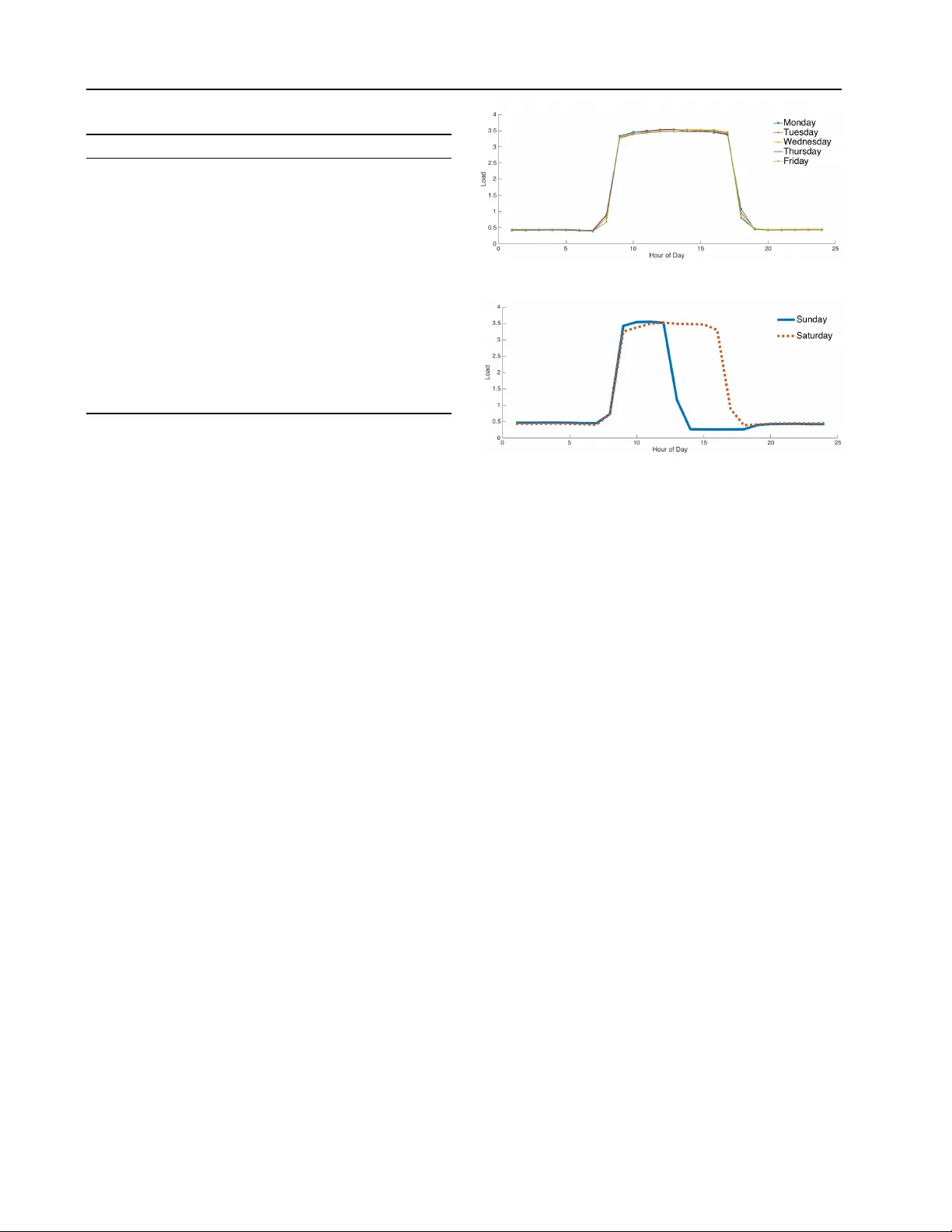
Impr oving P o wer Generation Efficiency using Deep Neural Networks Stefan Hosein S T E FA N . H O S E I N 2 @ M Y . U W I . E D U Patrick Hosein PA T R I C K . H O S E I N @ S TA . U W I . E D U The Univ ersity of the W est Indies, St. Augustine, T rinidad and T obago Abstract Recently there has been significant research on power generation, distribution and transmission efficienc y especially in the case of renewable resources. The main objecti ve is reduction of energy losses and this requires improv ements on data acquisition and analysis. In this paper we address these concerns by using consumers’ electrical smart meter readings to estimate net- work loading and this information can then be used for better capacity planning. W e com- pare Deep Neural Network (DNN) methods with traditional methods for load forecasting. Our results indicate that DNN methods outperform most traditional methods. This comes at the cost of additional computational complexity but this can be addressed with the use of cloud resources. W e also illustrate how these results can be used to better support dynamic pricing. 1. Introduction Currently , most of the energy produced worldwide uses coal or natural gas. Howe ver , much of this energy is wasted. In the United States of America, approximately 58% of energy produced is wasted ( Battaglia , 2013 ). Fur - thermore, 40% of this wasted energy is due to industrial and residential b uildings. By reducing ener gy w astage in the electric po wer industry , we reduce damage to the en vironment and reduce the dependence on fossil fuels. Short-term load forecasting (STLF) (i.e., one hour to a few weeks) can assist since, by predicting load, one can do more precise planning, supply estimation and price determination. This leads to decreased operating costs, increased profits and a more reliable electricity supply for the customer . Over the past decades of research in STLF there hav e been numerous models proposed to solve this 2016 ICML W orkshop on #Data4Good: Machine Learning in Social Good Applications , Ne w Y ork, NY , USA. Copyright by the author(s). problem. These models have been classified into classical approaches like moving average ( de Andrade & da Silva , 2009 ) and regression models ( Hong et al. , 2011 ), as well as machine learning based techniques, regression trees ( Mori & K osemura , 2001 ), support vector machines ( Niu et al. , 2006 ) and Artificial Neural Networks ( Lee et al. , 1992 ). In recent years, many deep learning methods hav e been shown to achiev e state-of-the-art performance in various areas such as speech recognition ( Hinton et al. , 2012 ), com- puter vision ( Krizhe vsky et al. , 2012 ) and natural language processing ( Collobert & W eston , 2008 ). This promise has not been demonstrated in other areas of computer science due to a lack of thorough research. Deep learning methods are representation-learning methods with multiple levels of representation obtained by composing simple but non- linear modules that each transform the representation at one lev el (starting with the raw input) into a representation at a higher , slightly more abstract lev el ( LeCun et al. , 2015 ). W ith the composition of enough such transformations, v ery complex functions can be learned. In this paper, we compare deep learning and traditional methods when applied to our STLF problem and we also provide a comprehensi ve analysis of numerous deep learn- ing models. W e then sho w how these methods can be used to assist in the pricing of electricity which can lead to less energy wastage. T o the best of our kno wledge, there is little work in such comparisons for power usage in an electrical grid. The data we use is based on one year of smart meter data collected from residential customers. W e apply each of the deep and traditional algorithms to the collected data while also noting the corresponding computational runtimes. Due to dif ferences in electricity usage between the week and the weekend, we then split the data into two new datasets: weekends and weekly data. The algorithms are applied to these ne w datasets and the results are analyzed. The results show that the deep architectures are superior to the traditional methods by ha ving the lo west error rate, but they do hav e the longest run-time. Due to space limitations we do not provide details of the traditional approaches but do pro vide references. 1 Impro ving Po wer Generation Efficiency using Deep Neural Networks T able 1. Baseline algorithms Algorithm MAPE MPE T ime (s) WMA 9.51 -1.96 100 MLR 24.25 -1.47 1 MQR 12.91 -7.63 7 R T 7.23 -1.71 15 SVR 13.65 3.16 19 2. Analysis 2.1. Data Description Our dataset consists of 8592 samples of 18 features that were collected from several households. The dataset was broken into 3 parts for training, vali dation and testing of sizes 65%, 15%, 20% respecti vely . The readings were recorded at hourly intervals throughout the year . Some of the features were electrical load readings for the previous hour , the previous two hours, the pre vious three hours, the previous day same hour , the previous day pre vious hour , the previous day previous two hours, the previous 2 days same hour , the previous 2 days previous hour , the previous 2 days previous two hours, the previous week same hour, the av erage of the past 24 hours and the average of the past 7 days. The rest of the features (which do not contain electrical load readings) are the day of the week, hour of the day , if it is a weekend, if it is a holiday , temperature and humidity . These features were selected as they are typically used for STLF . In addition, the total electrical load does not change significantly throughout the year since the households are located in a tropical country where the temperature remains fairly constant throughout the year . 2.2. Comparison Method As a preprocessing step, the data is cleaned and scaled to zero mean and unit variance. All traditional methods use cross-v alidation to determine appropriate v alues for the hyper -parameters. A random grid search was used to determine the hyper-parameters for the deep learning methods. Sev eral baseline algorithms were chosen. They include the W eighted Moving A verage (WMA) where y t +1 = αy i + β y i − 167 with α = 0 . 05 and β = 0 . 95 , Multiple Linear Regression (MLR) and quadratic regression (MQR), Regression T ree (R T) with the minimum number of branch nodes being 8, Support V ector Regression (SVR) with a linear kernel and Multilayer Perception (MLP), with the number of hidden neurons being 100. For our Deep Neural Network methods we used Deep Neural Network without pretraining (DNN-W), DNN with pretraining using Stacked Autoencoders (DNN-SA) ( Shin T able 2. DNN algorithms (subscript denotes number of layers) Algorithm 200 Epocs 400 Epocs MAPE MPE Time(s) MAPE MPE Time(s) MLP 5.62 -5.62 14 4.55 -4.54 25 DNN-W 3 2.64 1.61 30 2.50 1.98 56 DNN-W 4 5.71 -5.36 37 5.48 -5.32 72 DNN-W 5 4.40 1.79 38 5.98 5.45 69 DNN-SA 3 2.97 1.23 23 2.01 0.74 25 DNN-SA 4 2.88 0.23 29 2.37 0.79 42 DNN-SA 5 2.92 0.91 37 1.84 0.53 49 RNN 5.23 0.89 174 5.13 -0.37 359 RNN-LSTM 5.36 -1.26 880 5.27 -1.17 1528 CNN-LSTM 5.74 -3.85 1029 6.43 -5.96 1912 CNN 3.15 -3.53 799 4.60 4.23 1188 et al. , 2011 ), Recurrent Neural Networks (RNN) ( Hermans & Schrauwen , 2013 ), RNNs and Long Short T erm Memory (RRN-LSTM) ( Gers et al. , 2001 ), Con v olutional Neural Networks (CNN) ( Siripurapu , 2015 ) and CNNs and Long Short T erm Memory (CNN-LSTM)] ( Sainath et al. , 2015 ) T o ev aluate the goodness of fit of these algorithms we use the Mean Absolute Percentage Error (MAPE) defined as: MAPE = 100 n n X t =1 | y t − b y t | y t (1) where n is the number of data points, t is the particular time step, y t is the target or actual value and b y t is the predicted value. In order to determine the cost of the prediction errors (i.e. whether the prediction is above or below the actual value) the Mean Percentage Error (MPE) is used, which is defined as: MPE = 100 n n X t =1 y t − b y t y t (2) 2.3. Numerical Results W e first look at the baseline methods, (with the e xception of MLP) in T able 1 . From the table we see that MLR performs the worst, with a MAPE of 24.25%, which would indicate that the problem is not linear (see Figure 1 ). Howe ver , the R T algorithm outperforms the rest of the methods by a noticeable margin. This shows that the problem can be split into some discrete segments which would accurately forecast the load. This can be confirmed by looking at the load in Figure 1 where it is clear that, depending on the time of day , there is significant overlap of the v alue of the load between days. Thus, having a node in the R T determining the time of the day would significantly improve accuracy . The run-time for these algorithms was quite short with WMA taking the longest due to the cross-validation step where we determined all possible coefficients in steps of 2 Impro ving Po wer Generation Efficiency using Deep Neural Networks T able 3. Daily MAPE V alues Algorithm Sun Mon T ue W ed Thu Fri Sat WMA 5.71 10.05 8.87 10.24 10.74 10.37 10.67 MLR 65.46 27.61 12.55 11.39 9.01 9.38 35.59 MQR 1.17 11.92 9.88 14.24 14.11 17.11 13.24 R T 7.45 5.99 7.63 7.37 5.98 7.26 8.87 SVR 20.70 12.96 10.73 11.53 11.63 10.90 17.40 MLP 5.18 4.62 4.43 4.27 4.31 4.70 4.34 DNN-W 3 2.95 1.88 2.12 2.49 2.54 2.46 3.12 DNN-W 4 6.67 5.45 5.25 4.88 4.61 5.65 5.83 DNN-W 5 7.23 5.53 5.56 6.14 6.13 5.81 5.48 DNN-SA 3 2.29 1.84 1.76 1.97 1.87 2.03 2.35 DNN-SA 4 2.67 2.19 2.00 2.14 2.27 2.55 2.82 DNN-SA 5 2.28 1.47 1.63 1.93 1.60 1.76 2.22 RNN 5.38 5.30 4.41 5.14 5.11 5.35 5.45 RNN-LSTM 4.25 4.34 4.96 4.55 5.64 6.97 6.13 CNN-LSTM 7.79 6.86 6.04 6.05 5.65 6.44 6.21 CNN 6.39 4.20 4.27 3.32 3.87 4.18 5.03 0.05. Due to the typically long running time of DNN architec- tures, the algorithms were restricted to 200 and 400 epocs. From T able 2 , there is a clear difference when looking at the 200 epocs and the 400 epocs MAPE columns, as most of the algorithms ha ve a lo wer MAPE after running for 400 epocs when compared with 200 epocs. This is especially true for the DNN-SA 3 which saw significant drops in the MAPE. The MLP did not perform the worst in both epocs but it was always in the lower half of accuracy . This indicates that the shallow network might not be finding the patterns or structure of the data as quickly as the DNN architectures. Howe ver , it outperformed R T in both the 200 and 400 epocs. This alludes to the fact that the hidden layer is helping to capture some of the underlying dynamics that a R T cannot. Looking at the 200 epocs column, we see that DNN-W 3 performs the best with a MAPE of 2.64%. On the other hand, the most stable architecture is the DNN-SA with a MAPE consistently less than 3%. This rob ustness is shown when the epocs are increased to 400 where the DNN-SA architecture outperforms all the other methods (both the baseline and deep methods). The pretraining certainly gav e these methods a boost ov er the other methods as it guides the learning to wards basins of attraction of minima that support better generalization from the training data set ( Erhan et al. , 2010 ). RNNs, and to an extent LSTM, hav e an internal state which giv es it the ability to exhibit dynamic temporal behavior . Howe v er , they require a much longer time to compute which is evident in T able 2 since these methods had trouble mapping those underlying dynamics of the data in such a small number of epocs. CNNs do not maintain internal state, howe ver with load forecasting data, one can e xpect a fair amount of auto- correlation that requires memory . This could explain their (a) W eekday Electrical Usage (b) W eekend Electrical Usage Figure 1. Electrical Profiles somewhat lo w but unstable MAPE for 200 and 400 epocs. T aking both tables into consideration, most of the DNN architectures vastly outperform the traditional approaches, but DNNs require significantly more time to run and thus there is a trade-off. For STLF , which is a very dynamic en vironment, one cannot wait for a ne w model to complete its training stage. Hence, this is another reason we limited the number of epocs to 200 and 400. T able 2 shows that limiting the epocs did not adversely affect many of the DNN architectures as most were able to surpass the accuracy of the traditional methods (some by a lot). When selecting a model, one would hav e to determine if the length of time to run the model is worth the trade-off between accuracy and runtime. 2.4. Daily Analysis W e kno w that people ha ve dif ferent electrical usage pat- terns on weekdays when compared to weekends. This dif- ference can be seen in Figure 1 which illustrates usage for a sample home. This household uses more energy during the weekdays than on weekends. There are electrical profiles that may be opposite, i.e., where the weekend electrical load is more. Whatever the scenario, there are usually different profiles for weekdays and week ends. T o see ho w our models handle weekdays and weekends, we calculated the average MAPE for each day of the week in the test set (the 400 epoc models was used for the DNNs calculations). The av erage for each day of the week is tabulated in T able 3 . From the table, it is 3 Impro ving Po wer Generation Efficiency using Deep Neural Networks clear that most of the DNN algorithms hav e their lo west MAPE during the week. This is indicativ e that the patterns for weekdays are similar and as a result hav e more data. By ha ving more data, DNNs are better able to capture the underlying structure of the data and thus are able to predict the electrical load with greater accuracy . W eekend predictions have a higher MAPE since DNNs require a lot of data to perform accurate predictions and for weekends this data is limited. The WMA and MQR seem to have their best day on Sunday , but have a v ery poor MAPE for the rest of the days. This indicates that the models hav e an internal bias to wards Sunday and as a result fail to accurately predict the values for other days. It is clear, again, that DNNs outperform the traditional methods. 2.5. Mean Per centage Err or In this particular domain, an electricity provider will also be interested in changes of electrical load, as opposed to absolute error , in order to adjust generation accordingly , mostly because starting up additional plants takes time. This is why the Mean Percentage Error (MPE) was used. The MPE would tell that a model with a positiv e value ”under-predicts” the load while a negati ve value ”over - predicts” the actual value and they can then adjust their operations accordingly . Many of the traditional methods had predicted more elec- trical load than the actual load, including MLP . Howe ver , most of the DNNs have under-predicted the load value. Looking at the best in T able 2 , DNN-SAs MPE v alues (for 400 epocs), they are all under 1% and positive, which indicates that it under-predicts the value. Howe ver , one should not use the MPE alone. An example is RNNs which hav e a low positive MPE, howe ver it’ s MAPE in both epocs is around 5%. This indicates that RNN had a slightly larger sum of values that ”under-predicts” than ”ov er-predicts”, but its overall accuracy is not as good as other deep architectures. 2.6. Applications to Ener gy Efficiency Using the results from STLF (MAPE and MPE), a com- pany can no w accurately predict upcoming load. This would mean that a power generating compan y can now produce energy at a much more precise amount rather than producing excess energy that would be wasted. Since most of these companies use fossil fuels which are non- renew able sources of energy , we would be conserving them as well as reducing lev els of carbon dioxide released into the atmosphere and the toxic byproducts of fossil fuels. Another benefit of accurate load forecasting is that of dynamic pricing. Many residential customers pay a fixed rate per kilowatt. Dynamic pricing is an approach that allows the cost of electricity to be based on ho w expensi ve this electricity is to produce at a giv en time. The production cost is based on many factors, which in this paper , is characterized by the algorithms for STLF . By having a precise forecast of electrical load, companies no w have the ability to determine trends, especially at peak times. An example of this would be in the summer months when many people may w ant to turn on their air conditioners and thus electricity now becomes expensiv e to produce as the company could ha ve to start up additional power generating plants to account for this load. If the algorithms predict that there would be this increase in electrical load around the summer months, this w ould be reflected in the higher price that consumers would need to pay . As a result, most people would not w ant to k eep their air conditioner on all the time (as per usual) but use it only when necessary . T aking this example and adding on washing machines, lights and other appliances, we can see the immense decrease in energy that can be achiev ed on the consumer side. 3. Related W ork The area of short-term load forecasting (STLF) has been studied for many decades but deep learning has only recently seen a surge of research into its applications. Significant research has been focused on Recurrent Neu- ral Networks (RNNs). In the thesis by ( Mishra , 2008 ), RNNs was used to compare other methods for STLF . These methods included modifications of MLP by training with algorithms lik e P article Swarm Optimization, Genetic Algorithms and Artificial Immune Systems. T wo other notable papers that attempt to apply DNN for STLF are ( Busseti et al. , 2012 ) and ( Connor et al. , 1992 ). In ( Busseti et al. , 2012 ), they compare Deep Feedfow ard Neural Networks, RNNs and kernelized regression. In the paper by ( Connor et al. , 1992 ) a RNN is used for fore- casting loads and the result is compared to a Feedfo ward Neural Network. Ho we ver , a thorough comparison of various DNN architectures is lacking and any applications to dynamic pricing or energy ef ficiency is absent. 4. Conclusion In this paper , we focused on energy wastage in the electrical grid. T o achiev e this, we first needed to hav e an accurate algorithm for STLF . W ith the advent of many deep learning algorithms, we compared the accuracy of a number of deep learning methods and traditional methods. The results indi- cate that most DNN architectures achieve greater accuracy than traditional methods e ven when the data is split into weekdays and weekends. Howe ver such algorithms hav e longer runtimes. W e also discussed how these algorithms can hav e a significant impact in conserving energy at both the producer and consumer lev els. 4 Impro ving Po wer Generation Efficiency using Deep Neural Networks References Battaglia, Sarah. Us now leads in ener gy waste, 2013. URL http://www. theenergycollective.com/sbattaglia/ 193441/us- most- energy- waste . Busseti, Enzo, Osband, Ian, and W ong, Scott. Deep learning for time series modeling. T echnical report, Stanford, 2012. Collobert, Ronan and W eston, Jason. A unified architecture for natural language processing: Deep neural networks with multitask learning. In Pr oceedings of the 25th International Confer ence on Mac hine Learning , 2008. Connor , Jerome, Atlas, Les E., and Martin, Douglas R. Recurrent networks and narma modeling. In Advances in Neural Information Pr ocessing Systems 4 . 1992. de Andrade, L.C.M. and da Silva, I.N. V ery short-term load forecasting based on arima model and intelligent systems. In Intelligent System Applications to P ower Systems, 2009. ISAP ’09. 15th International Conference on , 2009. Erhan, Dumitru, Bengio, Y oshua, Courville, Aaron, Manzagol, Pierre-Antoine, V incent, Pascal, and Bengio, Samy . Why does unsupervised pre-training help deep learning? J. Mach. Learn. Res. , 11, March 2010. Gers, Felix A., Eck, Douglas, and Schmidhuber , J ¨ urgen. Artificial Neural Networks — ICANN 2001: International Conference V ienna, Austria, August 21– 25, 2001 Pr oceedings , chapter Applying LSTM to Time Series Predictable through T ime-W indow Approaches. 2001. Hermans, Michiel and Schrauwen, Benjamin. T raining and analysing deep recurrent neural networks. In Advances in Neural Information Pr ocessing Systems 26 , pp. 190– 198. 2013. Hinton, Geoffre y , Deng, Li, Y u, Dong, rahman Mohamed, Abdel, Jaitly , Na vdeep, Senior , Andrew , V anhoucke, V incent, Nguyen, Patrick, Dahl, T ara Sainath George, and Kingsbury , Brian. Deep neural networks for acoustic modeling in speech recognition. IEEE Signal Pr ocessing Magazine , 2012. Hong, T ao, W ang, Pu, and W illis, H.L. A na ¨ ıve multiple linear regression benchmark for short term load forecasting. In P ower and Ener gy Society General Meeting, 2011 IEEE , 2011. Krizhevsk y , Alex, Sutske v er , Ilya, and Hinton, Geof frey E. Imagenet classification with deep con v olutional neural networks. In Advances in Neural Information Pr ocessing Systems 25 , pp. 1097–1105. 2012. LeCun, Y ann, Bengio, Y oshua, and Hinton, Geof frey . Deep learning. Nature , 2015. Lee, K.Y ., Cha, Y .T ., and Park, J.H. Short-term load forecasting using an artificial neural network. P ower Systems, IEEE T ransactions on , 1992. Mishra, Sanjob . Long short-term memory in recurrent neural networks. Master’ s thesis, National Institute Of T echnology Rourkela, 2008. Mori, H. and Kosemura, N. Optimal regression tree based rule discovery for short-term load forecasting. In P ower Engineering Society W inter Meeting, 2001. IEEE , 2001. Niu, Dong-Xiao, W ang, Qiang, and Li, Jin-Chao. Advances in Machine Learning and Cybernetics: 4th International Confer ence , chapter Short T erm Load Forecasting Model Based on Support V ector Machine. 2006. Sainath, T . N., V in yals, O., Senior, A., and Sak, H. Con v olutional, long short-term memory , fully connected deep neural networks. In 40th IEEE International Confer ence on Acoustics, Speech and Signal Pr ocessing , 2015. Shin, Hoo-Chang, Orton, M., Collins, D.J., Doran, S., and Leach, M.O. Autoencoder in time-series analysis for unsupervised tissues characterisation in a large unlabelled medical image dataset. In Machine Learning and Applications and W orkshops (ICMLA), 2011 10th International Confer ence on , 2011. Siripurapu, Ashwin. Conv olutional networks for stock trading. T echnical report, Stanford University , 2015. 5