Auxiliary Deep Generative Models

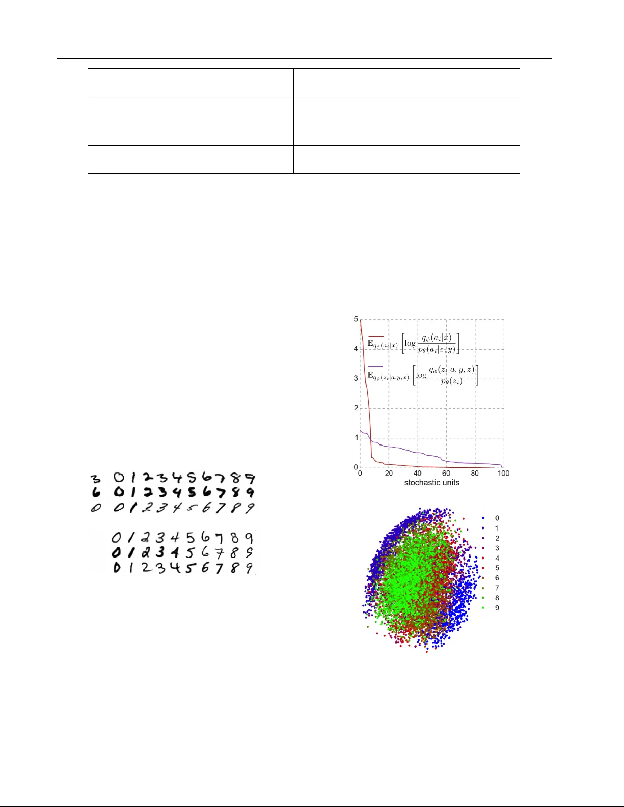
A uxiliary Deep Generativ e Models Lars Maaløe 1 L A R S M A @ D T U . D K Casper Kaae Sønderby 2 C A S P E R K A A E @ G M A I L . C O M Søren Kaae Sønderby 2 S K A A E S O N D E R B Y @ G M A I L . C O M Ole Winther 1 , 2 O LW I @ D T U . D K 1 Department of Applied Mathematics and Computer Science, T echnical Univ ersity of Denmark 2 Bioinformatics Centre, Department of Biology , Univ ersity of Copenhagen Abstract Deep generativ e models parameterized by neu- ral networks ha ve recently achie v ed state-of- the-art performance in unsupervised and semi- supervised learning. W e extend deep genera- tiv e models with auxiliary variables which im- prov es the variational approximation. The aux- iliary variables leave the generative model un- changed but mak e the v ariational distribution more expressiv e. Inspired by the structure of the auxiliary variable we also propose a model with two stochastic layers and skip connections. Our findings suggest that more expressiv e and prop- erly specified deep generative models con ver ge faster with better results. W e show state-of-the- art performance within semi-supervised learning on MNIST , SVHN and NORB datasets. 1. Introduction Stochastic backpropagation, deep neural networks and ap- proximate Bayesian inference have made deep generati ve models practical for large scale problems ( Kingma , 2013 ; Rezende et al. , 2014 ), but typically they assume a mean field latent distribution where all latent variables are in- dependent. This assumption might result in models that are incapable of capturing all dependencies in the data. In this paper we show that deep generativ e models with more expressi v e v ariational distrib utions are easier to optimize and hav e better performance. W e increase the flexibility of the model by introducing auxiliary variables ( Agakov and Barber , 2004 ) allowing for more comple x latent distribu- tions. W e demonstrate the benefits of the increased flexibil- ity by achieving state-of-the-art performance in the semi- supervised setting for the MNIST ( LeCun et al. , 1998 ), Pr oceedings of the 33 rd International Confer ence on Mac hine Learning , New Y ork, NY , USA, 2016. JMLR: W&CP volume 48. Copyright 2016 by the author(s). SVHN ( Netzer et al. , 2011 ) and NORB ( LeCun et al. , 2004 ) datasets. Recently there hav e been significant improv ements within the semi-supervised classification tasks. Kingma et al. ( 2014 ) introduced a deep generativ e model for semi- supervised learning by modeling the joint distribution ov er data and labels. This model is difficult to train end-to-end with more than one layer of stochastic latent variables, but coupled with a pretrained feature extractor it performs well. Lately the Ladder network ( Rasmus et al. , 2015 ; V alpola , 2014 ) and virtual adversarial training (V A T) ( Miyato et al. , 2015 ) have improv ed the performance further with end-to- end training. In this paper we train deep generativ e models with mul- tiple stochastic layers. The Auxiliary Deep Generative Models (ADGM) utilize an extra set of auxiliary latent vari- ables to increase the flexibility of the variational distribu- tion (cf. Sec. 2.2 ). W e also introduce a slight change to the ADGM, a 2-layered stochastic model with skip con- nections, the Skip Deep Generative Model (SDGM) (cf. Sec. 2.4 ). Both models are trainable end-to-end and offer state-of-the-art performance when compared to other semi- supervised methods. In the paper we first introduce toy data to demonstrate that: (i) The auxiliary v ariable models can fit comple x la- tent distributions and thereby improv e the variational lower bound (cf. Sec. 4.1 and 4.3 ). (ii) By fitting a complex half-moon dataset using only six labeled data points the ADGM utilizes the data mani- fold for semi-supervised classification (cf. Sec. 4.2 ). For the benchmark datasets we sho w (cf. Sec. 4.4 ): (iii) State-of-the-art results on several semi-supervised classification tasks. (iv) That multi-layered deep generativ e models for semi- supervised learning are trainable end-to-end without pre-training or feature engineering. A uxiliary Deep Generati ve Models 2. A uxiliary deep generative models Recently Kingma ( 2013 ); Rezende et al. ( 2014 ) hav e cou- pled the approach of variational inference with deep learn- ing giving rise to powerful probabilistic models constructed by an inference neural netw ork q ( z | x ) and a generativ e neural network p ( x | z ) . This approach can be perceiv ed as a variational equiv alent to the deep auto-encoder , in which q ( z | x ) acts as the encoder and p ( x | z ) the decoder . Ho w- ev er , the dif ference is that these models ensures efficient inference over continuous distributions in the latent space z with automatic relev ance determination and regulariza- tion due to the KL-diver gence. Furthermore, the gradients of the variational upper bound are easily defined by back- propagation through the network(s). T o keep the computa- tional requirements low the variational distrib ution q ( z | x ) is usually chosen to be a diagonal Gaussian, limiting the expressi v e power of the inference model. In this paper we propose a variational auxiliary vari- able approach ( Agako v and Barber , 2004 ) to improv e the variational distribution: The generati ve model is ex- tended with variables a to p ( x, z, a ) such that the original model is in v ariant to marginalization over a : p ( x, z , a ) = p ( a | x, z ) p ( x, z ) . In the variational distribution, on the other hand, a is used such that marginal q ( z | x ) = R q ( z | a, x ) p ( a | x ) da is a general non-Gaussian distribution. This hierarchical specification allows the latent variables to be correlated through a , while maintaining the computa- tional efficienc y of fully factorized models (cf. Fig. 1 ). In Sec. 4.1 we demonstrate the expressi ve po wer of the infer- ence model by fitting a complex multimodal distrib ution. 2.1. V ariational auto-encoder The variational auto-encoder (V AE) has recently been in- troduced as a po werful method for unsupervised learning. Here a latent variable generativ e model p θ ( x | z ) for data x is parameterized by a deep neural network with parameters θ . The parameters are inferred by maximizing the varia- tional lower bound of the lik elihood − P i U V AE ( x i ) with log p ( x ) = log Z z p ( x, z ) dz ≥ E q φ ( z | x )  log p θ ( x | z ) p θ ( z ) q φ ( z | x )  (1) ≡ −U V AE ( x ) . The inference model q φ ( z | x ) is parameterized by a second deep neural network. The inference and generative param- eters, θ and φ , are jointly trained by optimizing Eq. 1 with stochastic gradient ascent, where we use the reparameter- ization trick for backpropagation through the Gaussian la- tent variables ( Kingma , 2013 ; Rezende et al. , 2014 ). y z a x (a) Generativ e model P . y z a x (b) Inference model Q . Figure 1. Probabilistic graphical model of the ADGM for semi- supervised learning. The incoming joint connections to each vari- able are deep neural networks with parameters θ and φ . 2.2. A uxiliary variables W e propose to extend the v ariational distrib ution with aux- iliary variables a : q ( a, z | x ) = q ( z | a, x ) q ( a | x ) such that the marginal distribution q ( z | x ) can fit more complicated pos- teriors p ( z | x ) . In order to hav e an unchanged generative model, p ( x | z ) , it is required that the joint mode p ( x, z , a ) giv es back the original p ( x, z ) under marginalization over a , thus p ( x, z , a ) = p ( a | x, z ) p ( x, z ) . Auxiliary variables are used in the EM algorithm and Gibbs sampling and hav e pre viously been considered for v ariational learning by Agakov and Barber ( 2004 ). Concurrent with this work Ranganath et al. ( 2015 ) have proposed to make the param- eters of the v ariational distribution stochastic, which leads to a similar model. It is important to note that in order not to fall back to the original V AE model one has to re- quire p ( a | x, z ) 6 = p ( a ) , see Agakov and Barber ( 2004 ) and App. A . The auxiliary V AE lower bound becomes log p ( x ) = log Z a Z z p ( x, a, z ) dadz ≥ E q φ ( a,z | x )  log p θ ( a | z , x ) p θ ( x | z ) p ( z ) q φ ( a | x ) q φ ( z | a, x )  (2) ≡ −U A V AE ( x ) . with p θ ( a | z , x ) and q φ ( a | x ) diagonal Gaussian distrib u- tions parameterized by deep neural networks. 2.3. Semi-supervised learning The main focus of this paper is to use the auxiliary ap- proach to build semi-supervised models that learn clas- sifiers from labeled and unlabeled data. T o encom- pass the class information we introduce an extra la- tent v ariable y . The generati v e model P is defined as p ( y ) p ( z ) p θ ( a | z , y , x ) p θ ( x | y , z ) (cf. Fig. 1a ): p ( z ) = N ( z | 0 , I) , (3) p ( y ) = Cat ( y | π ) , (4) p θ ( a | z , y , x ) = f ( a ; z , y , x, θ ) , (5) p θ ( x | z , y ) = f ( x ; z , y , θ ) , (6) A uxiliary Deep Generati ve Models where a , y , z are the auxiliary variable, class label, and la- tent features, respecti vely . Cat ( · ) is a multinomial distribu- tion, where y is treated as a latent v ariable for the unlabeled data points. In this study we only experimented with cate- gorical labels, howe v er the method applies to other distri- butions for the latent v ariable y . f ( x ; z , y , θ ) is iid categori- cal or Gaussian for discrete and continuous observations x . p θ ( · ) are deep neural networks with parameters θ . The in- ference model is defined as q φ ( a | x ) q φ ( z | a, y , x ) q φ ( y | a, x ) (cf. Fig. 1b ): q φ ( a | x ) = N ( a | µ φ ( x ) , diag ( σ 2 φ ( x ))) , (7) q φ ( y | a, x ) = Cat ( y | π φ ( a, x )) , (8) q φ ( z | a, y , x ) = N ( z | µ φ ( a, y , x ) , diag ( σ 2 φ ( a, y , x ))) . (9) In order to model Gaussian distributions p θ ( a | z , y , x ) , p θ ( x | z , y ) , q φ ( a | x ) and q φ ( z | a, y , x ) we define two sepa- rate outputs from the top deterministic layer in each deep neural network, µ φ ∨ θ ( · ) and log σ 2 φ ∨ θ ( · ) . From these out- puts we are able to approximate the expectations E by ap- plying the reparameterization trick. The key point of the ADGM is that the auxiliary unit a introduce a latent feature extractor to the inference model giving a richer mapping between x and y . W e can use the classifier ( 9 ) to compute probabilities for unlabeled data x u being part of each class and to retrie ve a cross-entropy er- ror estimate on the labeled data x l . This can be used in cohesion with the variational lo wer bound to define a good objectiv e function in order to train the model end-to-end. V A R I A T I O NA L L OW E R B O U N D W e optimize the model by maximizing the lo wer bound on the likelihood (cf. App. B for more details). The v ariational lower bound on the mar ginal likelihood for a single labeled data point is log p ( x, y ) = log Z a Z z p ( x, y , a, z ) dz da ≥ E q φ ( a,z | x,y )  log p θ ( x, y , a, z ) q φ ( a, z | x, y )  (10) ≡ −L ( x, y ) , with q φ ( a, z | x, y ) = q φ ( a | x ) q φ ( z | a, y , x ) . For unlabeled data we further introduce the variational distribution for y , q φ ( y | a, x ) : log p ( x ) = log Z a Z y Z z p ( x, y , a, z ) dz dy da ≥ E q φ ( a,y ,z | x )  log p θ ( x, y , a, z ) q φ ( a, y , z | x )  (11) ≡ −U ( x ) , with q φ ( a, y , z | x ) = q φ ( z | a, y , x ) q φ ( y | a, x ) q φ ( a | x ) . The classifier ( 9 ) appears in −U ( x u ) , but not in −L ( x l , y l ) . The classification accuracy can be improv ed by introducing an explicit classification loss for labeled data: L l ( x l , y l ) = (12) L ( x l , y l ) + α · E q φ ( a | x l ) [ − log q φ ( y l | a, x l )] , where α is a weight between generati ve and discriminati ve learning. The α parameter is set to β · N l + N u N l , where β is a scaling constant, N l is the number of labeled data points and N u is the number of unlabeled data points. The objec- tiv e function for labeled and unlabeled data is J = X ( x l ,y l ) L l ( x l , y l ) + X ( x u ) U ( x u ) . (13) 2.4. T wo stochastic layers with skip connections Kingma et al. ( 2014 ) proposed a model with two stochas- tic layers but were unable to make it con ver ge end- to-end and instead resorted to layer-wise training. In our preliminary analysis we also found that this model: p θ ( x | z 1 ) p θ ( z 1 | z 2 , y ) p ( z 2 ) p ( y ) failed to conv er ge when trained end-to-end. On the other hand, the auxil- iary model can be made into a two-layered stochastic model by simply rev ersing the arrow between a and x in Fig. 1a . W e would expect that if the auxiliary model works well in terms of conv er gence and perfor- mance then this two-layered model ( a is no w part of the generativ e model): p θ ( x | y , a, z ) p θ ( a | z , y ) p ( z ) p ( y ) should work even better because it is a more flexible genera- tiv e model. The variational distribution is unchanged: q φ ( z | y , x, a ) q φ ( y | a, x ) q φ ( a | x ) . W e call this the Skip Deep Generative Model (SDGM) and test it alongside the auxil- iary model in the benchmarks (cf. Sec. 4.4 ). 3. Experiments The SDGM and ADGM are each parameterized by 5 neu- ral networks (NN): (1) auxiliary inference model q φ ( a | x ) , (2) latent inference model q φ ( z | a, y , x ) , (3) classification model q φ ( y | a, x ) , (4) generati ve model p θ ( a |· ) , and (5) the generativ e model p θ ( x |· ) . The neural networks consists of M fully connected hidden layers with h j denoting the output of a layer j = 1 , ..., M . All hidden layers use rectified linear acti v ation functions. T o compute the approximations of the stochastic variables we place two independent output layers after h M , µ and log σ 2 . In a forward-pass we are propagating the input x through the neural network by h M = NN ( x ) (14) µ = Linear ( h M ) (15) log σ 2 = Linear ( h M ) , (16) A uxiliary Deep Generati ve Models with Linear denoting a linear activ ation function. W e then approximate the stochastic variables by applying the repa- rameterization trick using the µ and log σ 2 outputs. In the unsupervised toy example (cf. Sec. 4.1 ) we ap- plied 3 hidden layers with dim( h ) = 20 , dim( a ) = 4 and dim( z ) = 2 . For the semi-supervised toy example (cf. Sec. 4.2 ) we used two hidden layers of dim( h ) = 100 and dim( a, z ) = 10 . For all the benchmark experiments (cf. Sec. 4.4 ) we parameterized the deep neural networks with two fully connected hidden layers. Each pair of hidden layers was of size dim( h ) = 500 or dim( h ) = 1000 with dim( a, z ) = 100 or dim( a, z ) = 300 . The generative model was p ( y ) p ( z ) p θ ( a | z , y ) p θ ( x | z , y ) for the ADGM and the SDGM had the augmented p θ ( x | a, z , y ) . Both ha ve unchanged inference models (cf. Fig. 1b ). All parameters are initialized using the Glorot and Bengio ( 2010 ) scheme. The expectation ov er the a and z variables were performed by Monte Carlo sampling using the repa- rameterization trick ( Kingma , 2013 ; Rezende et al. , 2014 ) and the av erage ov er y by exact enumeration so E q φ ( a,y ,z | x ) [ f ( a, x, y , z )] ≈ (17) 1 N samp N samp X i X y q φ ( y | a i , x ) f ( a i , x, y , z y i ) , with a i ∼ q ( a | x ) and z y i ∼ q ( z | a, y , x ) . For training, we ha ve used the Adam ( Kingma and Ba , 2014 ) optimization framew ork with a learning rate of 3e- 4, e xponential decay rate for the 1st and 2nd moment at 0 . 9 and 0 . 999 , respecti v ely . The β constant was between 0 . 1 and 2 throughout the experiments. The models are implemented in Python using Theano ( Bastien et al. , 2012 ), Lasagne ( Dieleman et al. , 2015 ) and Parmesan libraries 1 . For the MNIST dataset we hav e combined the training set of 50000 examples with the validation set of 10000 exam- ples. The test set remained as is. W e used a batch size of 200 with half of the batch always being the 100 labeled samples. The labeled data are chosen randomly , but dis- tributed evenly across classes. T o speed up training, we remov ed the columns with a standard deviation below 0 . 1 resulting in an input size of dim( x ) = 444 . Before each epoch the normalized MNIST images were binarized by sampling from a Bernoulli distribution with mean parame- ter set to the pixel intensities. For the SVHN dataset we used the vectorized and cropped training set dim( x ) = 3072 with classes from 0 to 9 , com- 1 Implementation is av ailable in a repository named auxiliary- deep-generativ e-models on github.com . bined with the extra set resulting in 604388 data points. The test set is of size 26032 . W e trained on the small NORB dataset consisting of 24300 training samples and an equal amount of test samples distrib uted across 5 classes: animal , human , plane , truck , car . W e normalized all NORB images following Miyato et al. ( 2015 ) using image pairs of 32 x 32 resulting in a vectorized input of dim( x ) = 2048 . The labeled subsets consisted of 1000 e venly dis- tributed labeled samples. The batch size for SVHN was 2000 and for NORB 200 , where half of the batch was la- beled samples. T o av oid the phenomenon on modeling dis- cretized values with a real-valued estimation ( Uria et al. , 2013 ), we added uniform noise between 0 and 1 to each pixel value. W e normalized the NORB dataset by 256 and the SVHN dataset by the standard deviation on each color channel. Both datasets were assumed Gaussian distributed for the generativ e models p θ ( x |· ) . 4. Results In this section we present two toy examples that shed light on how the auxiliary v ariables improv e the distribution fit. Thereafter we in vestigate the unsupervised generativ e log-likelihood performance followed by semi-supervised classification performance on sev eral benchmark datasets. W e demonstrate state-of-the-art performance and sho w that adding auxiliary variables increase both classification per- formance and con v ergence speed (cf. Sec. 3 for details). 4.1. Beyond Gaussian latent distrib utions In v ariational auto-encoders the inference model q φ ( z | x ) is parameterized as a fully factorized Gaussian. W e demon- strate that the auxiliary model can fit complicated posterior distributions for the latent space. T o do this we consider the 2D potential model p ( z ) = exp( U ( z )) / Z ( Rezende and Mohamed , 2015 ) that leads to the bound log Z ≥ E q φ ( a,z )  log exp( U ( z )) p θ ( a | z ) q φ ( a ) q φ ( z | a )  . (18) Fig. 2a shows the true posterior and Fig. 2b shows a den- sity plot of z samples from a ∼ q φ ( a ) and z ∼ q φ ( z | a ) from a trained ADGM. This is similar to the findings of Rezende and Mohamed ( 2015 ) in which they demonstrate that by using normalizing flows the y can fit complicated posterior distributions. The most frequent solution found in optimization is not the one shown, but one where Q fits only one of the two equiv alent modes. The one and two mode solution will have identical values of the bound so it is to be e xpected that the simpler single mode solution will be easier to infer . A uxiliary Deep Generati ve Models (a) (b) (c) (d) Figure 2. (a) True posterior of the prior p ( z ) . (b) The approximation q φ ( z | a ) q φ ( a ) of the ADGM. (c) Prediction on the half-moon data set after 10 epochs with only 3 labeled data points (black) for each class. (d) PCA plot on the 1st and 2nd principal component of the corresponding auxiliary latent space. 4.2. Semi-supervised learning on tw o half-moons T o exemplify the po wer of the ADGM for semi- supervised learning we hav e generated a 2D synthetic dataset consisting of two half-moons (top and bot- tom), where ( x top , y top ) = ( cos ([0 , π ]) , sin ([0 , π ])) and ( x bottom , y bottom ) = (1 − cos ([0 , π ]) , 1 − sin ([0 , π ]) − 0 . 5) , with added Gaussian noise. The training set contains 1e4 samples divided into batches of 100 with 3 labeled data points in each class and the test set contains 1e4 samples. A good semi-supervised model will be able to learn the data manifold for each of the half-moons and use this together with the limited labeled information to build the classifier . The ADGM conv erges close to 0% classification error in 10 epochs (cf. Fig. 2c ), which is much faster than an equi v- alent model without the auxiliary variable that con verges in more than 100 epochs. When in v estigating the auxiliary variable we see that it finds a discriminating internal repre- sentation of the data manifold and thereby aids the classifier (cf. Fig. 2d ). 4.3. Generative log-lik elihood perf ormance W e ev aluate the generativ e performance of the unsuper- vised auxiliary model, A V AE, using the MNIST dataset. The inference and generativ e models are defined as q φ ( a, z | x ) = q φ ( a 1 | x ) q φ ( z 1 | a 1 , x ) (19) L Y i =2 q φ ( a i | a i − 1 , x ) q φ ( z i | a i , z i − 1 ) , p θ ( x, a, z ) = p θ ( x | z 1 ) p ( z L ) p θ ( a L | z L ) (20) L − 1 Y i =1 p θ ( z i | z i +1 ) p θ ( a i | z ≥ i ) . where L denotes the number of stochastic layers. W e report the lower bound from Eq. ( 2 ) for 5000 impor- tance weighted samples and use the same training and pa- rameter settings as in Sønderby et al. ( 2016 ) with warm- up 2 , batch normalization and 1 Monte Carlo and IW sample for training. ≤ log p ( x ) V A E + NF, L = 1 ( R E ZE N D E A N D M O HA M E D , 2 0 15 ) − 85 . 10 I W A E , L = 1 , I W = 1 ( B UR DA E T A L . , 2 0 1 5 ) − 86 . 76 I W A E , L = 1 , I W = 5 0 ( B U RD A E T A L . , 2 0 1 5 ) − 84 . 78 I W A E , L = 2 , I W = 1 ( B UR DA E T A L . , 2 0 1 5 ) − 85 . 33 I W A E , L = 2 , I W = 5 0 ( B U RD A E T A L . , 2 0 1 5 ) − 82 . 90 V A E + VG P , L = 2 ( T R AN E T A L . , 2 0 1 5 ) − 81 . 90 L V A E , L = 5 , I W = 1 ( S Ø N DE R B Y E T A L . , 2 0 1 6 ) − 82 . 12 L V A E , L = 5 , F T, I W = 1 0 ( S ØN D E R BY E T A L . , 2 0 1 6 ) − 81 . 74 A U X IL I A RY V A E ( A V A E ) , L = 1 , I W = 1 − 84 . 59 A U X IL I A RY V A E ( A V A E ) , L = 2 , I W = 1 − 82 . 97 T able 1. Unsupervised test log-likelihood on permutation inv ari- ant MNIST for the normalizing flo ws V AE (V AE+NF), impor- tance weighted auto-encoder (IW AE), v ariational Gaussian pro- cess V AE (V AE+VGP) and Ladder V AE (L V AE) with FT denot- ing the finetuning procedure from Sønderby et al. ( 2016 ), IW the importance weighted samples during training, and L the number of stochastic latent layers z 1 , .., z L . W e ev aluate the ne gati ve log-likelihood for the 1 and 2 lay- ered A V AE. W e found that w arm-up was crucial for acti v a- tion of the auxiliary v ariables. T able 1 shows log-likelihood scores for the permutation in v ariant MNIST dataset. The methods are not directly comparable, except for the Lad- der V AE (L V AE) ( Sønderby et al. , 2016 ), since the train- ing is performed differently . Howe v er , they gi v e a good indication on the expressi ve power of the auxiliary v ari- able model. The A V AE is performing better than the V AE with normalizing flo ws ( Rezende and Mohamed , 2015 ) and the importance weighted auto-encoder with 1 IW sample ( Burda et al. , 2015 ). The results are also comparable to the Ladder V AE with 5 latent layers ( Sønderby et al. , 2016 ) and variational Gaussian process V AE ( Tran et al. , 2015 ). As sho wn in Burda et al. ( 2015 ) and Sønderby et al. ( 2016 ) increasing the IW samples and annealing the learning rate will likely increase the log-likelihood. 2 T emperature on the KL-div ergence going from 0 to 1 within the first 200 epochs of training. A uxiliary Deep Generati ve Models M N I S T S V H N N O R B 100 L A B E L S 1000 L A B E L S 1000 L A B E L S M 1 + T S VM ( K I N G M A E T A L . , 2 0 1 4 ) 11 . 82 % ( ± 0 . 25 ) 55 . 33 % ( ± 0 . 11 ) 18 . 79 % ( ± 0 . 05 ) M 1 + M 2 ( K I N G MA E T A L . , 2 0 1 4 ) 3 . 33 % ( ± 0 . 14 ) 36 . 02 % ( ± 0 . 10 ) - V A T ( M I Y ATO E T A L . , 2 0 1 5 ) 2 . 12 % 24 . 63 % 9 . 88 % L A D D ER N E T W O R K ( R A S M U S E T A L . , 2 0 1 5 ) 1 . 06 % ( ± 0 . 37 ) - - A U X I L IA RY D E E P G E N E R A T I V E M O D E L ( A D G M ) 0 .9 6 % ( ± 0 . 02 ) 22 . 86 % 10 . 06 % ( ± 0 . 05 ) S K I P D E E P G E N E R A T I V E M O D E L ( S D G M ) 1 . 32 % ( ± 0 . 07 ) 1 6 . 6 1 % ( ± 0 . 24 ) 9 . 4 0 % ( ± 0 . 04 ) T able 2. Semi-supervised test error % benchmarks on MNIST , SVHN and NORB for randomly labeled and ev enly distributed data points. The lower section demonstrates the benchmarks of the contrib ution of this article. 4.4. Semi-supervised benchmarks M N I S T E X P E R I M E N T S T able 2 shows the performance of the ADGM and SDGM on the MNIST dataset. The ADGM’ s con ver gence to around 2% is f ast (around 200 epochs), and from that point the con vergence speed declines and finally reaching 0 . 96 % (cf. Fig. 5 ). The SDGM shows close to similar perfor- mance and prov es more stable by speeding up conv ergence, due to its more advanced generati ve model. W e achiev ed the best results on MNIST by performing multiple Monte Carlo samples for a ∼ q φ ( a | x ) and z ∼ q φ ( z | a, y , x ) . A good explorati ve estimate of the models ability to com- prehend the data manifold, or in other words be as close to the posterior distribution as possible, is to ev aluate the generativ e model. In Fig. 3a we sho w ho w the SDGM, trained on only 100 labeled data points, has learned to sep- arate style and class information. Fig 3b shows random samples from the generativ e model. (a) (b) Figure 3. MNIST analogies. (a) Forw ard propagating a data point x (left) through q φ ( z | a, x ) and generate samples p θ ( x | y j , z ) for each class label y j (right). (b) Generating a sample for each class label from random generated Gaussian noise; hence with no use of the inference model. Fig. 4a demonstrate the information contribution from the stochastic unit a i and z j (subscripts i and j denotes a unit) in the SDGM as measured by the average over the test set of the KL-di ver gence between the variational distribution and the prior . Units with little information content will be close to the prior distribution and the KL-diver gence term will thus be close to 0. The number of clearly acti vated units in z and a is quite low ∼ 20 , b ut there is a tail of slightly acti ve units, similar results hav e been reported by Burda et al. ( 2015 ). It is still e vident that we hav e informa- tion flowing through both v ariables though. Fig. 2d and 4b shows clustering in the auxiliary space for both the ADGM and SDGM respectiv ely . (a) (b) Figure 4. SDGM trained on 100 labeled MNIST . (a) The KL- div ergence for units in the latent variables a and z calculated by the difference between the approximated value and its prior . (b) PCA on the 1st and 2nd principal component of the auxiliary la- tent space. A uxiliary Deep Generati ve Models Figure 5. 100 labeled MNIST classification error % evaluated ev- ery 10 epochs between equally optimized SDGM, ADGM, M2 ( Kingma et al. , 2014 ) and an ADGM with a deterministic auxil- iary variable. In order to in vestigate whether the stochasticity of the aux- iliary variable a or the network depth is essential to the models performance, we constructed an ADGM with a de- terministic auxiliary variable. Furthermore we also imple- mented the M2 model of Kingma et al. ( 2014 ) using the exact same hyperparameters as for learning the ADGM. Fig. 5 shows how the ADGM outperforms both the M2 model and the ADGM with deterministic auxiliary vari- ables. W e found that the con ver gence of the M2 model was highly unstable; the one sho wn is the best obtained. S V H N & N O R B E X P E R I M E N T S From T able 2 we see how the SDGM outperforms V A T with a relative reduction in error rate of more than 30 % on the SVHN dataset. W e also tested the model performance, when we omitted the SVHN extra set from training. Here we achie ved a classification error of 29 . 82 %. The impro ve- ments on the NORB dataset was not as significant as for SVHN with the ADGM being slightly worse than V A T and the SDGM being slightly better than V A T . On SVHN the model trains to around 19 % classification error in 100 epochs followed by a decline in con v ergence speed. The NORB dataset is a significantly smaller dataset and the SDGM conv er ges to around 12 % in 100 epochs. W e also trained the NORB dataset on single images as op- posed to image pairs (half the dataset) and achie v ed a clas- sification error around 13 % in 100 epochs. For Gaussian input distributions, like the image data of SVHN and NORB, we found the SDGM to be more sta- ble than the ADGM. 5. Discussion The ADGM and SDGM are po werful deep generati ve mod- els with relati vely simple neural network architectures. They are trainable end-to-end and since they follow the principles of v ariational inference there are multiple im- prov ements to consider for optimizing the models like us- ing the importance weighted bound or adding more lay- ers of stochastic variables. Furthermore we have only pro- posed the models using a Gaussian latent distribution, but the model can easily be extended to other distrib utions ( Ranganath et al. , 2014 ; 2015 ). One way of approaching the stability issues of the ADGM, when training on Gaussian input distributions x is to add a temperatur e weighting between discriminative and stochastic learning on the KL-di ver gence for a and z when estimating the variational lo wer bound ( Sønderby et al. , 2016 ). W e find similar problems for the Gaussian input dis- tributions in v an den Oord et al. ( 2016 ), where the y restrict the dataset to ordinal values in order to apply a softmax function for the output of the generative model p ( x |· ) . This discretization of data is also a possible solution. Another potential stabilizer is to add batch normalization ( Ioffe and Szegedy , 2015 ) that will ensure normalization of each out- put batch of a fully connected hidden layer . A downside to the semi-supervised variational framework is that we are summing ov er all classes in order to e v aluate the v ariational bound for unlabeled data. This is a com- putationally costly operation when the number of classes grow . In this sense, the Ladder network has an advantage. A possible extension is to sample y when calculating the unlabeled lo wer bound −U ( x u ) , b ut this may result in gra- dients with high variance. The framew ork is implemented with fully connected layers. V AEs hav e proven to work well with con volutional layers so this could be a promising step to further improv e the performance. Finally , since we expect that the variational bound found by the auxiliary v ariable method is quite tight, it could be of interest to see whether the bound for p ( x, y ) may be used for classification in the Bayes classifier man- ner p ( y | x ) ∝ p ( x, y ) . 6. Conclusion W e hav e introduced a nov el framew ork for making the vari- ational distributions used in deep generative models more expressi v e. In tw o toy examples and the benchmarks we in- vestigated how the framework uses the auxiliary variables to learn better variational approximations. Finally we have demonstrated that the frame work gi ves state-of-the-art per - formance in a number of semi-supervised benchmarks and is trainable end-to-end. A uxiliary Deep Generati ve Models A. A uxiliary model specification In this appendix we study the theoretical optimum of the auxiliary v ariational bound found by functional deri vati ves of the v ariational objective. In practice we will resort to restricted deep network parameterized distributions. But this analysis nevertheless shed some light on the proper- ties of the optimum. Without loss of generality we con- sider only auxiliary a and latent z : p ( a, z ) = p ( z ) p ( a | z ) , p ( z ) = f ( z ) / Z and q ( a, z ) = q ( z | a ) q ( a ) . The results can be e xtended to the full semi-supervised setting without changing the ov erall conclusion. The variational bound for the auxiliary model is log Z ≥ E q ( a,z )  log f ( z ) p ( a | z ) q ( z | a ) q ( a )  . (21) W e can now take the functional deri vati ve of the bound with respect to p ( a | z ) . This giv es the optimum p ( a | z ) = q ( a, z ) /q ( z ) , which in general is intractable because it re- quires marginalization: q ( z ) = R q ( z | a ) q ( a ) da . One may also restrict the generati ve model to an unin- formed a -model: p ( a, z ) = p ( z ) p ( a ) . Optimizing with respect to p ( a ) we find p ( a ) = q ( a ) . When we insert this solution into the variational bound we get Z q ( a ) E q ( z | a )  log f ( z ) q ( z | a )  da . (22) The solution to the optimization with respect to q ( a ) will simply be a δ -function at the value of a that optimizes the variational bound for the z -model. So we fall back to a model for z without the auxiliary as also noted by Agako v and Barber ( 2004 ). W e have tested the uninformed auxiliary model in semi- supervised learning for the benchmarks and we got com- petitiv e results for MNIST b ut not for the tw o other bench- marks. W e attribute this to two factors: in semi-supervised learning we add an additional classification cost so that the generic form of the objectiv e is log Z ≥ E q ( a,z )  log f ( z ) p ( a ) q ( z | a ) q ( a ) + g ( a )  , (23) we keep p ( a ) fixed to a zero mean unit variance Gaussian and we use deep iid models for f ( z ) , q ( z | a ) and q ( a ) . This taken together can lead to at least a local optimum which is different from the collapse to the pure z -model. B. V ariational bounds In this appendix we gi ve an ov ervie w of the v ariational ob- jectiv es used. The generati ve model p θ ( x, a, y , z ) for the Auxiliary Deep Generative Model and the Skip Deep Gen- erative Model are defined as ADGM: p θ ( x, a, y , z ) = p θ ( x | y , z ) p θ ( a | x, y , z ) p ( y ) p ( z ) . (24) SDGM: p θ ( x, a, y , z ) = p θ ( x | a, y , z ) p θ ( a | x, y , z ) p ( y ) p ( z ) . (25) The lo wer bound −L ( x, y ) on the labeled log-likelihood is defined as log p ( x, y ) = log Z a Z z p θ ( x, y , a, z ) dz da (26) ≥ E q φ ( a,z | x,y )  log p θ ( x, y , a, z ) q φ ( a, z | x, y )  ≡ −L ( x, y ) , where q φ ( a, z | x, y ) = q φ ( a | x ) q φ ( z | a, y , x ) . W e define the function f ( · ) to be f ( x, y , a, z ) = log p θ ( x,y ,a,z ) q φ ( a,z | x,y ) . In the lower bound for the unlabeled data −U ( x ) we treat the dis- crete y 3 as a latent v ariable. W e re write the lo wer bound in the form of Kingma et al. ( 2014 ): log p ( x ) = log Z a X y Z z p θ ( x, y , a, z ) dz da ≥ E q φ ( a,y ,z | x ) [ f ( · ) − log q φ ( y | a, x )] (27) = E q φ ( a | x ) X y q φ ( y | a, x ) E q φ ( z | a,x ) [ f ( · )] + E q φ ( a | x )  − X y q φ ( y | a, x ) log q φ ( y | a, x ) | {z } H ( q φ ( y | a,x ))  = E q φ ( a | x )  X y q φ ( y | a, x ) E q φ ( z | a,x ) [ f ( · )] + H ( q φ ( y | a, x ))  ≡ −U ( x ) , where H ( · ) denotes the entropy . The objectiv e function of −L ( x, y ) and −U ( x ) are given in Eq. ( 12 ) and Eq. ( 13 ). 3 y is assumed to be multinomial but the model can easily be extended to dif ferent distrib utions. A uxiliary Deep Generati ve Models Acknowledgements W e thank Durk P . Kingma and Shakir Mohamed for help- ful discussions. This research was supported by the Novo Nordisk Foundation, Danish Innov ation Foundation and the NVIDIA Corporation with the donation of TIT AN X and T esla K40 GPUs. References Agako v , F . and Barber , D. (2004). An Auxiliary V aria- tional Method. In Neural Information Pr ocessing , v ol- ume 3316 of Lecture Notes in Computer Science , pages 561–566. Springer Berlin Heidelberg. Bastien, F ., Lamblin, P ., P ascanu, R., Bergstra, J., Good- fellow , I. J., Bergeron, A., Bouchard, N., and Bengio, Y . (2012). Theano: ne w features and speed improvements. In Deep Learning and Unsupervised F eature Learning, workshop at Neural Information Pr ocessing Systems. Burda, Y ., Grosse, R., and Salakhutdinov , R. (2015). Importance W eighted Autoencoders. arXiv pr eprint arXiv:1509.00519 . Dieleman, S., Schlter , J., Raffel, C., Olson, E., Sønderby , S. K., Nouri, D., v an den Oord, A., and and, E. B. (2015). Lasagne: First release. Glorot, X. and Bengio, Y . (2010). Understanding the dif- ficulty of training deep feedforward neural networks. In Proceedings of the International Conference on Ar- tificial Intelligence and Statistics (AIST A TS10). , pages 249–256. Ioffe, S. and Sze gedy , C. (2015). Batch normalization: Ac- celerating deep netw ork training by reducing internal co- variate shift. In Pr oceedings of International Confer ence of Machine Learning , pages 448–456. Kingma, D. and Ba, J. (2014). Adam: A Method for Stochastic Optimization. arXiv pr eprint arXiv:1412.6980 . Kingma, D. P ., Rezende, D. J., Mohamed, S., and W elling, M. (2014). Semi-Supervised Learning with Deep Gener- ativ e Models. In Pr oceedings of the International Con- fer ence on Machine Learning , pages 3581–3589. Kingma, Diederik P; W elling, M. (2013). Auto-Encoding V ariational Bayes. arXiv pr eprint arXiv:1312.6114 . LeCun, Y ., Bottou, L., Bengio, Y ., and Haffner , P . (1998). Gradient-based learning applied to document recogni- tion. In Pr oceedings of the IEEE Computer Society Con- fer ence on Computer V ision and P attern Reco gnition , pages 2278–2324. LeCun, Y ., Huang, F . J., and Bottou, L. (2004). Learning methods for generic object recognition with inv ariance to pose and lighting. In Pr oceedings of the IEEE Com- puter Society Confer ence on Computer V ision and P at- tern Recognition , pages 97–104. Miyato, T ., Maeda, S.-i., K oyama, M., Nakae, K., and Ishii, S. (2015). Distributional Smoothing with V irtual Adv er- sarial T raining. arXiv preprint arXiv:1507.00677 . Netzer , Y ., W ang, T ., Coates, A., Bissacco, A., W u, B., and Ng, A. Y . (2011). Reading digits in natural images with unsupervised feature learning. In Deep Learning and Unsupervised F eature Learning, workshop at Neur al In- formation Pr ocessing Systems 2011 . Ranganath, R., T ang, L., Charlin, L., and Blei, D. M. (2014). Deep e xponential families. arXiv pr eprint arXiv:1411.2581 . Ranganath, R., T ran, D., and Blei, D. M. (2015). Hierarchical variational models. arXiv pr eprint arXiv:1511.02386 . Rasmus, A., Berglund, M., Honkala, M., V alpola, H., and Raiko, T . (2015). Semi-supervised learning with ladder networks. In Advances in Neural Information Pr ocessing Systems , pages 3532–3540. Rezende, D. J. and Mohamed, S. (2015). V ariational In- ference with Normalizing Flows. In Pr oceedings of the International Confer ence of Machine Learning , pages 1530–1538. Rezende, D. J., Mohamed, S., and Wierstra, D. (2014). Stochastic Backpropagation and Approximate Infer- ence in Deep Generati ve Models. arXiv pr eprint arXiv:1401.4082 . Sønderby , C. K., Raiko, T ., Maaløe, L., Sønderby , S. K., and Winther , O. (2016). Ladder variational autoen- coders. arXiv preprint . T ran, D., Ranganath, R., and Blei, D. M. (2015). V ariational Gaussian process. arXiv preprint arXiv:1511.06499 . Uria, B., Murray , I., and Larochelle, H. (2013). Rnade: The real-valued neural autoregressiv e density-estimator . In Advances in Neural Information Pr ocessing Systems , pages 2175–2183. V alpola, H. (2014). From neural pca to deep unsupervised learning. arXiv preprint . van den Oord, A., Nal, K., and Kavukcuoglu, K. (2016). Pixel recurrent neural networks. arXiv pr eprint arXiv:1601.06759 .