Scalable Out-of-Sample Extension of Graph Embeddings Using Deep Neural Networks

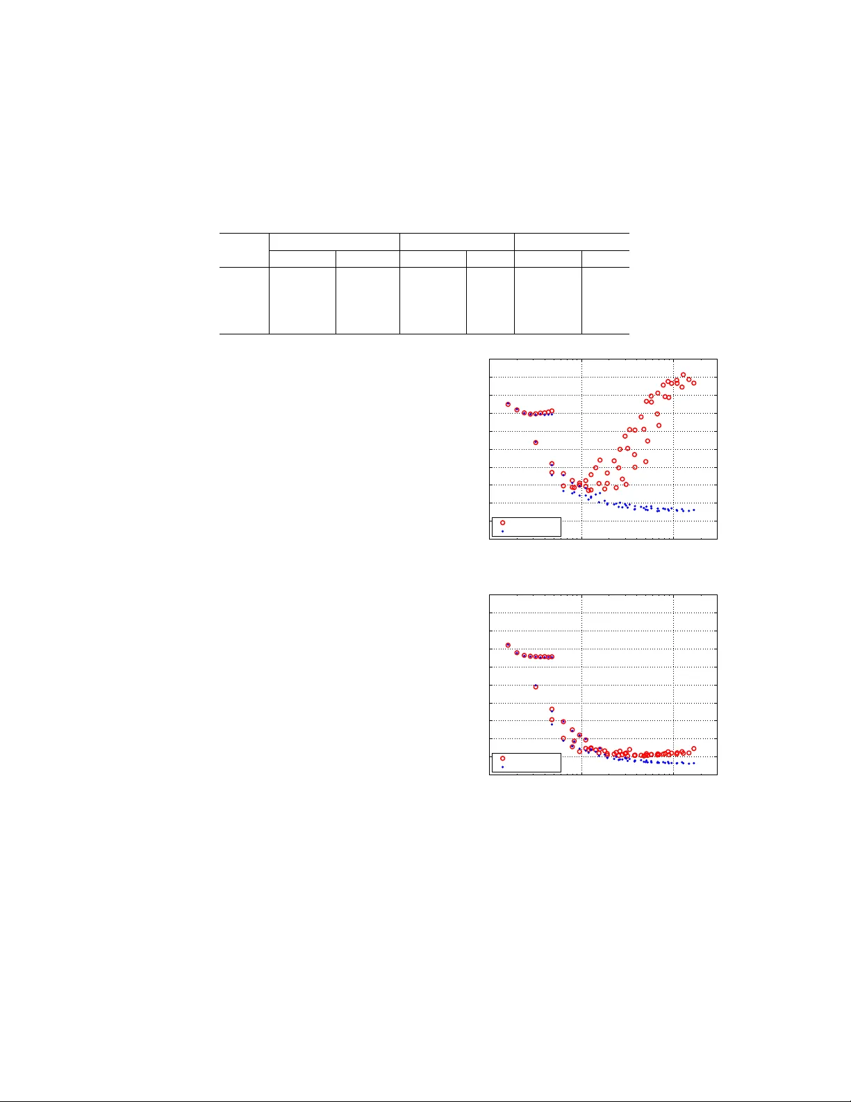
Scalable out-of-sample extension of graph em b eddings using deep neural net w orks Aren Jansen, Greg Sell, Vince Lyzinski Human Language T ec hnology Center of Excellence June 15, 2016 Abstract Sev eral p opular graph embedding techniques for rep- resen tation learning and dimensionalit y reduction rely on p erforming computationally expensive eigen- decomp ositions to derive a nonlinear transformation of the input data space. The resulting eigen vectors enco de the embedding co ordinates for the training samples only , and so the embedding of nov el data samples requires further costly computation. In this pap er, w e presen t a metho d for the out-of-sample ex- tension of graph embeddings using deep neural net- w orks (DNN) to parametrically approximate these nonlinear maps. Compared with traditional nonpara- metric out-of-sample extension metho ds, we demon- strate that the DNNs c an generalize with equal or b etter fidelit y and require orders of magnitude less computation at test time. Moreo ver, we find that unsup ervised pretraining of the DNNs improv es opti- mization for larger net work sizes, th us remo ving sen- sitivit y to mo del selection. 1 In tro duction Manifold learning is a p opular data analysis framew ork that attempts to recov er compact lo w-dimensional embeddings of high-dimensional datasets. Sev eral manifold learning algorithms— including ISOMAP (T enen baum et al., 2000), lo- cally linear em b edding (Ro weis and Saul, 2000, 2003), diffusion maps (Coifman and Lafon, 2006), and Laplacian eigenmaps (Belkin and Niyogi, 2003)— deriv e coordinate representations that enco de the lo cal neigh b orhoo d structure of an unlab eled data sample. These tec hniques ha ve found considerable success in a wide array of application domains, in- cluding computer vision (Elgammal and Lee, 2004; Murph y-Chutorian and T riv edi, 2009; He et al., 2005), sp eec h pro cessing (Jansen and Niyogi, 2006; Jansen et al., 2012; Jansen and Niyogi, 2013; T omar and Rose, 2013; Sahraeian and V an Comp ernolle, 2013; Mousazadeh and Cohen, 2013), and natural language pro cessing (Shi et al., 2007; Solk a et al., 2008). In (Y an et al., 2007), it w as sho wn that these algorithms are all members of a more general graph em b edding framew ork, in whic h the transformations are deriv ed via a generalized eigendecomp osition of the graph Laplacian matrix op erator for algorithm- sp ecific graph construction metho dologies. In their basic form, these graph em b edding tech- niques only provide transformations of the training samples used to construct the graph. Thus, even if a large training set is used, computing the output of the estimated map for a nov el test sample is not p ossible. T o address this shortcoming, a nonpara- metric out-of-sample extension technique based on Nystr¨ om sampling was dev elop ed that leverages the input and target representation pairs for eac h train- ing sample to approximate what the map would ha ve generated for an arbitrary test p oint (Bengio et al., 2004; Kumar et al., 2012). While generally effective, the Nystr¨ om extension is a k ernel-based method with time complexit y that scales linearly with the num- b er of training samples. This increase in computa- 1 tional cost is esp ecially problematic b ecause manifold metho ds are most effectiv e when provided the benefit of large training sets for representation learning. It w ould be highly b eneficial to remov e this trade-off b e- t ween represen tation qualit y and extension feasibilit y with a more efficiently scaleable metho d for out-of- sample extension. Neural netw orks hav e long b een known to be a p o w erful learning framework for classification and regression, capable of distilling large training se ts in to efficien tly ev aluated parametric mo dels, and thus are a natural choice for mo deling manifold em b ed- dings. In their seminal pap er, Hornik et al. (Hornik et al., 1989) prov ed that feedforward neural net- w orks can appro ximate a virtually arbitrary deter- ministic map b et ween high-dimensional spaces, indi- cating that they would also be ideally suited for our out-of-sample extension problem. How ever, there are t wo cav eats for the use of neural net works as univer- sal approximators: (i) there m ust b e sufficien t hid- den units (i.e. sufficien t mo del parameters), which in turn require additional data sam ples for training without ov erfitting; and (ii) the non-con vexit y of the ob jective function grows with the n umber of mo del parameters, making the searc h for reliable global so- lutions increasingly difficult. With these considerations in mind, w e explore the application of recent adv ances in deep neural netw ork (DNN) training metho dology to the out-of-sample ex- tension problem. First, by stabilizing the Lanczos eigendecomp osition algorithm, we are able to pro- duce exact graph embeddings for training sets with millions of data samples. This permits an extensive study with deep er arc hitectures than ha ve b een pre- viously considered for the task. Second, motiv ated by success in the supervised classification setting (Ben- gio, 2009; Bengio et al., 2007), w e consider unsup er- vised DNN pretraining pro cedures to improv e opti- mization as our larger training samples supp ort com- mensurate increases in model complexit y . In the work that follo ws, w e compare the p erfor- mance of our parametric DNN approach against a Nystr¨ om sampling baseline, b oth in terms of approx- imation fidelity and test runtime. W e find DNNs to match or outperform the approximation fidelity of the Nystr¨ om metho d for all training sample sizes. F urthermore, since the DNN approach is parametric, its test-time complexity for fixed netw ork size is con- stan t in the training sample size, producing orders-of- magnitude speedup ov er Nystr¨ om sampling for larger training sizes. The remainder of this paper is orga- nized as follo ws. W e b egin with an o v erview of prior w ork in out-of-sample extension for graph embed- dings. W e then describ e the strategy for stabilizing eigendecomp ositions for large training sets, follo wed b y a description of the pro cess for training our DNN out-of-sample extension to appro ximate the embed- ding for unseen data. Finally , w e analyze the recon- struction accuracy and computation sp eed of b oth the Nystr¨ om baseline and the DNN approach. 2 Prior W ork The most p opular methods for extending graph em- b eddings to unseen data ha ve b een based on Nystr¨ om sampling (Bengio et al., 2004; Kumar et al., 2012), and th us they will serve as the baseline in our exp er- imen ts. This is a nonparametric, kernel-based tech- nique that appro ximates the embedding of eac h test sample b y computing a weigh ted in terp olation of the em b eddings for training samples that were nearb y in the original input space. F ormally (see (Bengio et al., 2004) for details), let X = { x 1 , . . . , x n } be the set of graph em b edding training samples, where eac h x i ∈ R d . Let L b e the symmetric, normalized graph Laplacian operator defined for the set X such that L = I − D − 1 / 2 AD − 1 / 2 , where A i,j = K ( x i , x j ) for some p ositiv e semidefinite k ernel function K that m ust b e sp ecialized for each specific graph embed- ding algorithm; and D is the diagonal matrix defined via D i,i = P j A i,j . Let the spectral decomposition of the normalized Laplacian b e denoted as L = U Σ U T , where the diagonal entries of Σ are non-increasing. The d 0 -dimensional embedding of X is then provided b y the first d 0 columns of U , which we shall denote as U d 0 . Stated simply , the embedding of x i is giv en b y the i -th ro w of U d 0 . T o em b ed an out-of-sample data p oin t x ∈ R d via the Nystr¨ om extension, the p -th dimension of the ex- 2 tension y p ( x ) is given b y y p ( x ) = 1 λ p n X i =1 v pi K ( x, x i ) . (1) W e see that the complexity of this extension is lin- ear in the size of the training set. In practice, ap- pro ximate nearest neighbor tec hniques can b e used to sp eed this up with minimal loss in fidelit y (the im- plemen tation w e b enc hmark uses k-d tree for this pur- p ose), but the algorithmic complexit y still increases with training size. Finally , note that a nearly equiv a- len t form ulation based on repro ducing Kernel Hilb ert space theory was presented in (Belkin et al., 2006), where the k ernelization was introduced into the ob- jectiv e function before the eigendecomp osition is p er- formed. This formulation has the same scalabilit y limitations as the Nystr¨ om extension. These compu- tational difficulties motiv ate our exploration of DNNs to model em b eddings for out-of-sample extension. T raditional neural netw orks ha ve also b een consid- ered for out-of-sample extension in the past in tw o limited studies in volving small datasets and mo del arc hitectures (Gong et al., 2006; Chin et al., 2007). The idea was in tro duced in (Gong et al., 2006), but the study failed to include a meaningful quantitativ e ev aluation. The exp erimen ts in (Chin et al., 2007), whic h predated the adv ent of recen t deep learning training methodologies, found neural netw orks to b e one of the worst p erforming metho ds. Ho wev er, with a similar motive of computational efficiency , (Gregor and LeCun, 2010) explored the use of DNNs for ap- pro ximating exp ensiv e sparse coding transformations and produced more comp elling results. 3 A Scalable Out-of-Sample Extension A truly scalable out-of-sample extension must si- m ultaneously consume a large amoun t of training data for detailed mo deling and pro vide a test-time complexit y that do es not strongly depend on that training set size. The nonparametric nature of the Nystr¨ om metho d leads to a linear dep endence on the training set size (logarithmic if kernel appro ximations are implemen ted) and thus can get b ogged down as w e feed more data to the graph embedding train- ing. W e b egin this section with a simple trick for the eigendecomp osition of large graph Laplacians, whic h p ermits larger training sets and motiv ates the need for more computationally efficient extension meth- o ds. This is follow ed b y a presentation of the deep neural netw ork arc hitecture w e propose to efficiently extend the embedding to arbitrary test p oin ts. 3.1 Stabilizing the Eigendecomp osi- tion In (Golub and V an Loan, 2012), it is suggested that the stabilit y of the Lanczos eigendecomp osition al- gorithm can b e greatly increased (and memory re- quiremen ts consequently reduced) b y reformulating the eigenproblem to reco ver the largest eigenv alues. W e can exploit this b y observing that if v is an eigen- v ector of L with eigenv alue λ , then v is also an eigen- v ector of e L = I − L with eigen v alue 1 − λ (which is guaranteed to b e less than or equal to 1). Th us, with this small redefinition of the eigenproblem, w e can recov er the same eigenv ectors by considering the largest eigenv alue criterion. Note that when using the ARP ACK implementation, a similar effect can also b e accomplished by searc hing for the smallest algebr aic eigen v alues of L directly . While this tric k is by no means a fundamen tal theoretical inno v ation on our part, its effects ha ve pro ven dramatic. Our past efforts to solve for the smallest magnitude eigenv alues of the graph Lapla- cian exceeded our hardware memory limits when our graphs reached the order of 100,000 no des and 1 mil- lion edges. Emplo ying this simple tric k, we ha ve now succeeded in pro cessing graphs with order 100 mil- lion no des and order 10 billion edges on conv entional hardw are, stably solving for the top 100 eigenv ectors in a few days using 32 cores and 0.5 TB of RAM. This problem size even exceeds what was rep orted using appro ximate singular v alue decomp osition solvers in the past (T alw alk ar et al., 2008). F or the 1.5 million no de graphs we consider in our experiments describ ed b elo w, this method w as more than adequate for our (offline) em bedding training needs. 3 3.2 Deep Neural Net work Metho dol- ogy Solving the eigen v alue problem pro duces a d 0 - dimensional (exact) em b edding z i ∈ R d 0 for each x i ∈ X . Rather than viewing new data points as out- of-sample p oin ts whose mapping is estimated with in- terp olation, we instead seek to estimate the mapping (from x to z ) itself. T o this end, w e now consider feedforw ard neural architectures with N hidden la y- ers, eac h con taining M hidden units. The l -th hid- den lay er nonlinearly maps the output of the previous la yer h l − 1 to a new hidden representation h l ∈ R M according to h l = σ ( W l h l − 1 + b l ) , (2) where each W l is a parameter matrix, b l is a bias col- umn vector, and σ is the activ ation function (which w e set to tanh in our exp erimen ts). The input h 0 to the first la yer is a point x in our input space R d , while W 1 ∈ R M × d , W l ∈ R M × M for l ∈ { 2 , . . . , N } , and b l ∈ R M for l ∈ { 1 , . . . , N } . The output h l of these N hidden la yers are finally transformed into a corresp onding p oin t y ( x ) ∈ R d 0 according to y ( x ) = W N +1 h N + b N +1 , (3) where W N +1 ∈ R d 0 × M and b N +1 ∈ R d 0 are the de- co ding weigh t matrix and bias column vector, respec- tiv ely . The training ob jective is to solv e for param- eters Θ ∗ = { W ∗ 1 , . . . , W ∗ N +1 , b ∗ 1 , . . . , b ∗ N +1 } that mini- mize mean squared error betw een the exact and pre- dicted em bedding pairs: Θ ∗ = arg min Θ 1 n n X i =1 k z i − y ( x i ) k 2 . (4) This is generally accomplished with backpropagation and stochastic gradient descen t optimization. It is critical that the training pro cedure safeguards against ov erfitting to the training sample, esp ecially as deep er architectures are required in order to ap- pro ximate the detailed graph embeddings w e wish to extend. Our training procedure, which w as also em- plo yed in (Kamp er et al., 2015) for a different applica- tion, has tw o steps: (i) unsup ervised stack ed auto en- co der pretraining that uses X only , and (ii) super- vised fine-tuning using the ( x i , z i ) pairs as training inputs and targets. 3.2.1 Unsup ervised Pretraining When the input and output targets are the same, our deep netw ork arc hitecture reduces to a stack ed au- to encoder (SAE) with N enco ding lay ers and one de- co ding lay er. Th us, to initialize model parameters of the DNN to approximately reco ver the iden tity map- ping, we consider the unsup ervised SAE pretraining pro cedure (Bengio, 2009; Bengio et al., 2007). Here, w e in tro duce one hidden lay er at a time, p erform- ing several ep ochs of sto c hastic gradient descent to minimize mean squared error b et ween our training samples and themselv es at each intermediate net work depth. As we add each new lay er, w e discard the lin- ear deco ding w eights from the previous optimization, use the previous hidden represen tation as input to the new hidden lay er, and reoptimize all la yer pa- rameters. Early stopping is used to prev ent exact reco very of the identit y map for eac h la yer. 3.2.2 Sup ervised Fine-T uning Using the ab o v e la yer-wise pretraining pro cedure, we no w ha ve initialized all parameters in the net work. It only remains to p erform several ep ochs of sto c has- tic gradient descen t to reoptimize netw ork param- eters to minimize mean squared error b etw een the exact and predicted em b edding pairs according to Equation (4). After this training is complete, the DNN-based out-of-sample extension y ( x ) for an arbi- trary p oin t x ∈ R d can b e efficiently computed using the standard neural netw ork forw ard pass defined by Equation (3). This amounts to N + 1 matrix-v ector m ultiplies and vector additions, plus an ev aluation of σ for eac h hidden unit. F or a fixed netw ork architec- ture, this computation is constant in the n umber of training samples. 4 Exp erimen ts W e c ho ose sp eec h as the application domain for our scalabilit y study for tw o reasons: (i) a single hour 4 Squared Bandwidth, σ 2 Number of Neighbors, k 0.005 0.025 0.05 0.25 0.5 2.5 1 5 10 25 50 100 500 0.2 0.3 0.4 0.5 0.6 (a) Nystr¨ om, n = 1 , 000 Squared Bandwidth, σ 2 Number of Neighbors, k 0.005 0.025 0.05 0.25 0.5 2.5 1 5 10 25 50 100 500 0.2 0.3 0.4 0.5 0.6 (b) Nystr¨ om, n = 10 , 000 Squared Bandwidth, σ 2 Number of Neighbors, k 0.005 0.025 0.05 0.25 0.5 2.5 1 5 10 25 50 100 500 0.2 0.3 0.4 0.5 0.6 (c) Nystr¨ om, n = 100 , 000 Squared Bandwidth, σ 2 Number of Neighbors, k 0.005 0.025 0.05 0.25 0.5 2.5 1 5 10 25 50 100 500 0.2 0.3 0.4 0.5 0.6 (d) Nystr¨ om, n = 1 , 100 , 000 0 0.2 0.4 0.6 0.8 1 0 0.1 0.2 0.3 0.4 0.5 0.6 0.7 0.8 0.9 1 0.2 0.25 0.3 0.35 0.4 0.45 0.5 0.55 0.6 NRMSE Layer Size, M Number of Layers, N 20 40 60 80 100 120 140 1 2 3 4 5 6 7 8 9 0.2 0.3 0.4 0.5 0.6 (e) DNN, n = 1 , 000 Layer Size, M Number of Layers, N 20 40 60 80 100 120 140 1 2 3 4 5 6 7 8 9 0.2 0.3 0.4 0.5 0.6 (f ) DNN, n = 10 , 000 Layer Size, M Number of Layers, N 20 40 60 80 100 120 140 1 2 3 4 5 6 7 8 9 0.2 0.3 0.4 0.5 0.6 (g) DNN, n = 100 , 000 Layer Size, M Number of Layers, N 20 40 60 80 100 120 140 1 2 3 4 5 6 7 8 9 0.2 0.3 0.4 0.5 0.6 (h) DNN, n = 1 , 100 , 000 Figure 1: Heat maps showing the NRMSE v alues for all Nystr¨ om (a-d) and DNN (e-h) hyperparameter settings, for each of the four training set sizes. The same color scale is used for all images. of audio recordings t ypically pro duce 360,000 high- dimensional data samples kno wn as frames, and so large datasets are readily a v ailable; and (ii) mani- fold learning techniques hav e b een shown to learn represen tations effective for keyw ord disco very and searc h (Jansen et al., 2012; Jansen and Niy ogi, 2013; Jansen et al., 2013). W e use the TIMIT corpus for ev aluation, given the past success of manifold em- b eddings for sp eec h recognition on that data (Jansen et al., 2012). It consists of o ver 4 hours of prompted American English sp eec h recordings, and is split into a training set consisting of roughly 1.1 million data samples ( ∼ 3 hours) and a test set of roughly 400,000 data samples ( ∼ 1 hour). There is no sp eak er o verlap b et w een the tw o sets. 4.1 Ev aluation Metho dology Our goal is to measure the approximation fidelity of the out-of-sample extension of the test set against a reference embedding that is indep endent of the exten- sion metho d. Thus, our strategy is to p erform an ex- act graph em b edding of the entire corpus (train+test) using the method describ ed in Section 3.1; we call these the r efer enc e emb e ddings . W e define each out- of-sample extension using input frames and corre- sp onding reference em b eddings from the training set. This allows us to use reference embeddings for the training set to approximate embeddings for the test set for comparison against the true reference em b ed- dings of the test set. W e measure appro ximation fi- delit y in terms of normalized ro ot mean squared er- ror (NRMSE) b et ween the predicted and reference test em b eddings; here, the normalization constan t is tak en to b e the ro ot mean squared error b et ween the test set reference em b eddings and a random p erm u- tation of those same samples. Th us, a p erfect out- of-sample extension will hav e NRMSE of 0, while a extension that is a random mapping with the same empirical output distribution will hav e NRMSE of 1. In addition to defining the extensions with the entire training set (1.1 M samples), we also consider the 5 utilit y of random subsets of sizes 1,000, 10,000, and 100,000. How ever, we use the same reference embed- dings for all experiments. Our input features are 40-dimensional, homomor- phically smo othed, mel-scale, log p o w er sp ectrograms (40 equally spaced mel bands from 0-8 kHz), sampled ev ery 10 ms using a 25 ms Hamming windo w. W e construct the graph Laplacian using a symmetrized 10-nearest neighbor adjacency graph with cosine dis- tance as the metric and binary edge w eights. This amoun ts to a Laplacian eigenmaps sp ecialization of the graph em b edding framew ork. Finally , w e keep the 40 eigenv ectors with the largest eigenv alues to pro duce a graph em b edding with the same dimen- sion as the input space. While our presen t fo cus is on out-of-sample extension fidelity , it is relev an t to note that the reference embeddings matc h the b est down- stream performance reported in (Jansen and Niy ogi, 2013), whic h used an iden tical embedding strategy . F or the baseline Nystr¨ om metho d, we compute Equation (1) using a nearest neighbor approxima- tion to a radial basis function (RBF) k ernel. This appro ximation is facilitated b y prepro cessing the training samples in to a k-d tree data structure (as implemented in scikit-learn ) for efficient re- triev al of near-neigh b or sets. Note that we tried matc hing the Nystr¨ om kernel to that used in the graph construction (i.e., using binary weigh ts) as prescrib ed by (Bengio et al., 2004), but it per- formed substantially worse than introducing RBF w eights. W e consider k ernel squared-bandwidths σ 2 ∈ { 0 . 005 , 0 . 025 , 0 . 05 , 0 . 25 , 0 . 5 , 2 . 5 } and n umber of neigh b ors k ∈ { 1 , 5 , 10 , 25 , 50 , 100 , 500 } . F or our DNN metho d, w e consider L ∈ { 1 , 2 , . . . , 9 } hidden lay ers, and for each depth w e ev aluate la yer sizes of M ∈ { 20 , 40 , 60 , 80 , 100 , 120 , 140 } hidden units. F or pretraining, we use the entire train- ing set and optimize each lay er for 15 ep ochs of sto c hastic gradient descen t. F ollo wing the prescrip- tion in (Kamp er et al., 2015), w e use a learning rate of 2 . 5 × 10 − 4 and minibatches of 256 samples. F or sup er- vised fine-tuning, we increase the num b er of ep ochs for the smaller training sets suc h that the total n um- b er of examples processed is roughly fixed (5 epo c hs for the full train set of 1.1 million samples, 50 ep o c hs for 100,000 samples, etc) to ensure adequate conv er- gence. Also following (Kamp er et al., 2015), for fine- tuning w e use a learning rate of 4 × 10 − 3 , but found a smaller minibatch of size 50 improv ed conv ergence. W e use the Pylearn2 to olkit (Go odfellow et al., 2013) for all DNN experiments. 4.2 Hyp erparameter Sensitivity First, w e consider the NRMSE p erformance as w e v ary the amoun t of training samples used by the out- of-sample extension. W e drew random subsets of the 1.1 million sample training set of sizes 1000, 10,000, and 100,000. Eac h of these subsets was used for com- putation of Equation (1) in the Nystr¨ om metho d and for sup ervised fine-tuning in the case of the DNN metho d. T able 1 lists for eac h training subset size the NRMSE and test runtime for (i) Nystr¨ om using the optimal set of hyperparameters, (ii) a smaller DNN with 2 la yers of 60 units eac h, (iii) a larger DNN with 5 la yers of 140 units. W e see that the larger DNN matches or outp erforms the Nystr¨ om metho d for all training set sizes, demonstrating the pow er of deep learning for accurately appro ximating complex nonlinear functions. While the small DNN matches Nystr¨ om for the 2 smaller training sets, it do es not ha ve sufficient parameters to k eep pace as more train- ing data b ecomes av ailable. These results emphasize the imp ortance of eac h metho d’s sensitivity to the c hoice of hyparameters that sp ecify the complexity of the out-of-sample ex- tension function. This is esp ecially true for fully unsup ervised representation learning settings, where cross-v alidation may not b e p ossible. T o explore this consideration, for the Nystr¨ om metho d, we v ary the n umber of (approximate) nearest neigh b ors that con- tribute to each test sample, as well as the kernel band- width. F or the prop osed DNN metho d we v ary b oth the n umber of la yers ( N ) and the num b er of hidden units per la yer ( M ). Figure 1 shows heatmaps indicating the NRMSE for all hyperparameters considered for the tw o meth- o ds for the four training set sizes. F or the Nystr¨ om metho d, performance is relativ ely stable across the range of k ernel bandwidths, but it is more sensitive to the num b er of neighbors used in the computation. Moreo ver, the optimal num b er of neighbors increases 6 T able 1: T est set NRMSE and runtime (in seconds, av eraged o ver sev eral trials) for Nystr¨ om with optimal h yp erparameters, a small DNN ( N = 2 , M = 60), and a large DNN ( N = 5 , M = 140). T rain Nystr¨ om (optimal) Small DNN Large DNN Size NRMSE Time NRMSE Time NRMSE Time 1k 0.36 25 0.33 5.4 0.28 33 10k 0.29 240 0.29 5.4 0.24 33 100k 0.25 2,200 0.29 5.4 0.23 33 1.1M 0.24 12,000 0.29 5.4 0.23 33 as more training data is av ailable, necessitating some amoun t of parameter tuning to achiev e optimal ap- pro ximation. The DNN approach reac hes near-optimal p erfor- mance for all training set sizes provided w e include at least 4 lay ers with at least t wice as many units than the input dimension. Critically , there is no p er- formance p enalt y for o vershooting the netw ork size (other than increased forw ardpass run time, as w e dis- cuss b elo w). This suggests the DNN extension would require less tuning than Nystr¨ om metho d to ac hieve optimal appro ximation in new applications. 4.3 The Effect of Pretraining In t ypical machine learning scenarios, increasing the n umber of model parameters for a fixed training set size opens the metho d up to o verfitting and po or gen- eralization. The trends for the DNN metho ds in Fig- ure 1 defy this con ven tional wisdom, with no loss in appro ximation fidelity for any training corpus size as w e mov e to deep er and wider netw ork architectures. Indeed, the unsup ervised pretraining is resp onsible for regularizing the parameter estimates, preven ting o verspecialization to even the smallest training set considered. This can b e seen most clearly in the scatterplots in Figure 2, where each dot represen ts a single mo del arc hitecture. As the total num b er of parameters increases, the test NRMSE of the pre- trained models decays roughly monotonically . The same arc hitectures without pretraining track simi- larly for smaller model sizes, but, due to o verfitting, the test p erformance degrades as more parameters are made a v ailable. This b eha vior is esp ecially clear in the case of limited training examples, though w e 10 3 10 4 10 5 0.2 0.25 0.3 0.35 0.4 0.45 0.5 0.55 0.6 0.65 0.7 Number of DNN Parameters NRMSE w/o Pretraining w/ Pretraining (a) 1,000 T raining Pairs 10 3 10 4 10 5 0.2 0.25 0.3 0.35 0.4 0.45 0.5 0.55 0.6 0.65 0.7 Number of DNN Parameters NRMSE w/o Pretraining w/ Pretraining (b) 1,100,000 T raining Pairs Figure 2: Approximation fidelit y vs. num b er of DNN parameters for (a) 1,000 and (b) 1.1 million training set sizes, both with and without unsupervised pre- training. 7 see the beginnings of the same effect for the largest arc hitectures even in the presence of the full training set. 4.4 T est Run times Finally , we consider the computational efficiency of applying the tw o out-of-sample extension metho ds to a test corpus. T able 1 lists the NRMSE v alues and corresp onding test times in seconds (i.e., the time tak en to extend the embedding to the entire 400,000 sample test set) for the Nystr¨ om method with optimal hyperparameters and tw o DNN archi- tectures. As exp ected, the run times for the nonpara- metric Nystr¨ om metho d increase as the training sam- ple gets bigger, since nearest neighbor retriev al re- mains exp ensiv e even when using the k-d tree data structure. Mean while, the DNN run times are virtu- ally constan t for a fixed n umber of parameters. The small DNN can consume the full training set and pro- duce extensions o ver 4 times faster than the Nystr¨ om metho d with the smallest training set, while simul- taneously reducing NRMSE b y 20% relative. More- o ver, the b est DNN roughly matches the approxima- tion fidelity of the b est Nystr¨ om NRMSE, and the DNN accomplishes it ∼ 350 times faster. F or all train- ing sizes tested, DNN extensions can provide signfi- can t sp eedup without any sacrifices in fidelity , and, in man y cases, impro ve b oth speed and fidelity . F or speech pro cessing applications, where in terac- tivit y is often critical, ev en our largest net works can pro cess test samples faster than real-time. Moreov er, with the large DNN consisting of 5 lay ers of 140 hid- den units, optimal NRMSE is achiev ed at sp eeds 120 times faster than real-time using a single pro cessor. This is comparable to the extraction sp eed of tra- ditional acoustic front-ends in state-of-the-art imple- men tations (P ov ey et al., 2011). 5 Conclusion In this work, we used mo dern deep learning metho d- ologies to p erform out-of-sample extensions of graph em b eddings. Compared with the standard Nystr¨ om sampling-based out-of-sample extension, the DNNs appro ximate the embeddings with higher fidelit y and are substan tially more computationally efficient. Us- ing unsupervised pretraining for parameter initializa- tion impro ves DNN generalization, making our DNN approac h highly stable across a wide v ariety of h y- p erparameter settings. These results supp ort deep neural netw orks with unsupervised pretraining as an ideal c hoice for out-of-sample extensions of learned manifold represen tations. Ac kno wledgmen t The authors w ould lik e to thank Herman Kamper of the Universit y of Edinburgh for pro viding his corre- sp ondence auto encoder to ols, on which we based our neural net w ork implemen tation. References Belkin, M., Niyogi, P ., 2003. Laplacian Eigenmaps for Dimensionalit y Reduction and Data Represen- ation. Neural Computation 16, 1373–1396. Belkin, M., Niy ogi, P ., Sindhw ani, V., 2006. Manifold regularization: A geometric framework for learning from examples. Journal of Machine Learning Re- searc h 7, 2399–2434. Bengio, Y., 2009. Learning deep architectures for AI. F oundations and T rends in Machine Learning 2, 1–127. Bengio, Y., Lamblin, P ., Popovici, D., Laro c helle, H., et al., 2007. Greedy la yer-wise training of deep net- w orks. Adv ances in Neural Information Pro cessing Systems 19, 153. Bengio, Y., Paiemen t, J.F., Vincent, P ., Delalleau, O., Le Roux, N., Ouimet, M., 2004. Out-of-sample extensions for LLE, Isomap, MDS, Eigenmaps, and sp ectral clustering. Adv ances in neural information pro cessing systems 16, 177–184. Chin, T.J., W ang, L., Schindler, K., Suter, D., 2007. Extrap olating learned manifolds for human activ- it y recognition, in: Image Pro cessing, 2007. ICIP 8 2007. IEEE In ternational Conference on, IEEE. pp. I–381. Coifman, R.R., Lafon, S., 2006. Diffusion Maps. Ap- plied and Computational Harmonic Analysis 21, 5–30. Elgammal, A., Lee, C.S., 2004. Inferring 3D b o dy p ose from silhouettes using activit y manifold learn- ing, in: Computer Vision and P attern Recognition, 2004. CVPR 2004. Pro ceedings of the 2004 IEEE Computer Society Conference on, IEEE. pp. I I– 681. Golub, G.H., V an Loan, C.F., 2012. Matrix compu- tations. v olume 3. JHU Press. Gong, H., Pan, C., Y ang, Q., Lu, H., Ma, S., 2006. Neural netw ork mo deling of sp ectral embedding., in: BMVC, pp. 227–236. Go odfellow, I.J., W arde-F arley , D., Lamblin, P ., Du- moulin, V., Mirza, M., Pascan u, R., Bergstra, J., Bastien, F., Bengio, Y., 2013. Pylearn2: a ma- c hine learning researc h library . arXiv preprint arXiv:1308.4214 . Gregor, K., LeCun, Y., 2010. Learning fast appro x- imations of sparse co ding, in: Proceedings of the 27th In ternational Conference on Machine Learn- ing (ICML-10), pp. 399–406. He, X., Y an, S., Hu, Y., Niy ogi, P ., Zhang, H.J., 2005. F ace recognition using Laplacianfaces. Pattern Analysis and Mac hine Intelligence, IEEE T ransac- tions on 27, 328–340. Hornik, K., Stinc hcombe, M., White, H., 1989. Mul- tila yer feedforward netw orks are universal approx- imators. Neural net works 2, 359–366. Jansen, A., Dup oux, E., Goldwater, S., Johnson, M., Kh udanpur, S., Churc h, K., F eldman, N., Herman- sky , H., Metze, F., Rose, R., et al., 2013. A sum- mary of the 2012 JHU CLSP workshop on zero re- source speech tec hnologies and mo dels of early lan- guage acquisition, in: Acoustics, Speech and Sig- nal Pro cessing (ICASSP), 2013 IEEE International Conference on, IEEE. Jansen, A., Niy ogi, P ., 2006. Intrinsic F ourier analysis on the manifold of speech sounds, in: Pro ceedings of ICASSP . Jansen, A., Niyogi, P ., 2013. Intrinsic spectral anal- ysis. Signal Processing, IEEE T ransactions on 61, 1698–1710. Jansen, A., Thomas, S., Hermansky , H., 2012. In- trinsic sp ectral analysis for zero and high resource sp eec h recognition, in: In tersp eec h. Kamp er, H., Elsner, M., Jansen, A., Goldwater, S., 2015. Unsup ervised neural netw ork based feature extraction using w eak top-down constraints, in: Pro ceedings of ICASSP . Kumar, S., Mohri, M., T alw alk ar, A., 2012. Sampling metho ds for the Nystr¨ om metho d. The Journal of Mac hine Learning Research 13, 981–1006. Mousazadeh, S., Cohen, I., 2013. Voice Activit y De- tection in Presence of T ransient Noise Using Spec- tral Clustering. IEEE T ransactions on Acoustics, Sp eec h, and Language Processing 21, 1261–71. Murph y-Chutorian, E., T rivedi, M.M., 2009. Head p ose estimation in computer vision: A survey . P attern Analysis and Machine In telligence, IEEE T ransactions on 31, 607–626. P ov ey , D., Ghoshal, A., Boulianne, G., Burget, L., Glem b ek, O., Go el, N., Hannemann, M., Motl ´ ıˇ cek, P ., Qian, Y., Sc hw arz, P ., et al., 2011. The Kaldi sp eec h recognition to olkit, in: Proc. of the ASRU. Ro weis, S.T., Saul, L.K., 2000. Nonlinear dimension- alit y reduction by locally linear embedding. Science 290, 2323–2326. Ro weis, S.T., Saul, L.K., 2003. Think globally , fit lo cally: Unsup ervised learning of low dimensional manifolds. J. of Machine Learning Research 4, 119– 155. Sahraeian, R., V an Comp ernolle, D., 2013. A study of sup ervised intrinsic spectral analysis for timit phone classification, in: Automatic Sp eec h Recog- nition and Understanding (ASRU), 2013 IEEE W orkshop on, IEEE. pp. 256–260. 9 Shi, L., Zhang, J., Liu, E., He, P ., 2007. T ext classifi- cation based on nonlinear dimensionalit y reduction tec hniques and supp ort vector machines, in: Nat- ural Computation, 2007. ICNC 2007. Third Inter- national Conference on, IEEE. pp. 674–677. Solk a, J.L., et al., 2008. T ext data mining: theory and methods. Statistics Surveys 2, 94–112. T alw alk ar, A., Kumar, S., Ro wley , H., 2008. Large- scale manifold learning, in: Computer Vision and P attern Recognition, 2008. CVPR 2008. IEEE Conference on, IEEE. pp. 1–8. T enen baum, J.B., de Silv a, V., Langford, J.C., 2000. A global geometric framew ork for nonlinear dimen- sionalit y reduction. Science 290, 2319–2323. T omar, V.S., Rose, R.C., 2013. Efficien t manifold learning for sp eec h recognition using lo cality sensi- tiv e hashing, in: Acoustics, Sp eec h and Signal Pro- cessing (ICASSP), 2013 IEEE International Con- ference on, IEEE. pp. 6995–6999. Y an, S., Xu, D., Zhang, B., Zhang, H.J., Y ang, Q., Lin, S., 2007. Graph embedding and extensions: a general framework for dimensionality reduction. P attern Analysis and Machine In telligence, IEEE T ransactions on 29, 40–51. 10