Gaussian Processes for Music Audio Modelling and Content Analysis
Real music signals are highly variable, yet they have strong statistical structure. Prior information about the underlying physical mechanisms by which sounds are generated and rules by which complex sound structure is constructed (notes, chords, a c…
Authors: Pablo A. Alvarado, Dan Stowell
Gaussian Pro cesses for Music Audio Mo delling and Con ten t Analysis P ablo A. Alv arado, Dan Sto w ell Queen Mary Unive rsity of London June 13, 20 16 Abstract Real music signals are highly v ariable, yet th ey hav e strong statistical structure. Prior information about the underlying physical mec h anisms by whic h sounds a re generated and rules b y whic h complex sound struc- ture is constructed (notes, c hords, a co mp lete musical score), can b e nat- urally unified using Ba yesian mo delling tec hniques. Typically algorithms for Automatic Music T ranscription indep endently carry out individual tasks suc h as multiple-F0 detection a n d beat tracking. The chall enge remains to p erform j oint estimati on of all parameters. W e present a Ba- yesi an app roac h for mo delling m usic audio, and content analysis. The prop osed method ology b ased on Gaussian processes seeks joint estima- tion of m ultiple music concepts b y incorp orating into the k ernel prior information ab ou t non-stationary behaviour, dynamics, and rich spectral conten t present in the mod elled music signal. W e illustrate th e b enefits of th is approach via tw o t asks: pitc h estimation, and inferring missing segmen ts in a polyph onic audio recording. 1 In tro du ction In m usic informatio n research, the aim of audio con tent analysis is to estimate m usic al concepts which are present but hidden in the audio data [17]. With this purp ose, differ e n t signa l pro cessing techniques ar e applied to music signals for extracting us eful informa tio n and descriptors rela ted to the musical concepts. Here, musical concepts refers to parameters related to written music, such a s pitc h, melo dy , c ho rds, onse t, b eat, temp o a nd rh ythm. Then, p erhaps the most ge ne r al applicatio n is one which in volves the prediction o f sev era l musical dimensions, that of recov er ing the score of a music track given only the audio signal [10]. This is known as automatic music t r anscription (AMT) [5 ]. AMT refer s to extraction o f a human readable and interpretable descr iption from a recording of a music pe rformance. W e r efer to po lyphonic AMT in cases where mor e than a single m usical pit ch plays at a given time insta nt . The general tas k of interest is to infer automa tically a musical notatio n, such as the traditional western m usic notation, listing the pitch v alues of notes, co rresp ond- ing timestamps a nd o ther expressive infor mation in a given a udio signal of a per formance [7]. T ranscribing p olyphonic music is a nontrivial task, esp ecially in its more unco nstrained for m when the task is per formed on an ar bitrary 1 acoustical input, and music transcription remains a very challenging pro blem [4]. Real music signals are highly v a riable, but nevertheless they hav e strong sta- tistical structure. Prior information ab out the underlying structur e s, such a s knowledge of the physical mec hanisms by which sounds are generated, a nd knowledge ab out the rules by whic h complex sound s tructure is compiled (notes, chords, a co mplete musical score), can b e na turally unified using Bay es ia n hier- archical mo de lling tec hniques. This allo ws the formulation of highly structur ed probabilistic models [7]. On the other hand, typically , a lgorithms for AMT are developed indep endently to car ry out indiv idua l ta sks such as multiple-F0 de- tection, b ea t tra cking and instrumen t recognition. The challenge remains to combine these algorithms, to p er form join t estimation of all parameters [5 ]. W e prese nt the design, implemen tation, and r esults of exp eriments of an al- ternative Bay esia n approach for audio conten t a nalysis on monophonic, and po lyphonic m usic signals with the pos sibility of b eing used for AMT. W e use Gaussian pro cess (GP) mo dels for jointly uncovering m usic concepts from au- dio, b y intro ducing a direct co nnec tio n betw een the music concepts and the mo del hyper-pa r ameters. The prop os ed metho do logy allows to incorp or ate in the mo del prior information ab out ph ysica l or mechanistic b ehaviour, no ns tatio- narity , time dynamics (lo cal p erio dicity , and non constant amplitude env elo p e), sp ectral harmonic co nt ent, and m usica l structure, laten t in the mo delled mu- sic signal. Spec ific a lly in the context of music infor matics, w e present kernels that embo dy a proba bilistic mo del of music notes a s time-limited harmonic sig- nals with onsets and o ffsets. A comparison with related w ork is provided in section 4.3. W e illustra te the be nefits of this approach via tw o tasks : pitch estimation, a nd inferring missing segmen ts in a p oly pho nic audio reco rding. As part of w o rking tow ards a high-r esolution AMT system, out metho d corr ectly estimates polyphonic pitch while per fo rming these s ample-level tasks. 2 Gaussian pro cess regression for m usic signals Gaussian pro cess -based machine learning is a p ow er ful Bayesian paradigm for nonparametric nonlinear r egress ion and classifica tion [14]. Gaussian Pro cess es (GPs) can be defined as distr ibutions o ver functions s uch that any finite num b er of function ev aluations f = [ f ( t 1 ) , · · · , f ( t N )], have a jointly normal distribution [12]. A GP is co mpletely sp ecified by its mean function µ ( t ) = E [ f ( t )] (in this work it is assumed to be µ ( t ) = 0 ), and its kernel or cov aria nce function k ( t, t ′ ) = E [( f ( t ) − µ ( t ))( f ( t ′ ) − µ ( t ′ ))] , (1) where k ( t, t ′ ) has hyper -parameter s θ . W e write the Gauss ia n process as f ( t ) ∼ G P ( µ ( t ) , k ( t, t ′ )) . (2) The r e g ressio n problem co ncerns the pr ediction o f a contin uous quantit y [12], here a function f ( t ), given a data set D = { ( t i , y i ) } N i =1 , where y i are a ssumed as noisy measurements of f ( t ) at typically reg ularly-spa ced time instants t i (though GP reg ression framework allows for irregula r sampling or missing data), i.e. y i = f ( t i ) + ǫ i , where ǫ i ∼ N (0 , σ 2 noise ). In GP reg ression for mo no channel audio signals, instead of estimating para meters η of fixed-form functions f ( t, η ) : R 7→ 2 R where the time input v a riable t ∈ R , we mo del the whole function f ( t ) as a GP . That is , instead of putting a prior ov er the function par ameters η , we introduce a prior o ver the function f ( t ) itself [1 6]. Lea rning in GP regression co rresp onds to co mputing the p o sterior distribution over the function f ( t ) conditioned on the observed da ta y = [ y 1 , · · · , y N ] ⊤ [15, 13]. The underlying idea in GP reg ression is that the cor relation function in tro- duces dep endences be t ween function f ( t ) v a lues at different inputs. Th us, the function v alues a t the obs erved p o int s give information also of the unobser ved po ints [14]. The structur e of the kernel (1) captures high-level pro p erties o f the unknown function f ( t ), which in turn deter mines how the mo del genera lizes or extr ap olates to new test time instant s [9]. This is quite useful b ecause we can in tr o duce prior knowledge ab out what we b elieve the pro prieties o f music signals a re, b y choos ing a pro pe r kernel that reflec ts those characteristics. In section 2.2 we s tudy in mo re detail the design of kernels. 2.1 Mo del definition Under a non-par a metric Bay esian regr ession approach using Gaussian pro cesses we a re in teres ted in calcula ting the p osterior dis tr ibution ov er a sto chastic func- tion ev aluated at test points t ∗ , that is , the joint distribution of the vector f observed only via n o isy measuremen ts y , then p ( f | y ) = p ( y | f ) × p ( f | θ ) p ( y ) , (3) where p ( y | f ) correspo nds to the lik eliho o d, p ( f | θ ) to the pr io r, θ are the model hyper-para meters (prior par ameters), p ( y ) is the evidence or marginal-likeliho o d, and p ( f | y ) is the p osterio r or conditional predictive distribution. W e describ e each of these f o ur expressions in the next sections. 2.1.1 Lik eli ho o d Assuming that conditioned on the f ( t i ) the signal observ ations y i are i.i.d. (independent and ident ica lly distributed), then the joint pro bability distribution of all the observ ations y follows a Gauss ia n distribution corr esp onding t o p ( y | f , σ 2 noise ) = N ( y | f , σ 2 noise I N ) , (4) where f i = f ( t i ) and I N is an identit y matrix of size N . 2.1.2 Prior Using the definition of GPs intro duced at the b eginning of this section, and knowing tha t we hav e a finite set of corr upted observ ations y , then the finite set o f GP function ev aluation v a lue s f follows a normal marginal distribution p ( f | θ ) conditioned on the hyper-pa r ameters θ , whose mean is zer o and who se cov aria nc e is defined by a Gram ma trix K f , this is p ( f | θ ) = N ( f | 0 , K f ) , (5) where the cov ariance matrix is calculated using (1), i.e. [ K f ] i,j = k ( t i , t j ) [6]. 3 2.1.3 Marginal-Lik el iho o d The mar ginal-likeliho o d (or evidence) p ( y ) mentioned b efor e in (3) is the in tegr al of the likeliho o d times the prior [12] p ( y ) = Z p ( y | f ) p ( f | θ )d f . (6 ) Since the likelihoo d p ( y | f ) and the prior p ( f | θ ) a r e multiv ariate Gaussian dis- tributions, w e can calculate directly the in teg ral in (6). Using the properties of the nor mal distribution [6] for marginal and conditional no rmal distributions, we obtain p ( y ) = N ( y | 0 , K y ) , (7) where the v a lues in the matrix K y = K f + σ 2 noise I dep end on the h yp er- parameters θ (w e have included σ 2 noise in the h yp er- parameters vector). The reason it is called the marginal likeliho o d, rather than just likelihoo d, is be- cause w e ha ve ma r ginalized out the laten t Gaussian v ector f [11]. 2.1.4 P osterior The computation of the p osterior distributio n o f the Gaussian pro cess condi- tioned on the set of mea surements y a nd estimation of the para meters θ of the cov aria nc e function of the pro ces s corres po nd to learning in this non-para metric mo del [14]. Using the pr op erties of Gaussian distribution [6, 12], the p osterior has the for m p ( f | y ) = N ( y | µ p os , K p os ) , (8) where the po sterior mean is µ p os = K f K − 1 y f , and the posterio r co v ariance matrix is K p os = K f − K ⊤ f K y K f . 2.2 Kernel design The cov a r iance function (1) used for computing the prior distributio n (5) al- lows us to in tro duce in the model a ll the knowledge and beliefs we ha ve ab o ut the prop er ties of the data. W e are trying to mo del music signals, a nd s o me of the broad prop erties o f audio signals are non-sta tio narity , rich sp ectral co nten t, dynamics (lo cally p erio dic, non constant amplitude en velop e), mechanistic be- haviour, and m usic structure. Therefore we seek co v aria nce f unctions that can describ e or r eflect these pr o p erties. One p ow erful technique for constructing ne w kernels is to build them out o f simpler kernels as building blo cks [19 , 6]. Two useful pr op erties w e ca n use to build v alid kernels ar e as follows: k ( t, t ′ ) = φ ( t ) k 1 ( t, t ′ ) φ ( t ′ ) , and k ( t, t ′ ) = k 1 ( t, t ′ ) + k 2 ( t, t ′ ) , wher e φ ( · ) is any function. Other pro p er ties can be found in [6]. W e use these prop erties for building non-statio na ry co v ariance functions. 2.2.1 Kernels for describi ng non-statio narit y T o construc t non-stationary kernels we com bine basic stationar y co v aria nce functions. W e use change-window s in order to be able to mo del notes or sound 4 0 0.5 1 -1 0 1 φ 1 (t) φ 2 (t) (a) Two change - windows. 0 0.5 1 -1 0 1 (b) Tw o function realizations. Figure 1: Exa mple of GP mo de l with nonstationary kernel. even ts which a re not contin uously active but have a b eginning and an ending in the m usic sig nal. As in [9] we define a change-window by m ultiplying tw o sigmoid functions, t ha t is φ ( t ) = 1 1 + e − ς ( t − α ) × 1 1 + e − ς ( β − t ) , (9) where ς determine how fast the change-window rises to its maximum v alue or falls to zero, where a s α, β defines the onset and the offset o f the change-window resp ectively . The parameters of the change-windows are dir ectly rela ted with the lo c ation, onset a nd o ffset of the so und ev ents we wan t to model. In the present work we will use manually-specified onset/offset lo cations. T o illustra te the construction o f a no n- stationary kernel, an e x ample mo del with tw o change-windows and its corresp o nding cov ariance functions is de vel- op ed here. W e a ssume a GP f ( t ) ∼ G P (0 , k f ( t, t ′ )) describ ed by a linear com- bination of other tw o GPs f i ( t ) ∼ G P (0 , k i ( t, t ′ )) for i = 1 , 2, each one w eig ht ed by its cor resp onding change-window φ i ( t ), i.e. f ( t ) = φ 1 ( t ) f 1 ( t ) + φ 2 ( t ) f 2 ( t ) . Using the definition of cov a r iance function (1) w e can calcula te the k er nel k f ( t, t ′ ) for the complete pro cess f ( t ) a s follows: k f ( t, t ′ ) = φ 1 ( t ) k 1 ( t, t ′ ) φ 1 ( t ′ ) + φ 2 ( t ) k 2 ( t, t ′ ) φ 2 ( t ′ ) , where k 1 ( t, t ′ ) and k 2 ( t, t ′ ) a re the cov aria nce functions for the GPs f 1 ( · ) and f 2 ( · ) resp ectively . This kernel configuration was used for generating the tw o samples shown in Figure 1(b). In b oth cases k 1 ( t, t ′ ) and k 2 ( t, t ′ ) hav e the harmonic k er nel for m (16) tha t we descr ibe shor tly (sectio n 2.2.4). Figure 1(a) contains the shap e of the tw o change-windows used ( φ 1 ( t ) blue, φ 2 ( t ) r ed). F ro m Figure 1 we see that with the proposed metho do logy w e are able to describ e non-stationar y functions. 2.2.2 Kernel general form for M c hange-win do ws The previous example could be ge ne r alized for modelling the complete pro cess f ( t ) as a linear combination of M random pro cess, re pr esenting each o ne a note 5 or sound event . In this w ay f ( t ) = M X m =1 φ m ( t ) f m ( t ) , (10) where each Gaussian pro cess [ f 1 , f 2 , · · · , f M ] is indep endent with resp ect to each other. It is imp ortant to highlight that M is dir ectly rela ted with the num b er of notes or sound even ts in the signal. On t he o ther hand, φ m ( t ) are resp ectively the change-windows or weight functions that allow a sp ecific GP f m ( t ) to a pp ear or v a nish in certain parts of the input space (time). In this wa y , the ge ne r al expression for the cov ar ia nce function k f ( t, t ′ ) is given by k f ( t, t ′ ) = M X m =1 φ m ( t ) k m ( t, t ′ ) φ m ( t ′ ) . (11) W e see that the overall process has a kernel co nsisting of a linear combination of the c o rresp onding co v ariance functions o f e very subprocess. 2.2.3 Ric h s p ectral con tent kernel prop ert y In the previous section we describ ed the gene r al form of the prop osed kernel. Here w e addr ess the structure of the co v ariance functions k m ( t, t ′ ) in (11). W e assume that each GP f m ( t ) in (10) is stationa r y . A ra ndom pro cess is stationary (wide sense stationa r y WSS) if its mean is constant, and its kernel is a cov aria nce function of τ = t − t ′ , then we can wr ite k ( t, t ′ ) = k ( τ ) [18, 12]. It ca n b e shown that the sp e ct r al density or p ower sp e ctrum S ( s ) of a WSS pr o cess cor resp onds to the F ourier transform (FT) of the cov a riance function, that is S ( s ) = Z ∞ −∞ k ( τ ) e − j sτ d τ , (12) th us k ( τ ) = 1 2 π Z ∞ −∞ S ( s ) e j sτ d s. (13) This is known as the W iener -Khintc hine theorem [12, 18]. T aking that int o account, we c a n do frequency- domain a nalysis for several cov aria nce functions and decide which kernel is more appro priate for mo delling the sp ectral conten t of music signals. Aga in we illustra te these concepts b y an example, we compa re the FT of the exp onentiate d qu adr atic cov a riance function k EQ ( τ ) with the FT of the ex p onentiate d c osine kernel k EC ( τ ), that is k EQ ( τ ) = σ 2 exp − τ 2 2 l 2 , (14) k EC ( τ ) = σ 2 exp [ z cos( ω τ )] , (15) where to keep v alues up to one w e set σ 2 = exp( − z ) in (15 ), a s well as z = 2, and ω = 2 π 6 . F or (14) l = 0 . 01. cov ariance function (14) is pro bably the most widely-used kernel within the kernel ma chines field, b ecaus e the GP with a exp onentiated-quadratic cov ariance function is very s mo oth [1 2]. Figur es 2(a) 6 -0.5 0 0.5 2 4 6 8 10 12 14 16 18 × 10 -3 (a) k EQ ( τ ) -36 -24 -12 0 12 24 36 0.1 0.2 0.3 0.4 0.5 0.6 0.7 0.8 0.9 1 (b) FT of k EQ ( τ ) -0.5 0 0.5 -2 -1.5 -1 -0.5 0 0.5 1 1.5 (c) Samples using k EQ -0.5 0 0.5 0.1 0.2 0.3 0.4 0.5 0.6 0.7 0.8 0.9 1 (d) k EC ( τ ) -36 -24 -12 0 12 24 36 0.1 0.2 0.3 0.4 0.5 0.6 0.7 0.8 0.9 1 (e) FT of k EC ( τ ) -0.5 0 0.5 -1.5 -1 -0.5 0 0.5 1 (f ) Samples using k EC -0.5 0 0.5 0.1 0.2 0.3 0.4 0.5 0.6 0.7 0.8 0.9 (g) k ECQ ( τ ) -36 -24 -12 0 12 24 36 0.1 0.2 0.3 0.4 0.5 0.6 0.7 0.8 0.9 1 (h) FT of k ECQ ( τ ) -0.5 0 0.5 -2 -1.5 -1 -0.5 0 0.5 1 1.5 2 (i) Samples usi ng k ECQ Figure 2: F requency a nalysis of kernels (14), (15), (16) depicted in (a), (d), (g) resp ectively . (b), (e), (h) are their co r resp onding FT. (c), (f ), (i) show sampled functions. and 2 (d) repr e sent the form o f these kernels. The s p ectr al de ns it y of the GP with kernel (14) contains only low frequency comp onents and do es not hav e any harmonic structure (Figure 2 (b)). Figure 2(c) shows tw o differe nt r ealizations sampled from a GP with k EQ ( τ ) kernel, these functions ev o lve smo othly without any p erio dic o r harmonic prop er ties . On the other hand, the s pe ctral density (Figure 2(e)) of the exp onentiate d c osine kernel (1 5) pr esents a DC part, a s well as comp o nents at the natur al frequency 6Hz and har monics (integer num ber s of 6Hz). Figure 2 (f ) shows tw o functions sampled from a GP with cov a riance func- tion (15). These realiz a tions pr esent constant amplitude-envelope and p erio dic prop erties with a fundamental fr e quency together with several harmonics . 2.2.4 Time dynamics k ernel prop erty In order to allow p erio dic kernels to describ e functions where the amplitude env elop e changes in time, we int r o duce a mo difica tion o f expr ession (15). T o do so, we m ultiply the p er io dic kernel with (14). The resulting cov ariance function, 7 called exp onentiate d-c osine-quadr atic cor resp onds to k ECQ ( τ ) = σ 2 exp z cos( ω τ ) − τ 2 2 l 2 , (16) where we ass ume σ 2 = exp( − z ), ω = 2 π 6, z = 5 and l = 4 . Figure 2(h) depicts the FT o f (16). W e see that its sp ectra l density keeps similar to the one obtained for (15 ) (see Figure 2 (e)). But the r ealizations sampled fro m a GP with this cov ar ia nce function (Figure 2(i)) show a smo oth v ariation in the amplitude env elop e, and als o main tain the pr op erties describ ed by the previo us kernel (1 5), i.e. a per io dic structure with na tural frequency and ha rmonics. This cov ar iance function (16) seems to b e more appropria te for mo delling music signals in compa rison with the tw o kernels pre s ented previously ((14)-(15)). 3 Empirical Ev aluation Exp eriments were done ov er real a udio . W e ev aluated different kernel config - urations on a pitch estimation task, and on a missing data imputation ta sk. All exp er iments assume w e previously know the num b er o f change-windows and its lo catio ns. In the pitch estimation task all the parameters of the cov ariance function are known, except those related with the fundamental frequency of each so und event, i.e. the v alue of ω m in (15) and (16) when us ing these ker- nels in the g eneral mo del (10). Th us, we fo cus on o ptimizing only these mo del hyperpara meters fro m the da ta. In the missing data imputation task the s core of the mo delled piece of music audio is used for tuning manually the mo de l hyperpara meters. 3.1 Data In this study we used tw o s hort audio excerpts, in order to e x plore the metho d, so that w e ca n efficiently fit mo dels and search in the hyperpara meter space . The excerpt used for pitch estimatio n ex pe r iments corre s po nds to 0 . 7 se conds of the song Black Chicken 37 b y B ue na Vista Social Club. This s egment o f audio co ntains three notes o f a bass melo dy (Figure 3(a)). In the missing data imputation task we used polyphonic audio corr esp onding to 1 . 14 se c onds of Chopin’s No ctu rne Op. 15 No. 1 , where more than one note o ccur at the same time. The s e gments of signa l in red in Figure 3(b) represent gaps of missing data. W e reduced the sa mple frequency of b oth audio excerpts from 44 . 1K Hz to 8KHz. 3.2 Hyp er-parameter estimation T o infer the hyper -parameter s we consider an empirica l B ay es appr oach, which allow us to use contin uous o ptimization metho ds. W e ma ximize the ma rginal likelihoo d. This mov es us up one level of the Ba yesian hie r arch y , a nd reduces the chances of ov er fitting [11]. Given a n expressio n for the log marginal likelihoo d and its partial deriv atives, we can estimate the kernel parameters using any standard gradient-based optimizer [1 1]. A gradient descent metho d was us e d for optimization. 8 0 0.1 0.2 0.3 0.4 0.5 0.6 0.7 time (sec) -1 -0.5 0 0.5 1 Amplitude (a) Signal used for pitch estimation. 0 0.2 0.4 0.6 0.8 1 -1.5 -1 -0.5 0 0.5 1 1.5 (b) Signal used for filli ng missing-data gaps. Figure 3: (a ) analysed audio (blue line), change-windows (das he d lines ). (b) observed data (blue line), missing- da ta gaps (r ed line), change-windows (dashed lines). 4 Results and Discussion 4.1 Pitch estimation F o r the pitch estimation ta sk we tested tw o differ ent mo dels with kernels (15), and (16) resp ectively . W e performed hyperpara meters learning using all the observed signal. This is b ecause in this exp eriment rather than ev aluating the prediction o f the tra ined mo dels, we were interested in the accura cy of pitch estimation. Co v ariance function (14) do es not have any par ameter we can link to the fundamental frequency of each sound e ven t, that is why we omitted it here. 4.1.1 Results using k EC ( τ ) W e p erfor med reg ression o n the signal shown in Figure 3 (a) using the kernel (15). Figure 4(a ) shows the poster ior mean o f the pr edictive distributio n after training (blue contin uous line). The black circle p oints cor r esp ond to observed data. W e see the trained mo del is able to estimate the pitch for ea ch sound e ven t with a RMS error of 0 . 6 282 semito nes (T able 1). On the other hand, the amplitude- env elop e evolution of the signal is b eyond the scop e of the structure tha t this kernel can mo del. This is b ecause this cov ariance function can only describ e constant amplitude-en velop e, perio dic signals, with a fundamental frequency and several har monics (see Figure 2 (f ) ). 9 0 0.1 0.2 0.3 0.4 0.5 0.6 0.7 -1 -0.5 0 0.5 (a) Observ ations (dots), and p osterior mean (contin uous line) using (15). 0 0.1 0.2 0.3 0.4 0.5 0.6 0.7 -1 -0.5 0 0.5 (b) Observ ations (dots), and p osterior mean (contin uous line) using (16). Figure 4 : Posterior mea n for the pitch estimation exp eriments. (a) using k EQ ( τ ), and (b) using k EQC ( τ ). T a ble 1: Pitch estimation RMS error (semitones ). k ernel RMS k EQ ( τ ) −− k EC ( τ ) 0 . 6282 k EQC ( τ ) 0 . 10 75 4.1.2 Results using k ECQ ( τ ) T o face the issue of mo delling time dynamics we modified the previous cov ariance function (15), b y multiplying it with an ex po nentiated q ua dratic kernel (14). This allows to “ smo oth” the strictly p erio dic b e haviour of (15). The re sulting kernel co rresp onds to (16). F ro m Figure 4(b) we see tha t although the p o sterior mean of the predictive distribution do es not exactly fit the data, the mo del is able to learn the pitch of each o f the three sound events with a smaller RMS error (T able 1), a s well as the time dynamics o r v aria tions in the amplitude env elop e of the sig nal. 4.2 Filling gaps of missing data in audio W e compared three different mo dels pre dic ting missing-data gaps. W e studied kernels (14), (15), and (16). In Figure 3(b) firs t gap (red seg ment) contains the transient (o nset and attack [3]) of a s ound even t, wher e as the seco nd gap is lo ca ted in a more s table seg ment of the data (smo o th decay). Figures 5(a)- 5(b) depict the prediction using (14). These figur es corresp ond to zo om in small sections of the signal where the gaps oc c ur (Figure 3(b)). W e see that the mo del using this kernel ov erfits the data, i.e. the p oster io r mean (blue line) fits all the observed data (black dots) with high confidence (grey s haded area), but the 10 0.465 0.47 0.475 0.48 0.485 0.49 0.495 0.5 0.505 -1 -0.5 0 0.5 1 (a) Prediction on transient gap using k EQ( τ ) . 0.93 0.935 0.94 0.945 0.95 0.955 0.96 0.965 0.97 -1 -0.5 0 0.5 1 (b) Pr ediction on sm ooth decay gap using k EQ( τ ) . 0.465 0.47 0.475 0.48 0.485 0.49 0.495 0.5 0.505 -1 -0.5 0 0.5 1 (c) Prediction on transient gap using k EC( τ ) . 0.93 0.935 0.94 0.945 0.95 0.955 0.96 0.965 0.97 -1 -0.5 0 0.5 1 (d) Pr ediction on sm ooth decay gap using k EC( τ ) . 0.465 0.47 0.475 0.48 0.485 0.49 0.495 0.5 0.505 -1 -0.5 0 0.5 1 (e) Pr ediction on transient gap using k EQC( τ ) . 0.93 0.935 0.94 0.945 0.95 0.955 0.96 0.965 0.97 -1 -0.5 0 0.5 1 (f ) Prediction on smo oth decay gap using k EQC( τ ) . Figure 5: Zo om in a p or tio n o f missing-data gaps. In each figure the contin uous blue line represen t the posterio r mean, grey shaded areas corresp ond to the po sterior v ar ia nce, re d dots a re missing data, whereas black dots are obse r ved data. confidence decreases and the predictio n is quite p o or in the input space zo nes where the data is not av a ilable (red dots). Also, we see that the mo del using (14) do es no t exp ect any p erio dic be haviour in the gaps. The RMS erro r for bo th gaps is presented in T a ble 2. Figures 5 (c)-5(d) show the pr ediction us ing cov ariance function (15). In the transient gap (Figur e 5(c)) the p os terior mean (blue line) do es not follows the data, this is b eca use transients are short in terv als during which the sig nal evolves in a no nstationary , nontrivial and unpredictable way [3]. opp osite to this, the mo del using kernel (15) can only describ e the b ehaviour o f consta nt amplitude- env elop e perio dic stochastic functions. In the seco nd ga p (Figur e 5 (d)) the po sterior mean describ es prop erly the perio dic b ehaviour o f the data, but it do es not follow the amplitude-env elop e of the o bserv ations. This is b ecause this cov a r iance function is able to des crib e p erio dic functions that hav e several harmonic comp onents. The drawback of this kernel is tha t it assumes constant the amplitude of the p erio dic sto chastic functions that descr ibe s . These different per formance on the pr e dic tio n is reflected on the RMS erro r obtained for ea ch gap (T able 2). Results using (16) are presented in Figures 5(e)-5(f ). W e see that in Figur e 5(f ) the p oster ior mean des c rib es prop erly the per io dic b ehaviour and amplitude env elop e smo oth evolution o f the mo delled s ignal. W e obser ve that prediction on the decay g a p using (16) is closer to the actual data (red dots) than the results obtained with (15) as well as (14). This is reflected in the smallest RMS error in table 2. This is b eca use (16) allows to describ e p erio dic functions that 11 hav e several har monic c omp onents and time-v arying a mplitude e nvelope. On the other hand, the predictio n p erformance reduces for the tra ns ient gap (Figure 5(e)). In order to model the o nset, attac k and decay of a sound ev ent, cov a r iance function (16) could b e mo dified fo r modelling nonstationary amplitude env elop e evolution. T a ble 2: Filling g aps prediction RMS error . k ernel RMS transien t g ap RMS deca y g ap k EQ ( τ ) 0 . 2265 0 . 3172 k EC ( τ ) 0 . 2143 0 . 0964 k EQC ( τ ) 0 . 0912 0 . 0355 4.3 Related w ork In [20] GP s ar e used for time-frequency ana lysis as probabilistic inference. Nat- ural signals a re a ssumed to b e formed b y the superp o s ition of distinct time- frequency co mpo nents, with the ana lytic go a l b eing to infer these compo nents by applying Bayes’ rule [20]. GPs hav e also b e e n used for underdetermined audio source separa tion. In [8] the mixtur e s ig nal is mo delled as a linear combi- nation of indep endent convolv ed versions o f la tent GPs or sour c es . The mo del splits the mixtur e signal in frames also cons idered independent, by using w eig ht - functions. Th us ea ch source is mo delled as a se r ies o f concatena ted lo cally sta- tionary fra mes, each one with its cor resp onding cov ar iance function. With this assumption the r e sulting signal is supp os ed to b e no n-stationar y [8]. O n the other hand, despite the approach we pres e nt a ls o ass umes the latent GPs f m in (10) as non-co rrelated, the observed sig nal is not framed into indep endent segments. Instead o f using weight -functions that a ct over the o bserved da ta, we int r o duce change-windows φ m influencing each latent GP ending up with latent pro cesses repr esenting sp ecific sound even ts that ha ppe n at certain seg ment s of time. Therefore the prop o sed mo del keeps the cor r elation b et ween the obser v a- tions thro ughout a ll the signa l. That is what allows to make prediction in gaps of missing da ta (section 4.2). GPs hav e b een used als o for estimating sp ectral env elop e and fundamental frequency of singing voice [21], and for time-doma in audio sourc e separ ation [22]. 5 Conclusions In this article we discusse d a Gaus sian pro cesses regres s ion framework for mo d- elling m usic a udio. W e compar ed different mo dels in pitch es tima tion a s well a s in prediction o f miss ing data. W e showed which kernels were more appropria te for desc ribing pr op erties of music signals, sp ecifically: nonstationarity , dyna m- ics, and sp ectr al harmonic co nt ent. The adv antage of this approach is that by designing a prop er kernel w e can in tro duce prior knowledge and b eliefs a b out the prop erties o f music signals , and use all tha t prior information to impr ov e prediction. The presented work co uld be extended using efficient repr esenta- tions of GPs in orde r to mo del larger a udio signals. Other k er nels could b e studied, as the sp e ctr al mixt ur e for mo delling harmonic co nten t [2], and Latent F o rce mo dels [1] for descr ibing mechanistic characteristics of the signa l. 12 References [1] M.A. Alv arez, D. Luengo, a nd N.D. Lawrence. Linear latent force mo dels using gaussian pro cess es. Pattern Analy sis and Machine Int el ligenc e, IEEE T r ansactions on , 3 5(11):269 3–27 05, Nov 20 13. [2] Ryan Prescott Adams Andrew Gordo n Wilson. Gaus sian pro cess kernels for pattern discovery a nd extrap ola tion. Int ernational Confer en c e on Machine L e arning (ICML), 2013. , 2013. [3] J. P . Bello , L. Daudet, S. Abda llah, C. Duxbury , M. Davies, and M. B. Sandler. A tutorial on onset detection in music signals . IEEE T r ansactions on S p e e ch and Audio Pr o c essing , 1 3 (5):1035 –1047 , Sept 2 005. [4] E. Beneto s et a l. Automatic music tra nscription: B r eaking the glas s ceil- ing. In Pr o c e e dings of the 13th International So ciety for Music Information R etrieval Confer en c e , pag es 3 79–38 4, 2012. [5] E. Benetos et a l. Automatic music tra ns cription: challenges and future directions. Journal of Intel ligent Information S ystems , 41(3 ):407–4 34, 2013 . [6] C. Bishop. Pattern R e c o gnition and Machine L e arning . Springer-V erla g, New Y or k, 2006 . [7] A. Cemgil et al. Bay esian statistical methods for audio and music pro- cessing. The Oxfor d Handb o ok of Applie d Bay esian A nalysis , pa ges 1 –45, 2010. [8] A. Liutkus, R. B adeau, a nd G. Richard. Gauss ian proc e s ses for under- determined source separation. IEEE T r ansactions on Signal Pr o c essing , 59(7):315 5–31 67, July 2011 . [9] J. Lloyd et al. Automa tic constr uctio n and Natura l-Languag e description of nonpar a metric regre ssion models . In Pr o c e e dings of t he 28th A AAI Con- fer enc e on Artificial Int el ligenc e , pag es 1242 –125 0, 20 14. [10] M. Muller et al. Signal pro cessing for m usic analysis . IEEE Journ al of Sele cte d T opics in Signal Pr o c essing , 5(6):10 8 8–11 10, 2 011. [11] K. Murphy . Machine L e arning: A Pr ob abilistic Persp e ctive . MIT Press, 2012. [12] C. Rasmussen and C. Willia ms. Gaussian Pr o c esses for Machine L e arning . MIT Press, 2 005. [13] M. Eb den S. Reece N. Gibso n S. Aigra in. S. Rob er ts , M. Osbo rne. Gaus s ian pro cesses for timeser ies mo delling. 201 2. [14] S. Sarkk a, A. Solin, and J. Hartik ainen. Spatiotemp oral learning v ia infinite-dimensional bay esian filtering and smo o thing: A lo ok at ga us sian pro cess r e gressio n through k a lman filtering . IEEE S ignal Pr o c essing Mag- azine , 30(4):51 –61, J uly 2013 . 13 [15] Simo S¨ arkk¨ a. Artificia l Neur al Networks and Machine L e arning – ICANN 2011: 21st Intern ational Confer enc e on Artificial Neur al Networks, Esp o o, Finland, June 14-17, 2011, Pr o c e e dings, Part II , chapter Line a r Op erator s and Sto chastic Partial Differential Equa tions in Gauss ian Pro ce s s Regres- sion, pages 151 –158 . Springer Berlin Heidelb erg, Berlin, Heidelb er g , 2011 . [16] Simo S¨ ark k¨ a and Arno So lin. Image Analysis: 18 th Sc andinavian Confer- enc e, SCIA 2013, Esp o o, Finland, J une 17-20, 2013. Pr o c e e dings , chapter Contin uous-Space Gaussian Pr o cess Regression and Generalized Wiener Filtering with Application to Lear ning Curves, pages 17 2–18 1. Springer Berlin Heidelb erg, Ber lin, Heidelb e r g, 2 013. [17] X. Serr a et al. R o admap for Music Information Re se ar ch . Creative Com- mons BY-NC-ND 3.0 license, 201 3. [18] K. Shanmugan and A. Bre ip o hl. R andom Signals: D ete ction, Estimation and Data Analysis . Wiley , 1988 . [19] J. Shaw e and N. Cristianini. Kernel Metho ds for Pattern Analy sis . Cam- bridge Universit y Pre s s, New Y o rk, 200 4. [20] R. E. T urner and M. Sahani. Time-frequency analysis as probabilis tic inference. IEEE T r ansactions on Signal Pr o c essing , 62(23 ):6171– 6183, Dec 2014. [21] K. Y oshii and M. Goto. Infinite kernel linear prediction for joint estima tio n of sp ectral env elop e a nd fundamen tal frequency . In 2013 IEEE Int erna- tional Confer en c e on A c oustics, Sp e e ch and Signal Pr o c essing , 201 3 . [22] K. Y os hii, R. T omiok a, D. Mo chihashi, and M. Goto. Beyond nmf: time- domain audio source separation without phase reconstruc tio n. In Pr o- c e e dings of the 14th International So ciety for Mus ic Information R etrieval Confer enc e , Nov ember 4- 8 2 0 13. 14
Original Paper
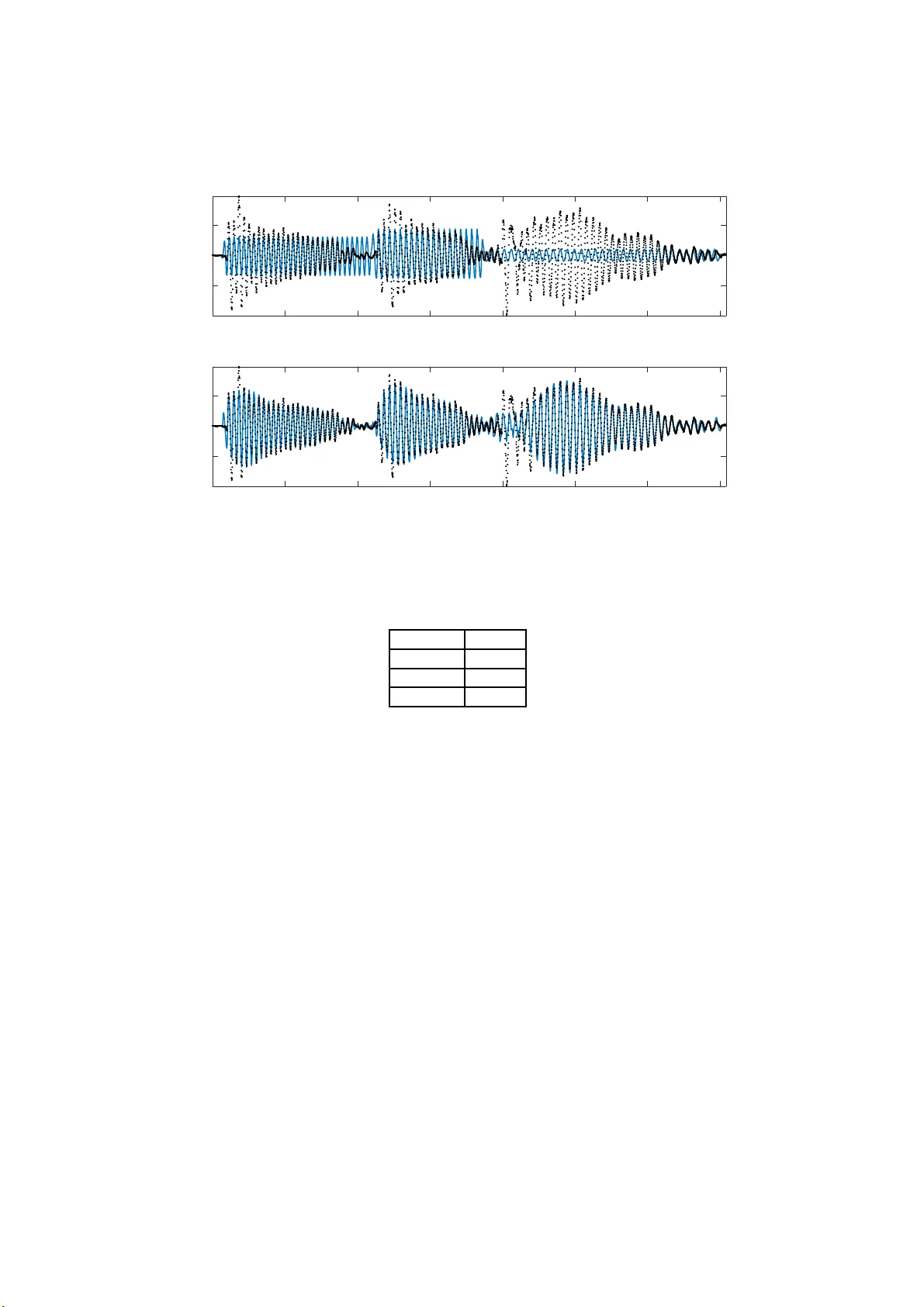
Loading high-quality paper...
Comments & Academic Discussion
Loading comments...
Leave a Comment