Learning to Optimize

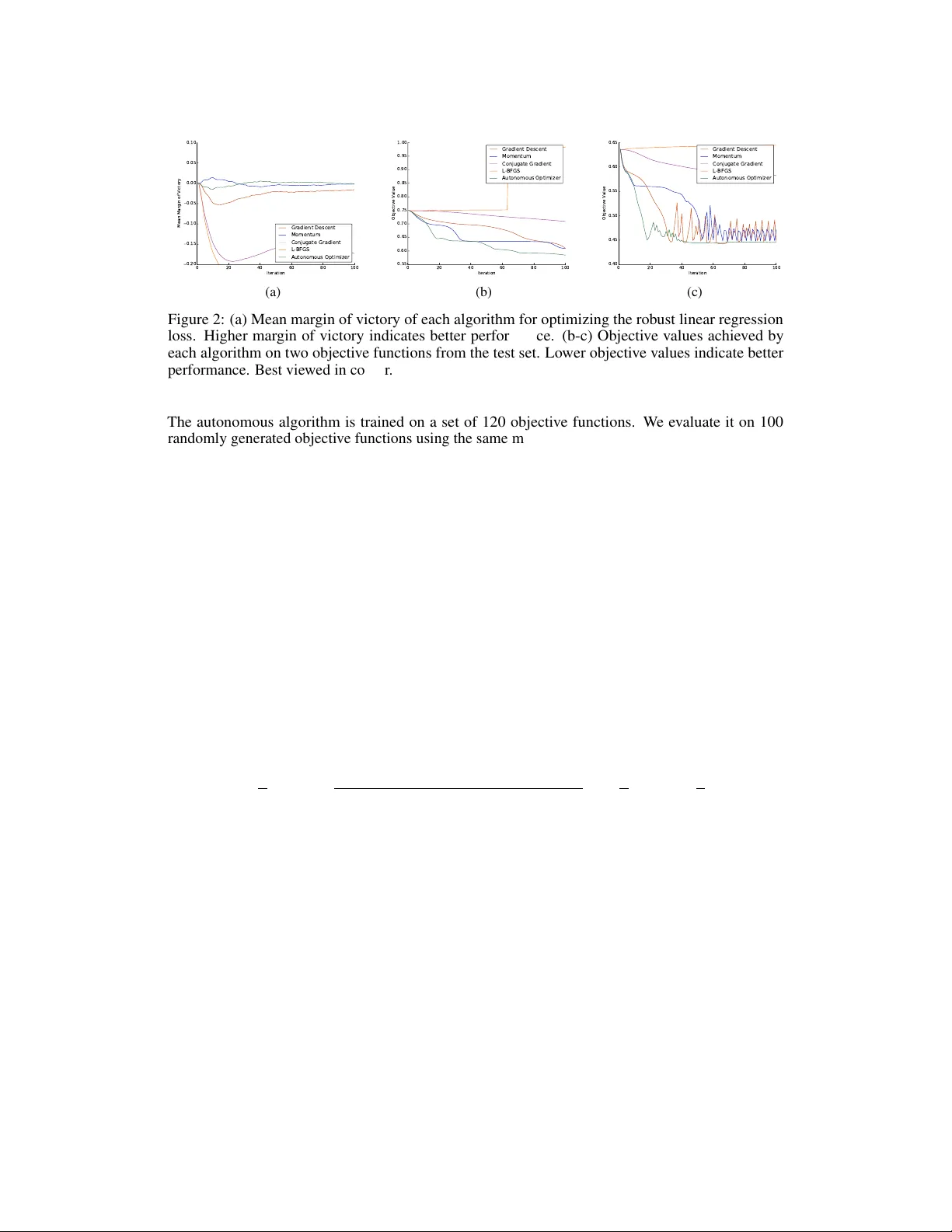
Lear ning to Optimize Ke Li Jitendra Malik Department of Electrical Engineering and Computer Sciences Univ ersity of California, Berkele y Berkeley , CA 94720 United States {ke.li,malik}@eecs.berkeley.edu Abstract Algorithm design is a laborious process and often requires many iterations of ideation and validation. In this paper , we explore automating algorithm design and present a method to learn an optimization algorithm, which we believ e to be the first method that can automatically discov er a better algorithm. W e approach this problem from a reinforcement learning perspectiv e and represent any particular optimization algorithm as a policy . W e learn an optimization algorithm using guided policy search and demonstrate that the resulting algorithm outperforms existing hand-engineered algorithms in terms of con vergence speed and/or the final objectiv e value. 1 Introduction The current approach to designing algorithms is a laborious process. First, the designer must study the problem and de vise an algorithm guided by a mixture of intuition, theoretical and/or empirical insight and general design paradigms. She then needs to analyze the algorithm’ s performance on prototypical examples and compare it to that of e xisting algorithms. If the algorithm falls short, she must uncov er the underlying cause and find cle ver w ays to overcome the disco vered shortcomings. She iterates on this process until she arriv es at an algorithm that is superior than existing algorithms. Giv en the often protracted nature of this process, a natural question to ask is: can we automate it? In this paper , we focus on automating the design of unconstrained continuous optimization algorithms, which are some of the most po werful and ubiquitous tools used in all areas of science and engineering. Extensi ve w ork o ver the past se veral decades has yielded many popular methods, like gradient descent, momentum, conjugate gradient and L-BFGS. These algorithms share one commonality: they are all hand-engineered – that is, the steps of these algorithms are carefully designed by human experts. Just as deep learning has achie ved tremendous success by automating feature engineering, automating algorithm design could open the way to similar performance gains. W e learn a better optimization algorithm by observing its e xecution. T o this end, we formulate the problem as a reinforcement learning problem. Under this frame work, an y particular optimization algorithm simply corresponds to a policy . W e re ward optimization algorithms that con ver ge quickly and penalize those that do not. Learning an optimization algorithm then reduces to finding an optimal policy , which can be solved using any reinforcement learning method. T o differentiate the algorithm that performs learning from the algorithm that is learned, we will henceforth refer to the former as the “learning algorithm” or “learner” and the latter as the “autonomous algorithm” or “policy”. W e use an off-the-shelf reinforcement learning algorithm kno wn as guided polic y search [ 17 ], which has demonstrated success in a v ariety of robotic control settings [ 18 , 10 , 19 , 12 ]. W e show empirically that the autonomous optimization algorithm we learn con verges f aster and/or finds better optima than existing hand-engineered optimization algorithms. 2 Related W ork Early work has e xplored the general theme of speeding up learning with accumulation of learning experience. This line of work, known as “learning to learn” or “meta-learning” [ 1 , 27 , 5 , 26 ], considers the problem of de vising methods that can take adv antage of knowledge learned on other related tasks to train faster , a problem that is today better kno wn as multi-task learning and transfer learning. In contrast, the proposed method can learn to accelerate the training procedure itself, without necessarily requiring any training on related auxiliary tasks. A different line of w ork, known as “programming by demonstration” [ 7 ], considers the problem of learning programs from e xamples of input and output. Several dif ferent approaches ha ve been proposed: Liang et al. [ 20 ] represents programs explicitly using a formal language, constructs a hierarchical Bayesian prior ov er programs and performs inference using an MCMC sampling procedure and Gra ves et al. [ 11 ] represents programs implicitly as sequences of memory access operations and trains a recurrent neural net to learn the underlying patterns in the memory access operations. Subsequent work proposes v ariants of this model that use different primiti ve memory access operations [ 14 ], more e xpressive operations [ 16 , 28 ] or other non-dif ferentiable operations [ 30 , 29 ]. Others consider b uilding models that permit parallel e xecution [ 15 ] or training models with stronger supervision in the form of ex ecution traces [ 23 ]. The aim of this line of work is to replicate the behaviour of simple existing algorithms from e xamples, rather than to learn a new algorithm that is better than existing algorithms. There is a rich body of work on hyperparameter optimization, which studies the optimization of hyperparameters used to train a model, such as the learning rate, the momentum decay factor and re gularization parameters. Most methods [ 13 , 4 , 24 , 25 , 9 ] rely on sequential model-based Bayesian optimization [ 22 , 6 ], while others adopt a random search approach [ 3 ] or use gradient- based optimization [ 2 , 8 , 21 ]. Because each hyperparameter setting corresponds to a particular instantiation of an optimization algorithm, these methods can be vie wed as a way to search o ver different instantiations of the same optimization algorithm. The proposed method, on the other hand, can search over the space of all possible optimization algorithms. In addition, when presented with a new objectiv e function, hyperparameter optimization needs to conduct multiple trials with different hyperparameter settings to find the optimal hyperparameters. In contrast, once training is complete, the autonomous algorithm kno ws ho w to choose hyperparameters on-the-fly without needing to try different h yperparameter settings, ev en when presented with an objecti ve function that it has not seen during training. T o the best of our kno wledge, the proposed method represents the first attempt to learn a better algorithm automatically . 3 Method 3.1 Preliminaries In the reinforcement learning setting, the learner is gi ven a choice of actions to tak e in each time step, which changes the state of the en vironment in an unknown fashion, and recei ves feedback based on the consequence of the action. The feedback is typically gi ven in the form of a re ward or cost, and the objecti ve of the learner is to choose a sequence of actions based on observ ations of the current en vironment that maximizes cumulative re ward or minimizes cumulati ve cost over all time steps. A reinforcement learning problem is typically formally represented as an Mark ov decision process (MDP). W e consider a finite-horizon MDP with continuous state and action spaces defined by the tuple ( S , A , p 0 , p, c, γ ) , where S is the set of states, A is the set of actions, p 0 : S → R + is the probability density ov er initial states, p : S × A × S → R + is the transition probability density , that is, the conditional probability density o ver successor states gi ven the current state and action, c : S → R is a function that maps state to cost and γ ∈ (0 , 1] is the discount f actor . The objectiv e is to learn a stochastic policy π ∗ : S × A → R + , which is a conditional probability density o ver actions giv en the current state, such that the expected cumulative cost is minimized. That 2 is, π ∗ = arg min π E s 0 ,a 0 ,s 1 ,...,s T " T X t =0 γ t c ( s t ) # , where the expectation is taken with respect to the joint distrib ution ov er the sequence of states and actions, often referred to as a trajectory , which has the density q ( s 0 , a 0 , s 1 , . . . , s T ) = p 0 ( s 0 ) T − 1 Y t =0 π ( a t | s t ) p ( s t +1 | s t , a t ) . This problem of finding the cost-minimizing policy is known as the policy search problem. T o enable generalization to unseen states, the policy is typically parameterized and minimization is performed ov er representable policies. Solving this problem exactly is intractable in all but selected special cases. Therefore, policy search methods generally tackle this problem by solving it approximately . In many practical settings, p , which characterizes the dynamics, is unkno wn and must therefore be estimated. Additionally , because it is often equally important to minimize cost at earlier and later time steps, we will henceforth focus on the undiscounted setting, i.e. the setting where γ = 1 . Guided policy search [ 17 ] is a method for performing policy search in continuous state and action spaces under possibly unkno wn dynamics. It works by alternating between computing a target distribution o ver trajectories that is encouraged to minimize cost and agree with the current polic y and learning parameters of the policy in a standard supervised fashion so that sample trajectories from executing the policy are close to sample trajectories drawn from the target distribution. The target trajectory distrib ution is computed by iterativ ely fitting local time-varying linear and quadratic approximations to the (estimated) dynamics and cost respectiv ely and optimizing over a restricted class of linear-Gaussian policies subject to a trust region constraint, which can be solved ef ficiently in closed form using a dynamic programming algorithm known as linear -quadratic-Gaussian (LQG). W e refer interested readers to [17] for details. 3.2 Formulation Consider the general structure of an algorithm for unconstrained continuous optimization, which is outlined in Algorithm 1. Starting from a random location in the domain of the objective function, the algorithm iterativ ely updates the current location by a step vector computed from some functional π of the objectiv e function, the current location and past locations. Algorithm 1 General structure of optimization algorithms Require: Objectiv e function f x (0) ← random point in the domain of f for i = 1 , 2 , . . . do ∆ x ← π ( f , { x (0) , . . . , x ( i − 1) } ) if stopping condition is met then retur n x ( i − 1) end if x ( i ) ← x ( i − 1) + ∆ x end for This frame work subsumes all existing optimization algorithms. Different optimization algorithms dif fer in the choice of π . First-order methods use a π that depends only on the gradient of the objecti ve function, whereas second-order methods use a π that depends on both the gradient and the Hessian of the objectiv e function. In particular , the follo wing choice of π yields the gradient descent method: π ( f , { x (0) , . . . , x ( i − 1) } ) = − γ ∇ f ( x ( i − 1) ) , where γ denotes the step size or learning rate. Similarly , the following choice of π yields the gradient descent method with momentum: π ( f , { x (0) , . . . , x ( i − 1) } ) = − γ   i − 1 X j =0 α i − 1 − j ∇ f ( x ( j ) )   , 3 where γ again denotes the step size and α denotes the momentum decay factor . Therefore, if we can learn π , we will be able to learn an optimization algorithm. Since it is dif ficult to model general functionals, in practice, we restrict the dependence of π on the objecti ve function f to objecti ve v alues and gradients ev aluated at current and past locations. Hence, π can be simply modelled as a function from the objective values and gradients along the trajectory taken by the optimizer so far to the next step v ector . W e observe that the execution of an optimization algorithm can be viewed as the execution of a fixed policy in an MDP: the state consists of the current location and the objectiv e v alues and gradients e valuated at the current and past locations, the action is the step vector that is used to update the current location, and the transition probability is partially characterized by the location update formula, x ( i ) ← x ( i − 1) + ∆ x . The policy that is e xecuted corresponds precisely to the choice of π used by the optimization algorithm. For this reason, we will also use π to denote the policy at hand. Under this formulation, searching over policies corresponds to searching o ver all possible first-order optimization algorithms. W e can use reinforcement learning to learn the policy π . T o do so, we need to define the cost function, which should penalize policies that exhibit undesirable behaviours during their ex ecution. Since the performance metric of interest for optimization algorithms is the speed of con vergence, the cost function should penalize policies that conv erge slowly . T o this end, assuming the goal is to minimize the objectiv e function, we define cost at a state to be the objectiv e value at the current location. This encourages the policy to reach the minimum of the objecti ve function as quickly as possible. Since the policy π may be stochastic in general, we model each dimension of the action conditional on the state as an independent Gaussian whose mean is given by a regression model and variance is some learned constant. W e choose to parameterize the mean of π using a neural net, due to its appealing properties as a uni versal function approximator and strong empirical performance in a variety of applications. W e use guided policy search to learn the parameters of the polic y . W e use a training set consisting of different randomly generated objectiv e functions. W e e v aluate the resulting autonomous algorithm on different objecti ve functions drawn from the same distrib ution. 3.3 Discussion An autonomous optimization algorithm of fers sev eral advantages ov er hand-engineered algorithms. First, an autonomous optimizer is trained on real algorithm execution data, whereas hand-engineered optimizers are typically derived by analyzing objecti ve functions with properties that may or may not be satisfied by objectiv e functions that arise in practice. Hence, an autonomous optimizer minimizes the amount of a priori assumptions made about objecti ve functions and can instead take full adv antage of the information about the actual objective functions of interest. Second, an autonomous optimizer has no hyperparameters that need to be tuned by the user . Instead of just computing a step direction which must then be combined with a user -specified step size, an autonomous optimizer predicts the step direction and size jointly . This allows the autonomous optimizer to dynamically adjust the step size based on the information it has acquired about the objectiv e function while performing the optimization. Finally , when an autonomous optimizer is trained on a particular class of objecti ve functions, it may be able to discov er hidden structure in the geometry of the class of objectiv e functions. At test time, it can then exploit this kno wledge to perform optimization faster . 3.4 Implementation Details W e store the current location, pre vious gradients and improvements in the objecti ve v alue from previous iterations in the state. W e keep track of only the information pertaining to the pre vious H time steps and use H = 25 in our experiments. More specifically , the dimensions of the state space encode the following information: • Current location in the domain • Change in the objective v alue at the current location relative to the objecti ve value at the i th most recent location for all i ∈ { 2 , . . . , H + 1 } • Gradient of the objecti ve function e valuated at the i th most recent location for all i ∈ { 2 , . . . , H + 1 } 4 Initially , we set the dimensions corresponding to historical information to zero. The current location is only used to compute the cost; because the policy should not depend on the absolute coordinates of the current location, we exclude it from the input that is fed into the neural net. W e use a small neural net to model the policy . Its architecture consists of a single hidden layer with 50 hidden units. Softplus activ ation units are used in the hidden layer and linear activ ation units are used in the output layer . The training objectiv e imposed by guided polic y search takes the form of the squared Mahalanobis distance between mean predicted and target actions along with other terms dependent on the v ariance of the policy . W e also regularize the entropy of the policy to encourage deterministic actions conditioned on the state. The coefficient on the re gularizer increases gradually in later iterations of guided polic y search. W e initialize the weights of the neural net randomly and do not regularize the magnitude of weights. Initially , we set the tar get trajectory distrib ution so that the mean action given state at each time step matches the step vector used by the gradient descent method with momentum. W e choose the best settings of the step size and momentum decay factor for each objecti ve function in the training set by performing a grid search o ver hyperparameters and running noiseless gradient descent with momentum for each hyperparameter setting. For training, we sample 20 trajectories with a length of 40 time steps for each objecti ve function in the training set. After each iteration of guided policy search, we sample new trajectories from the new distrib ution and discard the trajectories from the preceding iteration. 4 Experiments W e learn autonomous optimization algorithms for v arious con vex and non-con ve x classes of objecti ve functions that correspond to loss functions for dif ferent machine learning models. W e first learn an autonomous optimizer for logistic re gression, which induces a con vex loss function. W e then learn an autonomous optimizer for rob ust linear regression using the Geman-McClure M-estimator , whose loss function is non-con vex. Finally , we learn an autonomous optimizer for a tw o-layer neural net classifier with ReLU activ ation units, whose error surface has e ven more complex geometry . 4.1 Logistic Regression W e consider a logistic regression model with an ` 2 regularizer on the weight vector . Training the model requires optimizing the following objecti ve: min w ,b − 1 n n X i =1 y i log σ  w T x i + b  + (1 − y i ) log  1 − σ  w T x i + b  + λ 2 k w k 2 2 , where w ∈ R d and b ∈ R denote the weight vector and bias respecti vely , x i ∈ R d and y i ∈ { 0 , 1 } denote the feature vector and label of the i th instance, λ denotes the coef ficient on the regularizer and σ ( z ) : = 1 1+ e − z . For our experiments, we choose λ = 0 . 0005 and d = 3 . This objectiv e is con vex in w and b . W e train an autonomous algorithm that learns to optimize objectiv es of this form. The training set consists of examples of such objecti ve functions whose free v ariables, which in this case are x i and y i , are all assigned concrete values. Hence, each objectiv e function in the training set corresponds to a logistic regression problem on a dif ferent dataset. T o construct the training set, we randomly generate a dataset of 100 instances for each function in the training set. The instances are drawn randomly from two multi variate Gaussians with random means and cov ariances, with half drawn from each. Instances from the same Gaussian are assigned the same label and instances from different Gaussians are assigned dif ferent labels. W e train the autonomous algorithm on a set of 90 objectiv e functions. W e ev aluate it on a test set of 100 random objecti ve functions generated using the same procedure and compare to popular hand-engineered algorithms, such as gradient descent, momentum, conjugate gradient and L-BFGS. All baselines are run with the best hyperparameter settings tuned on the training set. For each algorithm and objective function in the test set, we compute the difference between the objectiv e value achiev ed by a given algorithm and that achiev ed by the best of the competing 5 0 20 40 60 80 100 Iteration 0.20 0.15 0.10 0.05 0.00 0.05 0.10 Mean Margin of Victory Gradient Descent Momentum Conjugate Gradient L-BFGS Autonomous Optimizer (a) 0 20 40 60 80 100 Iteration 0.52 0.53 0.54 0.55 0.56 0.57 0.58 Objective Value Gradient Descent Momentum Conjugate Gradient L-BFGS Autonomous Optimizer (b) 0 20 40 60 80 100 Iteration 0.1 0.2 0.3 0.4 0.5 0.6 0.7 0.8 Objective Value Gradient Descent Momentum Conjugate Gradient L-BFGS Autonomous Optimizer (c) Figure 1: (a) Mean margin of victory of each algorithm for optimizing the logistic regression loss. Higher margin of victory indicates better performance. (b-c) Objective values achie ved by each algorithm on two objecti ve functions from the test set. Lower objecti ve values indicate better performance. Best viewed in colour . algorithms at every iteration, a quantity we will refer to as “the margin of victory”. This quantity is positi ve when the current algorithm is better than all other algorithms and neg ativ e otherwise. In Figure 1a, we plot the mean mar gin of victory of each algorithm at each iteration a veraged over all objecti ve functions in the test set. W e find that conjugate gradient and L-BFGS diver ge or oscillate in rare cases (on 6% of the objecti ve functions in the test set), ev en though the autonomous algorithm, gradient descent and momentum do not. T o reflect performance of these baselines in the majority of cases, we exclude the of fending objective functions when computing the mean mar gin of victory . As shown, the autonomous algorithm outperforms gradient descent, momentum and conjugate gradient at almost e very iteration. The mar gin of victory of the autonomous algorithm is quite high in early iterations, indicating that the autonomous algorithm con ver ges much faster than other algorithms. It is interesting to note that despite having seen only trajectories of length 40 at training time, the autonomous algorithm is able to generalize to much longer time horizons at test time. L-BFGS conv erges to slightly better optima than the autonomous algorithm and the momentum method. This is not surprising, as the objecti ve functions are con ve x and L-BFGS is known to be a very good optimizer for con ve x optimization problems. W e show the performance of each algorithm on two objecti ve functions from the test set in Figures 1b and 1c. In Figure 1b, the autonomous algorithm con verges faster than all other algorithms. In Figure 1c, the autonomous algorithm initially con ver ges faster than all other algorithms but is later ov ertaken by L-BFGS, while remaining faster than all other optimizers. Howe ver , it ev entually achie ves the same objectiv e v alue as L-BFGS, while the objective values achieved by gradient descent and momentum remain much higher . 4.2 Robust Linear Regr ession Next, we consider the problem of linear re gression using a robust loss function. One way to ensure robustness is to use an M-estimator for parameter estimation. A popular choice is the Geman-McClure estimator , which induces the following objecti ve: min w ,b 1 n n X i =1  y i − w T x i − b  2 c 2 + ( y i − w T x i − b ) 2 , where w ∈ R d and b ∈ R denote the weight vector and bias respecti vely , x i ∈ R d and y i ∈ R denote the feature vector and label of t he i th instance and c ∈ R is a constant that modulates the shape of the loss function. For our experiments, we use c = 1 and d = 3 . This loss function is not con vex in either w or b . As with the preceding section, each objecti ve function in the training set is a function of the abo ve form with realized values for x i and y i . The dataset for each objective function is generated by drawing 25 random samples from each one of four multi variate Gaussians, each of which has a random mean and the identity cov ariance matrix. F or all points drawn from the same Gaussian, their labels are generated by projecting them along the same random vector , adding the same randomly generated bias and perturbing them with i.i.d. Gaussian noise. 6 0 20 40 60 80 100 Iteration 0.20 0.15 0.10 0.05 0.00 0.05 0.10 Mean Margin of Victory Gradient Descent Momentum Conjugate Gradient L-BFGS Autonomous Optimizer (a) 0 20 40 60 80 100 Iteration 0.55 0.60 0.65 0.70 0.75 0.80 0.85 0.90 0.95 1.00 Objective Value Gradient Descent Momentum Conjugate Gradient L-BFGS Autonomous Optimizer (b) 0 20 40 60 80 100 Iteration 0.40 0.45 0.50 0.55 0.60 0.65 Objective Value Gradient Descent Momentum Conjugate Gradient L-BFGS Autonomous Optimizer (c) Figure 2: (a) Mean margin of victory of each algorithm for optimizing the rob ust linear regression loss. Higher margin of victory indicates better performance. (b-c) Objective values achie ved by each algorithm on two objecti ve functions from the test set. Lower objecti ve values indicate better performance. Best viewed in colour . The autonomous algorithm is trained on a set of 120 objectiv e functions. W e ev aluate it on 100 randomly generated objectiv e functions using the same metric as above. As shown in Figure 2a, the autonomous algorithm outperforms all hand-engineered algorithms except at early iterations. While it dominates gradient descent, conjugate gradient and L-BFGS at all times, it does not make progress as quickly as the momentum method initially . Howe ver , after around 30 iterations, it is able to close the gap and surpass the momentum method. On this optimization problem, both conjugate gradient and L-BFGS div erge quickly . Interestingly , unlike in the previous e xperiment, L-BFGS no longer performs well, which could be caused by non-con vexity of the objecti ve functions. Figures 2b and 2c show performance on objectiv e functions from the test set. In Figure 2b, the autonomous optimizer not only conv erges the fastest, but also reaches a better optimum than all other algorithms. In Figure 2c, the autonomous algorithm conv erges the fastest and is able to avoid most of the oscillations that hamper gradient descent and momentum after reaching the optimum. 4.3 Neural Net Classifier Finally , we train an autonomous algorithm to train a small neural net classifier . W e consider a two-layer neural net with ReLU acti vation on the hidden units and softmax acti vation on the output units. W e use the cross-entropy loss combined with ` 2 regularization on the weights. T o train the model, we need to optimize the following objecti ve: min W,U , b , c − 1 n n X i =1 log   exp  ( U max ( W x i + b , 0) + c ) y i  P j exp  ( U max ( W x i + b , 0) + c ) j    + λ 2 k W k 2 F + λ 2 k U k 2 F , where W ∈ R h × d , b ∈ R h , U ∈ R p × h , c ∈ R p denote the first-layer and second-layer weights and biases, x i ∈ R d and y i ∈ { 1 , . . . , p } denote the input and target class label of the i th instance, λ denotes the coef ficient on re gularizers and ( v ) j denotes the j th component of v . For our experiments, we use λ = 0 . 0005 and d = h = p = 2 . The error surface is kno wn to have comple x geometry and multiple local optima, making this a challenging optimization problem. The training set consists of 80 objective functions, each of which corresponds to the objective for training a neural net on a different dataset. Each dataset is generated by generating four multiv ariate Gaussians with random means and cov ariances and sampling 25 points from each. The points from the same Gaussian are assigned the same random label of either 0 or 1. W e make sure not all of the points in the dataset are assigned the same label. W e ev aluate the autonomous algorithm in the same manner as above. As shown in Figure 3a, the autonomous algorithm significantly outperforms all other algorithms. In particular , as evidenced by the sizeable and sustained gap between mar gin of victory of the autonomous optimizer and the momentum method, the autonomous optimizer is able to reach much better optima and is less prone to getting trapped in local optima compared to other methods. This gap is also larger compared to that exhibited in pre vious sections, suggesting that hand-engineered algorithms are more sub-optimal on 7 0 20 40 60 80 100 Iteration 0.20 0.15 0.10 0.05 0.00 0.05 0.10 Mean Margin of Victory Gradient Descent Momentum Conjugate Gradient L-BFGS Autonomous Optimizer (a) 0 20 40 60 80 100 Iteration 0.4 0.6 0.8 1.0 1.2 1.4 Objective Value Gradient Descent Momentum Conjugate Gradient L-BFGS Autonomous Optimizer (b) 0 20 40 60 80 100 Iteration 0.4 0.6 0.8 1.0 1.2 1.4 1.6 Objective Value Gradient Descent Momentum Conjugate Gradient L-BFGS Autonomous Optimizer (c) Figure 3: (a) Mean margin of victory of each algorithm for training neural net classifiers. Higher margin of victory indicates better performance. (b-c) Objecti ve values achie ved by each algorithm on two objecti ve functions from the test set. Lower objecti ve v alues indicate better performance. Best viewed in colour . challenging optimization problems and so the potential for improvement from learning the algorithm is greater in such settings. Due to non-con ve xity , conjugate gradient and L-BFGS often div erge. Performance on examples of objecti ve functions from the test set is shown in Figures 3b and 3c. As shown, the autonomous optimizer is able to reach better optima than all other methods and lar gely av oids oscillations that other methods suffer from. 5 Conclusion W e presented a method for learning a better optimization algorithm. W e formulated this as a reinforcement learning problem, in which any optimization algorithm can be represented as a policy . Learning an optimization algorithm then reduces to find the optimal policy . W e used guided polic y search for this purpose and trained autonomous optimizers for different classes of con ve x and non- con vex objecti ve functions. W e demonstrated that the autonomous optimizer con verges f aster and/or reaches better optima than hand-engineered optimizers. W e hope autonomous optimizers learned using the proposed approach can be used to solve various common classes of optimization problems more quickly and help accelerate the pace of innov ation in science and engineering. References [1] Jonathan Baxter, Rich Caruana, T om Mitchell, Lorien Y Pratt, Daniel L Silver , and Sebastian Thrun. NIPS 1995 workshop on learning to learn: Kno wledge consolidation and transfer in inductiv e sys- tems. https://web.archive.org/web/20000618135816/http://www.cs.cmu.edu/afs/cs.cmu. edu/user/caruana/pub/transfer.html , 1995. Accessed: 2015-12-05. [2] Y oshua Bengio. Gradient-based optimization of hyperparameters. Neural computation , 12(8):1889–1900, 2000. [3] James Bergstra and Y oshua Bengio. Random search for hyper-parameter optimization. The J ournal of Machine Learning Resear ch , 13(1):281–305, 2012. [4] James S Bergstra, Rémi Bardenet, Y oshua Bengio, and Balázs Kégl. Algorithms for hyper-parameter optimization. In Advances in Neur al Information Processing Systems , pages 2546–2554, 2011. [5] Pa vel Brazdil, Christophe Giraud Carrier, Carlos Soares, and Ricardo V ilalta. Metalearning: applications to data mining . Springer Science & Business Media, 2008. [6] Eric Brochu, Vlad M Cora, and Nando De Freitas. A tutorial on bayesian optimization of expensi ve cost functions, with application to active user modeling and hierarchical reinforcement learning. arXiv preprint arXiv:1012.2599 , 2010. [7] Allen Cypher and Daniel Conrad Halbert. W atch what I do: pr ogramming by demonstr ation . MIT press, 1993. [8] Justin Domke. Generic methods for optimization-based modeling. In AIST ATS , v olume 22, pages 318–326, 2012. [9] Matthias Feurer , Jost T obias Springenberg, and Frank Hutter . Initializing bayesian hyperparameter optimization via meta-learning. In AAAI , pages 1128–1135, 2015. 8 [10] Chelsea Finn, Xin Y u T an, Y an Duan, T revor Darrell, Serge y Le vine, and Pieter Abbeel. Learning visual feature spaces for robotic manipulation with deep spatial autoencoders. arXiv pr eprint arXiv:1509.06113 , 2015. [11] Alex Gra ves, Greg W ayne, and Ivo Danihelka. Neural Turing machines. arXiv pr eprint arXiv:1410.5401 , 2014. [12] W eiqiao Han, Ser gey Le vine, and Pieter Abbeel. Learning compound multi-step controllers under unkno wn dynamics. In International Confer ence on Intelligent Robots and Systems , 2015. [13] Frank Hutter , Holger H Hoos, and K evin Le yton-Brown. Sequential model-based optimization for general algorithm configuration. In Learning and Intellig ent Optimization , pages 507–523. Springer, 2011. [14] Armand Joulin and T omas Mikolov . Inferring algorithmic patterns with stack-augmented recurrent nets. In Advances in Neural Information Pr ocessing Systems , pages 190–198, 2015. [15] Łukasz Kaiser and Ilya Sutske ver . Neural gpus learn algorithms. arXiv preprint , 2015. [16] Karol Kurach, Marcin Andrycho wicz, and Ilya Sutskev er . Neural random-access machines. arXiv preprint arXiv:1511.06392 , 2015. [17] Serge y Levine and Pieter Abbeel. Learning neural network policies with guided policy search under unknown dynamics. In Advances in Neural Information Pr ocessing Systems , pages 1071–1079, 2014. [18] Serge y Le vine, Chelsea Finn, T revor Darrell, and Pieter Abbeel. End-to-end training of deep visuomotor policies. arXiv pr eprint arXiv:1504.00702 , 2015. [19] Serge y Le vine, Nolan W agener, and Pieter Abbeel. Learning contact-rich manipulation skills with guided policy search. arXiv preprint , 2015. [20] Percy Liang, Michael I Jordan, and Dan Klein. Learning programs: A hierarchical Bayesian approach. In Pr oceedings of the 27th International Confer ence on Machine Learning (ICML-10) , pages 639–646, 2010. [21] Dougal Maclaurin, Da vid Duvenaud, and Ryan P Adams. Gradient-based h yperparameter optimization through rev ersible learning. arXiv pr eprint arXiv:1502.03492 , 2015. [22] Jonas Mockus, Vytautas T iesis, and Antanas Zilinskas. The application of bayesian methods for seeking the extremum. T owards global optimization , 2(117-129):2, 1978. [23] Scott Reed and Nando de Freitas. Neural programmer-interpreters. arXiv pr eprint arXiv:1511.06279 , 2015. [24] Jasper Snoek, Hugo Larochelle, and Ryan P Adams. Practical bayesian optimization of machine learning algorithms. In Advances in neur al information processing systems , pages 2951–2959, 2012. [25] Ke vin Swersky , Jasper Snoek, and Ryan P Adams. Multi-task bayesian optimization. In Advances in neural information pr ocessing systems , pages 2004–2012, 2013. [26] Sebastian Thrun and Lorien Pratt. Learning to learn . Springer Science & Business Media, 2012. [27] Ricardo V ilalta and Y oussef Drissi. A perspecti ve vie w and surve y of meta-learning. Artificial Intellig ence Revie w , 18(2):77–95, 2002. [28] Greg Y ang. Lie access neural turing machine. arXiv preprint arXiv:1602.08671 , 2016. [29] W ojciech Zaremba, T omas Mikolo v , Armand Joulin, and Rob Fer gus. Learning simple algorithms from examples. arXiv preprint , 2015. [30] W ojciech Zaremba and Ilya Sutskev er . Reinforcement learning neural turing machines. arXiv preprint arXiv:1505.00521 , 2015. 9