Semidefinite Programs for Exact Recovery of a Hidden Community

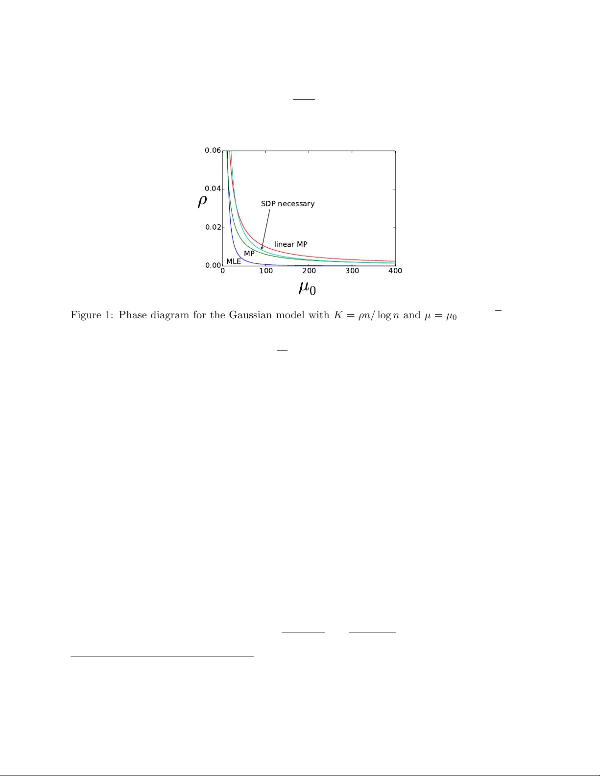
Semideﬁnite Programs for Exact Reco v ery of a Hidden Comm unit y Bruce Ha jek Yihong W u Jiaming Xu ∗ No vem b er 14, 2021 Abstract W e study a semideﬁnite programming (SDP) relaxation of the maxim um likelihoo d estimation for exactly recov ering a hidden communit y of cardinality K from an n × n symmetric data matrix A , where for distinct indices i, j , A ij ∼ P if i, j are b oth in the comm unity and A ij ∼ Q otherwise, for t wo kno wn probability distributions P and Q . W e iden tify a suﬃcient condition and a necessary condition for the success of SDP for the general mo del. F or b oth the Bernoulli case ( P = Bern ( p ) and Q = Bern ( q ) with p > q ) and the Gaussian case ( P = N ( µ, 1) and Q = N (0 , 1) with µ > 0), whic h corresp ond to the problem of plan ted dense subgraph recov ery and submatrix localization resp ectively , the general results lead to the follo wing ﬁndings: (1) If K = ω ( n/ log n ), SDP attains the information-theoretic recov ery limits with sharp constants; (2) If K = Θ( n/ log n ), SDP is order-wise optimal, but strictly sub optimal by a constant factor; (3) If K = o ( n/ log n ) and K → ∞ , SDP is order-wise sub optimal. The same critical scaling for K is found to hold, up to constant factors, for the p erformance of SDP on the sto chastic blo ck mo del of n v ertices partitioned into multiple communities of equal size K . A key ingredient in the pro of of the necessary condition is a construction of a primal feasible solution based on random p erturbation of the true cluster matrix. 1 In tro duction 1.1 Motiv ation and problem setup Consider the sto chastic blo ck mo del (SBM) [ 24 ] with a single comm unity , where out of n v ertices a comm unity consisting of K v ertices are chosen uniformly at random; tw o vertices are connected b y an edge with probabilit y p if they both b elong to the comm unity and with probabilit y q if either one of them is not in the communit y . The goal is to recov er the communit y based on observ ation of the graph, which, when p > q , is also known as the plante d dense sub gr aph recov ery problem [ 32 , 10 , 19 , 34 ]. In the sp ecial case of p = 1 and q = 1 / 2, planted dense subgraph reco very reduces to the widely-studied planted clique problem, i.e., ﬁnding a hidden clique of size K in the Erd˝ os-R ´ en yi random graph G ( n, 1 / 2). It is well-kno wn that the maximum likelihoo d estimator (MLE), which is computationally intractable, ﬁnds any clique of size K ≥ 2(1 +  ) log 2 n for any constant  > 0; ho wev er, existing p olynomial-time algorithms, including sp ectral metho ds [ 2 ], message passing [ 14 ], and s emi-deﬁnite programming (SDP) relaxation of MLE [ 16 ], are only known to ﬁnd a clique of size K ≥  √ n . In fact, imp ossibilit y results for the more p ow erful s -round Lo v´ asz-Sc hrijv er relaxations and, more recen tly , degree-2 r sums-of-squares (SOS) relaxation (with s = 1 and r = 1 corresp onding ∗ B. Ha jek and Y. W u are with the Department of ECE and Co ordinated Science Lab, Universit y of Illinois at Urbana-Champaign, Urbana, IL, { b-hajek,yihongwu } @illinois.edu . J. Xu is with the Simons Institute for the Theory of Computing, Univ ersity of California, Berk eley , Berkeley , CA, jiamingxu@berkeley.edu . 1 to SDP) hav e b een recen tly obtained in [ 17 ] and [ 15 , 33 , 25 , 37 ], showing that relaxations of constant rounds or degrees lead to order-wise sub optimality even for detecting the clique. In other words, for the planted clique problem there is a signiﬁcant gap b etw een the state of the art of p olynomial-time algorithms and what is information-theoretically p ossible. In sharp contrast, for sparser graphs and larger comm unity size, SDP relaxations ha ve b een sho wn to achiev e the information-theoretic recov ery limit up to sharp constants. F or p = a log n/n, q = b log n/n and K = ρn for ﬁxed constants a, b > 0 and 0 < ρ < 1, the recent work [ 23 ] identiﬁed a sharp threshold ρ ∗ = ρ ∗ ( a, b ) such that if ρ > ρ ∗ , an SDP relaxation of MLE recov ers the hidden comm unity with high probability; if ρ < ρ ∗ , exact recov ery is information theoretically imp ossible. This optimality result of SDP has b een extended to multiple communities as long as their sizes scale linearly with the graph size n [ 4 , 18 , 1 , 36 , 35 ]. The dic hotomy b etw een the optimalit y of SDP up to sharp constants in the relatively sparse regime and the order-wise sub optimalit y of SDP in the dense regime prompts us to inv estigate the follo wing question: When do SDP r elaxations c e ase to b e optimal for plante d dense sub gr aph r e c overy ? In this pap er, w e address this question under the more general hidden comm unity mo del considered in [ 14 ]. Deﬁnition 1 (Hidden Comm unity Mo del) . Let C ∗ b e dra wn uniformly at random from all subsets of [ n ] of cardinality K . Giv en probabilit y measures P and Q on a common measurable space X , let A b e an n × n symmetric matrix with zero diagonal where for all 1 ≤ i < j ≤ n , A ij are m utually indep enden t, and A ij ∼ P if i, j ∈ C ∗ and A ij ∼ Q otherwise. The distributions P and Q as well as the comm unity size K v ary with the matrix size n in general. In this pap er we assume that these mo del parameters are known to the estimator, and fo cus on exact recov ery of the hidden communit y based on the data matrix A , namely , constructing an estimator b C = b C ( A ), suc h that as n → ∞ , P { b C 6 = C ∗ } → 0 uniformly in the choice of the true cluster C ∗ . W e are particularly interested in the following choices of P and Q : • Bernoulli case: P = Bern ( p ) and Q = Bern ( q ) with 0 ≤ q < p ≤ 1. In this case, the data matrix A corresp onds to the adjacency matrix of a graph, and the problem reduces to planted dense subgraph reco very . • Gaussian case: P = N ( µ, 1) and Q = N (0 , 1) with µ > 0. In this case, the submatrix of A with row and column indices in C ∗ has a p ositive mean µ except on the diagonal, while the rest of A has zero mean, and the problem corresp onds to a symmetric version of the submatrix lo c alization problem studied in [ 38 , 27 , 8 , 31 , 10 , 9 ]. 1.2 Main results W e show that for b oth plan ted dense subgraph recov ery and submatrix lo calization, SDP relaxations of MLE achiev e the information-theoretic optimal threshold if and only if the hidden communit y size satisﬁes K = ω ( n log n ). More sp eciﬁcally , • K = ω ( n log n ), SDP attains the information-theoretic recov ery limits with sharp constants. This extends the previous result in [ 23 ] obtained for K = Θ( n ) and the Bernoulli case. • K = Θ( n log n ), SDP is order-wise optimal, but strictly sub optimal by a constant factor; 2 • K = o ( n log n ) and K → ∞ , SDP is order-wise sub optimal. T o establish our main results, w e derive a suﬃcient condition and a necessary condition under whic h the optimal solution to SDP is unique and coincides with the true cluster matrix. In particular, for planted dense subgraph reco very , whenev er SDP do es not ac hieve the information-theoretic threshold, our suﬃcient condition and necessary condition are within constant factors of each other; for submatrix lo calization, we c haracterize the minimal signal-to-noise ratio required b y SDP within a factor of four when K = ω ( √ n ). The suﬃciency pro of is similar to those in [ 23 ] based on the dual certiﬁcate argumen t; we extend the construction and v alidation of dual certiﬁcates for the success of SDP to the general distributions P , Q . The necessity pro of is via constructing a high-probabilit y feasible solution to the SDP by means of random p erturbation of the ground truth that leads to a higher ob jectiv e v alue. One could instead adapt the existing constructions in the SOS literature for planted clique [ 15 , 33 , 25 , 37 ] to our setting, but it falls short of establishing the imp ossibility of SDP to attain the optimal recov ery threshold in the critical regime of K = Θ( n/ log n ); see Remark 2 for details. An alternative approach to establish imp ossibility results for SDP , thanks to strong duality that holds for the sp eciﬁc program, is to pro ve the non-existence of dual certiﬁcates, which turns out to yield the same condition given by the aforemen tioned explicit construction of primal solutions. The dual-based metho d has b een previously used for proving necessary conditions for related n uclear-norm constrained optimization problems, see e.g., [ 27 , 40 , 10 ]; how ev er, the constants in the deriv ed conditions are often lo ose or unsp eciﬁed. In comparison, we aim to obtain necessary conditions for SDP relaxations with explicit constan ts. Another diﬀerence is that the sp eciﬁc SDP considered here is more complicated inv olving the stringen t p ositiv e semi-deﬁnite constraint and a set of equalit y and non-negativity constraints. Using similar techniques, w e obtain analogous results for SDP relaxation for SBM with logarith- mically many communities. Sp eciﬁcally , consider the net work of n = r K v ertices partitioned in to r comm unities of cardinalit y K eac h, with edge probability p for pairs of v ertices within comm unities and q for other pairs of vertices. Then SDP relaxation, in contrast to the MLE, is constant wise sub optimal if r ≥ C log n for suﬃciently large C , and orderwise sub optimal if r = ω (log n ) . That is, it is constant wise sub optimal if K ≤ cn log n for suﬃciently small c , and orderwise sub optimal if K = o  n log n  . This result complements the sharp optimalit y for SDP previously established in [ 18 ] for r = O (1) and extended to r = o (log n ) in [ 1 ]. In closing, we comment on the barrier which preven ts SDP from b eing optimal. It is known that, see e.g., [ 10 , 35 ], sp ectral metho ds which estimate the comm unities based on the leading eigenv ector of the data matrix A suﬀer from a sp ectral barrier: the sp ectrum of the “signal part” E [ A ] m ust escap e that of the “noise part” A − E [ A ] , i.e., the smallest nonzero singular v alue of E [ A ] needs to b e muc h larger than the sp ectral norm k A − E [ A ] k . Closely related to the sp ectral barrier, the SDP barrier originates from a key random quantit y (see ( 6 )), which is at most and, in fact, p ossibly muc h smaller than, the largest eigenv alue of A − E [ A ] . Thus we exp ect the SDP barrier to b e weak er than the sp ectral one. Indeed, for the submatrix lo calization problem, if the submatrix size is suﬃcien tly small, i.e., K = o ( p n/ log n ), SDP recov ers the communit y with high probabilit y if µ = Ω( √ log n ), while the sp ectral barrier requires a m uch stronger signal: µ = Ω( √ n/K ); see Section 4.1 for details. 1.3 Notation Let I and J denote the identit y matrix and all-one matrix, resp ectively . F or a matrix X w e write X  0 if X is p ositiv e semideﬁnite, and X ≥ 0 if X is non-negative entrywise. Let S n denote the set of all n × n symmetric matrices. F or X ∈ S n , let λ 2 ( X ) denote its second smallest eigenv alue. F or 3 an m × n matrix M , let k M k and k M k F denote its sp ectral and F rob enius norm, resp ectiv ely . F or an y S ⊂ [ m ] , T ⊂ [ n ], let M S T ∈ R S × T denote ( M ij ) i ∈ S,j ∈ T and for m = n abbreviate M S = M S S . F or a v ector x , let k x k denote its Euclidean norm. W e use standard big O notations as w ell as their counterparts in probability , e.g., for an y sequences { a n } and { b n } , a n = Θ( b n ) or a n  b n if there is an absolute constant c > 0 such that 1 /c ≤ a n /b n ≤ c . All logarithms are natural and w e adopt the con ven tion 0 log 0 = 0. Let Bern ( p ) denote the Bernoulli distribution with mean p and Binom ( n, p ) denote the binomial distribution with n trials and success probability p . Let d ( p k q ) = p log p q + (1 − p ) log 1 − p 1 − q denote the Kullbac k-Leibler (KL) divergence b etw een Bern ( p ) and Bern( q ). W e say a sequence of even ts E n holds with high probability , if P {E n } → 1 as n → ∞ . 2 Semideﬁnite programming relaxations Recall that ξ ∗ ∈ { 0 , 1 } n denotes the indicator of the underlying cluster C ∗ , suc h that ξ ∗ i = 1 if i ∈ C ∗ and ξ ∗ i = 0 otherwise. Let L denote an n × n symmetric matrix such that L ij = f ( A ij ) for i 6 = j and L ii = 0, where f : X → R is any function p ossibly dep ending on the mo del parameters. Consider the follo wing combinatorial optimization problem: b ξ = arg max ξ X i,j L ij ξ i ξ j s.t. ξ ∈ { 0 , 1 } n (1) ξ > 1 = K, whic h maximizes the sum of en tries among all K × K principal submatrices of L . If L is the log likelihoo d ratio (LLR) matrix with f ( A ij ) = log dP dQ ( A ij ) for i 6 = j and L ii = 0, then b ξ is precisely the MLE of ξ ∗ . In general, ev aluating the MLE requires kno wledge of K and the distributions P , Q . Computing the MLE is NP hard in the worst case for general v alues of n and K since certifying the existence of a clique of a sp eciﬁed size in an undirected graph, which is known to b e NP complete [ 26 ], can b e reduced to computation of the MLE. This intractabilit y of the MLE prompts us to consider its semideﬁnite programming relaxation as studied in [ 23 ]. Note that ( 1 ) can b e equiv alen tly 1 form ulated as max Z h L, Z i s.t. rank( Z ) = 1 , Z ii ≤ 1 , ∀ i ∈ [ n ] Z ij ≥ 0 , ∀ i, j ∈ [ n ] h I , Z i = K h J , Z i = K 2 . (2) Replacing the rank-one constraint b y the p ositiv e semideﬁnite constraint leads to the follo wing 1 Here ( 1 ) and ( 2 ) are equiv alent in the following sense: F or an y feasible ξ for ( 1 ), Z = ξ ξ > is feasible for ( 2 ); Any feasible Z for ( 2 ) can b e written as Z = ξ ξ > suc h that either ξ or − ξ is feasible for ( 1 ). 4 con vex relaxation of ( 2 ), which can b e cast as a semideﬁnite program: 2 b Z SDP = arg max Z h L, Z i s.t. Z  0 (3) Z ii ≤ 1 , ∀ i ∈ [ n ] Z ≥ 0 h I , Z i = K h J , Z i = K 2 . Let ξ ∗ ∈ { 0 , 1 } n denote the indicator of the communit y such that supp ( ξ ∗ ) = C ∗ . Let Z ∗ = ξ ∗ ( ξ ∗ ) > denote the cluster matrix corresp onding to C ∗ . It is straightforw ard to retrieve the underlying cluster C ∗ from Z ∗ . Thus, if P { b Z SDP = Z ∗ } → 1 as n → ∞ , then exact recov ery of C ∗ is attained. Note that by the symmetry of the SDP formulation and the distribution of L , the probability of success P { b Z SDP = Z ∗ } is the same conditioned on any re alization of ξ ∗ and hence the worst-case probabilit y of error coincides with the a verage-case one. Recall that if L is the LLR matrix, then the solution b ξ to ( 1 ) is precisely the MLE of ξ ∗ . In the Gaussian case, log dP dQ ( A ij ) = µ ( A ij − µ/ 2) with µ > 0 for i 6 = j ; in the Bernoulli case, log dP dQ ( A ij ) = log p (1 − q ) q (1 − p ) A ij + log 1 − p 1 − q with p > q for i 6 = j . Th us, in b oth cases, ( 3 ) with L = A corresp onds to a semideﬁnite programming relaxation of the MLE, and the only mo del parameter needed for ev aluating ( 3 ) is the cluster size K . 3 Analysis of SDP in the general mo del In this section, we give a suﬃcient condition and a necessary condition, b oth deterministic, for the success of SDP ( 3 ) for exact recov ery . Deﬁne e ( i, C ∗ ) = X j ∈ C ∗ L ij , i ∈ [ n ] (4) and α = E P [ L 12 ] , β = E Q [ L 12 ] . W e assume that α ≥ β , i.e., L has an elev ated mean in the submatrix supp orted on C ∗ × C ∗ (excluding the diagonal). This assumption guaran tees that Z ∗ is the optimal solution to ( 3 ) when L is replaced by its mean E [ L ] , and is clearly satisﬁed when L is the LLR matrix, in which case α = D ( P k Q ) ≥ 0 ≥ − D ( Q k P ) = β , or L = A in the Gaussian and Bernoulli cases. Theorem 1 (Suﬃcient condition for SDP: general case) . If min i ∈ C ∗ e ( i, C ∗ ) − max  max i / ∈ C ∗ e ( i, C ∗ ) , K β  > k L − E [ L ] k − β , (5) then b Z SDP = Z ∗ . 2 b Z SDP as arg max denotes the set of maximizers of the optimization problem ( 3 ). If Z ∗ is the unique maximizer, w e write b Z SDP = Z ∗ . 5 The suﬃcien t condition of Theorem 1 is derived via the dual certiﬁcate argument. That is, we giv e an explicit construction of dual v ariables whic h together with Z ∗ are shown to satisfy the KKT conditions under the condition ( 5 ). The necessary condition relies on the follo wing k ey quan tit y whic h is the v alue of an auxiliary SDP program. Let m = n − K and M = L ( C ∗ ) c × ( C ∗ ) c denote the submatrix of L outside the communit y . Then M is an m × m symmetric matrix with zero diagonal, where { M ij : 1 ≤ i < j ≤ m } are i.i.d. F or a ∈ R , consider the v alue (random v ariable) of the following SDP: V m ( a ) , max Z h M , Z i (6) s.t. Z  0 Z ≥ 0 T r ( Z ) = 1 h J , Z i = a. There is no feasible solution to ( 6 ) unless 1 ≤ a ≤ m , so by conv en tion, let V m ( a ) = −∞ if a < 1 or a > m . Dropping the second and the last constrain ts in ( 6 ), yields V m ( a ) ≤ λ max ( M ). Also, V m (1) = 0 , V m ( m ) = h M , J i /m, and a 7→ V m ( a ) is concav e on [1 , m ]. Clearly , the distributions of M as well as V m ( a ) dep end on the distribution Q but not P . Fix K, n, C ∗ , the matrix L , and a ∈ [1 , K ]. Also, let r = a K . F or ease of notation supp ose the indices are p ermuted so that C ∗ = [ K ] , index K minimizes e ( i, C ∗ ) ov er all i ∈ C ∗ , and index K + 1 maximizes e ( j, C ∗ ) o ver all j 6∈ C ∗ . Let U b e an n × n matrix corresp onding to the solution of the SDP deﬁning V m ( a ) with M = L ( C ∗ ) c × ( C ∗ ) c in ( 6 ). That is, U is a symmetric n × n matrix with U ij = 0 if ( i, j ) 6∈ ( C ∗ ) c × ( C ∗ ) c , V m ( a ) = h L, U i , U  0, U ≥ 0, T r ( U ) = 1 , and h J , U i = a = K r . Next w e giv e in tuition ab out the construction of primal feasible solutions via random p erturbation that lead to a necessary condition for SDP . Three p ositive semideﬁnite p erturbations of Z ∗ , namely Z ∗ + δ i for 1 ≤ i ≤ 3 , can b e deﬁned for 0 <  < 1 / 2 b y letting (dashed lines delineate the K × K submatrices and only nonzero entries are shown): δ 1 =            −  . . . −  −  · · · −  − 2  +  2            (7) δ 2 = (1 − r )             . . .   · · ·   2            (8) δ 3 = 2 U (9) 6 It turns out that Z ∗ + δ 1 + δ 2 + δ 3 is close to b eing p ositive semideﬁnite for small  . Also, h I , δ 1 i = − 2  + o (  ) h J , δ 1 i = − 2 K  + o (  ) h L, δ 1 i = − 2  min i ∈ C ∗ e ( i, C ∗ ) h I , δ 2 i = o (  ) h J , δ 2 i = 2( K − a )  + o (  ) h L, δ 2 i = 2(1 − r )  max j / ∈ C ∗ e ( j, C ∗ ) h I , δ 3 i = 2  h J , δ 3 i = 2 a h L, δ 3 i = 2 V n − K ( a ) Therefore, up to o (  ) terms, Z ∗ + δ 1 + δ 2 + δ 3 satisﬁes the tw o equality constraints of the SDP ( 3 ) and is near a feasible solution of the SDP ( 3 ) , suggesting that a necessary condition for the optimalit y of Z ∗ is h L, δ 1 + δ 2 + δ 3 i ≤ 0. Note that h L, δ 1 + δ 2 + δ 3 i = 2   (1 − r ) max j 6∈ C ∗ e ( j, C ∗ ) + V n − K ( a ) − min i ∈ C ∗ e ( i, C ∗ )  + o (  ) . Hence the term inside the parenthesis must b e non-p ositiv e. This leads the following deterministic necessary condition for SDP . The pro of, given in Section 8.2 , is a minor v ariation of the heuristic argumen t just presented. Theorem 2 (Necessary condition for SDP: general case) . If Z ∗ ∈ b Z SDP , then min i ∈ C ∗ e ( i, C ∗ ) − max j / ∈ C ∗ e ( j, C ∗ ) ≥ sup 1 ≤ a ≤ K  V n − K ( a ) − a K max j / ∈ C ∗ e ( j, C ∗ )  . (10) Remark 1. Note that ( 10 ) is equiv alen t to min i ∈ C ∗ e ( i, C ∗ ) ≥ sup 1 ≤ a ≤ K  V n − K ( a ) +  1 − a K  max i / ∈ C ∗ e ( i, C ∗ )  , Setting a = K in ( 10 ) yields the weak er necessary condition: min i ∈ C ∗ e ( i, C ∗ ) ≥ V n − K ( K ). Remark 2. The problem formulation as well as pro of technique of Theorem 2 diﬀer from existing results on the planted clique problem for the sum of squares (SoS) hierarch y [ 15 , 33 , 25 , 37 ] in an essen tial wa y . Aside from the fact that those pap ers consider more p ow erful conv ex relaxations, they address the clique detection problem (whic h do hav e implications for clique estimation), which can b e viewed as testing the n ull hypothesis H 0 : clique absent v ersus the alternativ e H 1 : clique present, using the v alue of the SOS program as the test statistic. The approac h of these pap ers inv olv es only the null hypothesis, showing that a feasible solution to SOS program can b e constructed based on the G ( n, 1 / 2) graph whose ob jective v alue is muc h larger than the size of the largest clique in G ( n, 1 / 2), leading to a large in tegrality gap. This further induces a high false-positive error probabilit y if the size of the planted clique K is small. In comparison, since w e are dealing with reco very as opp osed to detection using SDP , the imp ossibilit y result in Theorem 2 follows from the fact that, if the true cluster matrix Z ∗ is an optimal solution, then certain random p erturbations of Z ∗ m ust not lead to a strictly larger ob jectiv e v alue. More precisely , the p erturbation argumen t in volv es three directions ( 7 )-( 9 ). Note that the matrix U in ( 9 ) is the maximizer of ( 6 ) and can b e constructed using similar tec hniques in the SoS literature. How ev er, this p erturbation alone is not enough to separate the p erformance of SDP from MLE in the critical regime K = Θ( n/ log n ), and it is necessary to exploit the other p erturbations terms ( 7 )-( 8 ) that dep end on the true cluster matrix. Remark 3. Since Slater’s condition and hence strong dualit y holds for the SDP ( 3 ), the fulﬁllment of the KKT conditions is necessary for Z ∗ to b e a maximizer. W e pro vide an alternative pro of of Theorem 2 in Section 8.2 , showing that ( 10 ) is necessary for the existence of dual v ariables to satisfy the KKT conditions together with Z ∗ . 7 By comparing Theorem 1 and Theorem 2 , w e ﬁnd that b oth the suﬃcien t and necessary conditions are in terms of the separation b etw een min i ∈ C ∗ e ( i, C ∗ ) and max j / ∈ C ∗ e ( j, C ∗ ). In comparison, for the optimal estimator, MLE, to succeed in exact recov ery , it is necessary that min i ∈ C ∗ e ( i, C ∗ ) ≥ max j / ∈ C ∗ e ( j, C ∗ ); otherwise, one can form a candidate comm unity C b y swapping the no de i in C ∗ ac hieving the minimum e ( i, C ∗ ) with the no de j not in C ∗ ac hieving the maximum e ( j, C ∗ ), so that the new comm unity C has a lik eliho o d at least as large as that of C ∗ . Capitalizing on Theorems 1 and 2 , we will derive explicit suﬃcient and necessary results for the success of SDP in the Gaussian and Bernoulli cases. Interestingly , in b oth cases, if K = ω ( n/ log n ), the suﬃcien t condition of SDP coincides in the leading terms with the information-theoretic necessary condition for min i ∈ C ∗ e ( i, C ∗ ) ≥ max j / ∈ C ∗ e ( j, C ∗ ), thus resulting in the optimalit y of SDP with the sharp constan ts. 4 Submatrix lo calization In this section we consider the submatrix lo calization problem corresp onding to the Gaussian case of Deﬁnition 1 . The SDP relaxation of MLE is given b y ( 3 ) with L = A . Theorem 3 (Suﬃcien t conditions for SDP: Gaussian case) . Assume that K ≥ 2 and n − K  n . L et  > 0 b e an arbitr ary c onstant. If either K → ∞ and µ (1 −  ) ≥ 1 √ K  p 2 log K + p 2 log ( n − K )  + 2 √ n K , (11) or µ (1 −  ) ≥ 2 p log K + 2 p log n, (12) then P { b Z SDP = Z ∗ } → 1 as n → ∞ . Remark 4. T o deduce ( 11 ) from the general suﬃcient condition ( 5 ), we ﬁrst show that min i ∈ C ∗ e ( i, C ∗ ) ≥ ( K − 1) µ − p 2( K − 1) log K + o P ( √ K ) (13) max j / ∈ C ∗ e ( j, C ∗ ) ≤ p 2 K log ( n − K ) + o P ( √ K ) . (14) Then ( 11 ) follows since A − E [ A ] is an n × n Wigner matrix whose sp ectral norm is (2 + o P (1)) √ n . Under the condition ( 12 ), with high probability , min ( i,j ) ∈ C ∗ × C ∗ : i 6 = j A ij > max ( i,j ) / ∈ C ∗ × C ∗ A ij , and th us b Z SDP = Z ∗ . In this case, the communit y can b e also trivially recov ered with probability tending to one using entrywise hard thresholding, and not surprisingly , but SDP as well. Next w e present a con verse result for the exact reco very p erformance of SDP in a strong sense: Theorem 4 (Necessary condition for SDP in Gaussian case) . Assume that L = A in the SDP ( 3 ), K → ∞ , and K = o ( n ) . Supp ose that lim inf n →∞ P { Z ∗ ∈ b Z SDP } > 0 . Then for any ﬁxe d  > 0 , • if K = ω ( √ n ) , then µ (1 +  ) ≥ 1 √ K  p 2 log K + p 2 log ( n − K )  + √ n 2 K . (15) • if K = Θ( √ n ) , then µ (1 +  ) ≥ r log  1 + n 4 K 2  . (16) 8 • if K = o ( √ n ) , then µ (1 +  ) ≥ r 1 3 log n K 2 . (17) Remark 5. T o deduce Theorem 4 from the general nec essary condition given in Theorem 2 , we ﬁrst sho w that the inequalities in ( 13 ) and ( 14 ) are in fact equalities. Then, we prov e a high-probability lo wer b ound to V m ( a ) and choose a = o ( K ) in ( 10 ) when K = ω ( √ n ), and a = K when K = O ( √ n ). By comparing suﬃcien t condition ( 11 ) and necessary condition ( 15 ), we can see that the suﬃcien t condition and necessary condition are within a factor of 4 in the case of K = ω ( √ n ) . 4.1 Comparison to the information-theoretic limits It is instructive to compare the p erformance of the SDP to the information-theoretic fundamental limits. W e fo cus on the most interesting regime of K → ∞ and n − K  n . It has b een shown (cf. [ 20 , Theorem 4]) that, for any  > 0, the MLE (which minimizes the probabilit y of error) achiev es exact reco very if µ (1 −  ) ≥ 1 √ K max n p 2 log K + p 2 log n, 2 p log( n/K ) o ; (18) con versely , if µ (1 +  ) ≤ 1 √ K max n p 2 log K + p 2 log n, 2 p log( n/K ) o , (19) no estimator can exactly recov er the communit y with high probability . Comparing ( 18 ) – ( 19 ) with ( 11 ), ( 12 ), and ( 15 )– ( 17 ), we arrive at the follo wing conclusion on the p erformance of the SDP relaxation: • K = ω ( n/ log n ): Since √ n = o ( √ K log n ), in this regime SDP attains the information- theoretically optimal reco very threshold with sharp constant. • K = Θ( n/ log n ): SDP is order-wise optimal but strictly sub optimal in terms of constants. More precisely , consider the critical regime of K = ρn log n , µ = µ 0 log n √ n (20) for ﬁxed constants ρ, µ 0 > 0. Then MLE succeeds (resp. fails) if ρµ 2 0 > (resp. < ) 8. If ρµ 0 > 2 √ 2 ρ + 2, then SDP succeeds; con versely , if SDP succeeds, then ρµ 0 ≥ 2 √ 2 ρ + 1 / 2. Moreo ver, it is sho wn in [ 22 ] that a message passing algorithm plus clean-up succeeds if ρµ 2 0 > 8 and ρµ 0 > 1 / √ e , while a linear message passing algorithm corresp onds to a sp ectral metho d succeeds if ρµ 2 0 > 8 and ρµ 0 > 1. Therefore, SDP is strictly sub optimal comparing to MLE, message passing, and linear message passing for ρ > 0, ρ > (1 / √ e − 1 / 2) 2 / 8, and ρ > 1 / 32, resp ectively . See Fig. 1 for an illustration. • ω (1) ≤ K = o ( n/ log n ): Comparing to MLE, SDP is order-wise sub optimal. Moreov er, when K ≤ n 1 / 2 − δ for any ﬁxed constan t δ > 0, µ = Ω( √ log n ) is necessary for SDP to achiev e exact reco very , while the entrywise hard-thresholding or simply picking the largest en tries attains exact recov ery when µ (1 −  ) ≥ 2 √ log n . Th us in this regime, the more sophisticated SDP pro cedure is only p ossible to outp erform the trivial thresholding algorithm b y a constant factor. Similar phenomena has b een observ ed in the bi-clustering problem [ 27 ], which is an asymmetric v ersion of the submatrix lo calization problem, and the sparse PCA [ 28 ]. 9 • K = Θ(1): In this case the suﬃcient condition of SDP is within a constan t factor of the information limit. F or the extreme case of K = 2, SDP achiev es the information limit with optimal constan t, namely , µ (1 −  ) ≥ 2 √ log n ; how ev er, in this case exact recov ery can b e trivially ac hieved by entrywise hard-thresholding or simply picking the largest entries. 0 100 200 300 400 µ 0 0.00 0.02 0.04 0.06 ρ MLE MP linear MP SDP necessary Figure 1: Phase diagram for the Gaussian mo del with K = ρn/ log n and µ = µ 0 log n/ √ n . The curv e MLE: ρµ 2 0 = 1 denotes the information-theoretic threshold for exact recov ery . The threshold for optimized message passing (MP): ρ 2 µ 2 e = 1, and linear message passing: ρ 2 µ 2 = 1, parallel eac h other. The curve SDP necessary: ρµ 0 ≥ 2 √ 2 ρ + 1 / 2 is a low er b ound b elo w which SDP do es not pro vide exact recov ery . The suﬃcien t curve for SDP , ab ov e which SDP provi des exact recov ery , is not sho wn, and lies ab o v e the four curv es shown. 5 Plan ted densest subgraph In this section, we turn to the planted densest subgraph problem corresp onding to the Bernoulli case of Deﬁnition 1 , where P = Bern ( p ) and Q = Bern ( q ) with 0 ≤ q < p ≤ 1. W e prov e both p ositiv e and negative results for the SDP relaxation of the MLE, i.e., ( 3 ) with L = A b eing the adjacency matrix of the graph, to exactly recov er the comm unity C ∗ . The follo wing assumption on the comm unity size and graph sparsity will b e imp osed: Assumption 1. As n → ∞ , K → ∞ , n − K  n , q is b ounded aw ay from 1, and nq = Ω(log n ). Our SDP results are in terms of the following quantities: 3 τ 1 = solution of K d ( τ k p ) = log K in τ ∈ (0 , p ) τ 2 = solution of K d ( τ k q ) = log( n − K ) in τ ∈ ( q , 1) (21) Theorem 5 (Suﬃcient conditions for SDP: Bernoulli case) . Supp ose that Assumption 1 holds. If K ( τ 1 − τ 2 ) ≥ κ  p nq (1 − q ) + p K p (1 − p )  , (22) 3 It can b e shown that τ 1 and τ 2 are well-deﬁned whenever exact reco very is information-theoretically p ossible; see Lemma 15 . 10 wher e κ =      O (1) nq = Ω(log n ) 4 + o (1) nq = ω (log n ) 2 + o (1) nq = ω (log 4 n ) , (23) then P { b Z SDP = Z ∗ } → 1 as n → ∞ . Remark 6. T o deduce suﬃcient condition ( 22 ) from the general result ( 5 ), we ﬁrst sho w that with high probabilit y , min i ∈ C ∗ e ( i, C ∗ ) ≥ ( K − 1) τ 1 (24) max j / ∈ C ∗ e ( j, C ∗ ) ≤ K τ 2 . (25) Then, w e prov e that with high probability , k A − E [ A ] k ≤ κ  p nq (1 − q ) + p K p (1 − p )  . Note that k A − E [ A ] k b eha ves roughly the same as k A 0 − E [ A 0 ] k , where A 0 is the adjacency matrix of G ( n, q ). In light of the concen tration results for Wigner matrices and the fact that k A 0 − E [ A 0 ] k = ω P ( √ nq ) whenev er nq = o ( log n ) (cf. [ 23 , App endix A]), it is reasonable to exp ect that k A 0 − E [ A 0 ] k = √ nq (2 + o P (1)) whenever the av erage degree satisﬁes nq = Ω( log n ); how ev er, this still remains an op en problem cf. [ 30 ] and the b est known upp er b ounds dep ends on the scaling of nq . This explains the piecewise expression of κ in ( 23 ). Theorem 6 (Necessary conditions for SDP: Bernoulli case) . Supp ose that Assumption 1 holds, and K = o ( n ) . If lim inf n →∞ P { Z ∗ = b Z SDP } > 0 , then K ≥ 1 κ r nq 1 − q + 1 , (26) K ( τ 1 − τ 2 ) ≥ 1 κ r nq 1 − q (1 − τ 2 ) − 6 s K p log K − K ( p − q )(2 log log K + 1) log K , (27) wher e κ is deﬁne d in ( 23 ). Remark 7. W e pro ve ( 26 ) by con tradiction: assuming ( 26 ) is violated, we construct explicitly a high-probabilit y feasible solution Z to ( 3 ) based on the optimal solution of SDP deﬁning V n − K ( K ) giv en in ( 6 ), and show that h A, Z i = h A, Z ∗ i , con tracting the unique optimality of Z ∗ . Notice that in the sp ecial case of p = 1 (planted clique), Z ∗ is alwa ys a maximizer of the SDP ( 3 ) therefore the failure of SDP amounts to multiple maximizers. T o deduce the necessary condition ( 27 ) from Theorem 2 , we ﬁrst establish some inequalities similar to ( 24 ) and ( 25 ) but in the reverse direction. Then, w e prov e a high-probability lo wer b ound to V m ( a ) and c ho ose a = 1 κ q nq 1 − q + 1. Remark 8. P articularizing Theorem 5 and Theorem 6 to the planted clique problem ( p = 1 and q = 1 / 2), w e conclude that: for any ﬁxed  > 0, if K ≥ 2(1 +  ) √ n , then SDP succeeds (namely , Z ∗ is the unique optimal solution to ( 3 )) with high probability; conv ersely , if K ≤ (1 −  ) √ n/ 2, SDP fails with high probability . In comparison, a message passing algorithm plus clean-up is sho wn in [ 14 ] to succeed if K > (1 +  ) p n/ e. 11 Assume that log p (1 − q ) q (1 − p ) is b ounded. If K ( p − q ) √ nq = O (1), then the suﬃcient condition of SDP given in Theorem 5 reduces to K ( τ 1 − τ 2 ) √ nq ≥ Ω(1), while the necessary condition of SDP giv en in Theorem 6 reduces to K ( τ 1 − τ 2 ) √ nq ≥ Ω(1). Th us, the suﬃcien t and necessary conditions are within constant factors of each other. If instead K ( p − q ) √ nq = ω (1), then SDP attains the information-theoretic recov ery threshold with sharp constants, as shown in the next subsection. 5.1 Comparison to the information-theoretic limits In this section, we compare the p erformance limits of SDP with the information-theoretic limits of exact recov ery obtained in [ 20 ] under the assumption that log p (1 − q ) q (1 − p ) is b ounded and K/n is b ounded a wa y from 1. Let τ ∗ , log 1 − q 1 − p + 1 K log n K log p (1 − q ) q (1 − p ) . (28) It is sho wn in [ 20 , Theorem 3] that, the optimal estimator, MLE, achiev es exact reco very if lim inf n →∞ K d ( τ ∗ k q ) log n > 1 , and lim inf n →∞ K d ( p k q ) log( n/K ) > 2 . (29) Con versely , if lim sup n →∞ K d ( τ ∗ k q ) log n < 1 , or lim sup n →∞ K d ( p k q ) log( n/K ) < 2 , (30) no estimator can exactly recov er the communit y with high probability . Next we compare the SDP conditions (Theorems 5 and 6 ) to the information limit ( 29 )–( 30 ). Without loss of generality , we can assume the MLE necessary conditions holds. Our results on the p erformance limits of SDP lead to the following observ ations: • K = ω ( n/ log n ). In this case, ( 29 ) implies ( 22 ) and th us SDP attains the information- theoretic recov ery threshold with sharp constants. T o see this, note that Lemma 15 shows that τ 1 ≥ (1 −  ) τ ∗ + p and τ 2 ≤ (1 −  ) τ ∗ + q for some small constant  > 0. Moreov er, Lemma 12 and Lemma 14 imply that K d ( τ ∗ k q ) log n  K ( p − q ) 2 q log n =  n K log n  K 2 ( p − q ) 2 nq . (31) Therefore, if K = ω ( n/ log n ), ( 29 ) implies that K q = Ω( log n ) and K ( p − q ) / √ nq → ∞ , and consequen tly K ( τ 1 − τ 2 ) ≥ K ( p − q ) = ω ( √ nq ) , whic h in turn implies condition ( 22 ). This result recov ers the previous result in the sp ecial case of K = ρn , p = a log n/n , and q = b log n/n with ﬁxed constants ρ, a, b , where SDP has b een sho wn to attain the information-theoretic reco very threshold with sharp constants [ 23 ]. • K = o ( n/ log n ). In this case, condition ( 27 ) together with q ≤ τ 2 ≤ p and τ 1 ≤ p implies that K ( p − q ) / √ nq = Ω(1). In comparison, in view of ( 31 ), K ( p − q ) / √ nq = ω ( p K log n/n ) is suﬃcien t for the information-theoretic suﬃcient condition ( 29 ) to hold. Hence, in this regime, SDP is order-wise sub optimal. 12 The ab o v e observ ations imply that a gap b etw een the p erformance limit of SDP and information- theoretic limit emerges at K = Θ( n/ log n ). T o elab orate on this, consider the following regime: K = ρn log n , p = a log 2 n n , q = b log 2 n n , (32) where ρ > 0 and a > b > 0 are ﬁxed constan ts. Let I ( x, y ) , x − y log (e x/y ) for x, y > 0. Let γ 1 satisfy γ 1 < a and ρI ( a, γ 1 ) = 1 and γ 2 satisfy γ 2 > b and ρI ( b, γ 2 ) = 1. The following corollary follo ws from the p erformance limit of MLE giv en by ( 29 )-( 30 ) and that of SDP giv en by ( 22 )-( 27 ). Corollary 1. Assume the sc aling ( 32 ). • If γ 1 > γ 2 , then MLE attains exact r e c overy; c onversely, if MLE attains exact r e c overy, then γ 1 ≥ γ 2 . • If ρ ( γ 1 − γ 2 ) > 4 √ b , then SDP attains exact r e c overy; c onversely, if SDP attains exact r e c overy, then ρ ( γ 1 − γ 2 ) ≥ √ b/ 4 . The pro of is deferred to App endix D . The ab ov e corollary implies that in the regime of ( 32 ), SDP is order-wise optimal, but strictly sub optimal by a constant factor. In comparison, as sho wn in [ 21 ], b elief propagation plus clean-up succeeds if γ 1 > γ 2 and ρ ( a − b ) > p b/ e , while a linear message-passing algorithm corresp onding to sp ectral metho d succeeds if γ 1 > γ 2 and ρ ( a − b ) > √ b . 6 Sto c hastic blo c k mo del with Ω(log n ) comm unities In this section, we consider the sto c hastic blo ck mo del with r ≥ 2 communities of size K in a net work of n = r K no des. Derived in [ 18 , 1 , 36 ], the follo wing SDP is a natural conv ex relaxation of MLE: 4 b Y SDP = arg max Y ∈ R n × n h A, Y i s.t. Y  0 , Y ii = 1 , i ∈ [ n ] Y ij ≥ − 1 r − 1 , i, j ∈ [ n ] h Y , J i = 0 . (33) Deﬁne the n × n symmetric matrix Y ∗ corresp onding to the true clusters by Y ∗ ij = 1 if v ertices i and j are in the same cluster, including the case i = j , and Y ∗ ij = − 1 r − 1 otherwise. Consider p = α log n K and q = β log n K for ﬁxed constan ts α > β > 0. F or constant num ber of communities, namely r = O (1), the sharp optimality of SDP has b een established in [ 18 ]: if √ α − √ β > 1, b Y SDP = Y ∗ with high probability; con versely , if √ α − √ β < 1 and the clusters are uniformly chosen at random among all r -equal-sized partitions of [ n ], then for any sequence of estimators b Y n , P { b Y n = Y ∗ } → 0 as n → ∞ . The optimalit y of SDP has b een extended to r = o ( log n ) communities in [ 1 ]. Determining whether SDP contin ues to b e optimal for r = Ω( log n ) , or equiv alently , for communities of size K = O ( n log n ), is left as an op en question in [ 1 ]. Next, we settle this question by proving that in con trast to the MLE, SDP is constant wise sub optimal when r ≥ C log n for suﬃciently large C , and orderwise sub optimal when r  log n . What remains op en is to assert the sub optimality of SDP for al l r = Θ(log n ) similar to the single-comm unity case. 4 There are slightly diﬀerent but equiv alen t wa ys to imp ose the constraints. Under the condition Y  0 , the constrain t h Y , J i = 0 is equiv alent to Y 1 = 0, which is the form ulation used in [ 18 ]. 13 Theorem 7. Supp ose p = o (1) , q = Θ( p ) , and r → ∞ . If lim inf n →∞ P { b Y SDP = Y ∗ } > 0 , then K ( p − q ) 2 ≥ r q 2 (1 + o (1)) pκ 2 , (34) wher e κ is the c onstant deﬁne d in ( 23 ). Pr o of. Section 8.2.3 . Remark 9. Under the assumption of q = Θ( p ), the information-theoretic condition has b een established in [ 10 ]: MLE succeeds with high probabilit y if and only if K ( p − q ) 2  q log n. (35) Comparing ( 35 ) to the necessary condition ( 34 ) for SDP , w e immediately conclude that SDP is orderwise sub optimal if r = ω ( log n ), or equiv alen tly , K = o ( n log n ). F urthermore, if r ≥ C log n for a suﬃciently large constant C , SDP is sub optimal in terms of constan ts, which is consistent with the single-comm unity result in Section 1.2 . 7 Discussions In this pap er, we deriv e a suﬃcient condition and a necessary condition for the success of an SDP relaxation ( 3 ) for exact recov ery under the general P /Q mo del. F or b oth the Gaussian and Bernoulli cases, the general results imply that the SDP attains the information-theoretic recov ery limits with sharp constants if and only if K = ω ( n/ log n ). Lo osely sp eaking, there are t wo types of p erturbation whic h can lead to a higher ob jective v alue and prev ent the true cluster matrix Z ∗ b eing the unique maximizer of the SDP . One is the lo c al p erturbation of the ground truth corresp onding to sw apping a no de in the communit y with one outside. In order for exact reco very to b e informationally p ossible, the optimal e stimator, MLE, m ust also remain insensitiv e to this lo cal p erturbation. The other is the glob al p erturbation induced by the solution of the auxiliary SDP ( 6 ). This global p erturbation is closely related to the sp ectral p erturbation, i.e., k A − E [ A ] k , whic h is resp onsible for the sub optimality of the sp ectral algorithms. It turns out that when K = ω ( n/ log n ), the lo cal p erturbation dominates the global one, leading to the attainability of the optimal threshold b y SDP; ho wev er, when K = O ( n/ log n ), the lo cal p erturbation is dominated by the global one, resulting in the sub optimality of SDP . An interesting future direction is to establish upp er and lo wer b ounds of SOS relaxations for the problem of ﬁnding a hidden communit y in relatively sparse SBM. 8 Pro ofs In this section, we pro ve our main theorems. In particular, Section 8.1 contains the pro ofs of SDP suﬃcien t conditions giv en in Theorem 1 , Theorem 3 , and Theorem 5 . The pro ofs of SDP necessary conditions giv en in Theorem 2 , Theorem 4 , and Theorem 6 are presented in Section 8.2 . 8.1 Suﬃcien t Conditions In this subsection, we pro vide the pro of of Theorem 1 , as well as the pro ofs of its further consequence in the Gaussian and Bernoulli cases. Before the main pro ofs, we need a dual certiﬁcate lemma, providing a set of deterministic conditions whic h is b oth suﬃcien t and necessary for the success of SDP ( 3 ). 14 Lemma 1. Z ∗ is an optimal solution to ( 3 ) if and only if the fol lowing KKT c onditions hold: ther e exist D = diag { d i } ≥ 0 , B ∈ S n with B ≥ 0 , λ, η ∈ R such that S , D − B − L + η I + λ J satisﬁes S  0 , and S ξ ∗ = 0 , (36) d i ( Z ∗ ii − 1) = 0 , ∀ i, (37) B ij Z ∗ ij = 0 , ∀ i, j. (38) If further λ 2 ( S ) > 0 , (39) or min i ∈ C ∗ d i > 0 , and min ( i,j ) / ∈ C ∗ × C ∗ : i 6 = j B ij > 0 , (40) then Z ∗ is the unique optimal solution to ( 3 ). Pr o of. Notice that Z = K ( n − K ) n ( n − 1) I + K ( K − 1) n ( n − 1) J is strictly feasible to ( 3 ), i.e., the Slater’s condition holds, whic h implies, via Slater’s theorem for SDP , that strong duality holds (see, e.g., [ 7 , Section 5.9.1]). Th us the KKT conditions giv en in ( 36 )–( 38 ) are b oth suﬃcient and necessary for the optimalit y of Z ∗ . T o show the uniqueness of Z ∗ under condition ( 39 ) or condition ( 40 ), consider another optimal solution e Z . Then, h S, e Z i = h D − B − L + η I + λ J , e Z i ( a ) = h D − B − L, e Z i + η K + λK 2 ( b ) ≤ h D − L, Z ∗ i + η K + λK 2 = h S, Z ∗ i = 0 . where ( a ) holds b ecause h I , e Z i = K and h J , e Z i = K 2 ; ( b ) holds b ecause h L, e Z i = h L, Z ∗ i , B , e Z ≥ 0, and h D , e Z i ≤ P i ∈ C ∗ d i = h D , Z ∗ i in view of d i ≥ 0 and e Z ii ≤ 1 for all i ∈ [ n ]. It follows that the inequalit y ( b ) holds with equality , and th us h D , e Z − Z ∗ i = 0 and h B , e Z i = 0. Supp ose ( 39 ) holds. Since e Z  0, S  0, and h S, e Z i = 0, e Z needs to b e a m ultiple of Z ∗ = ξ ∗ ( ξ ∗ ) > . Then e Z = Z ∗ since T r ( e Z ) = T r ( Z ∗ ) = K . Supp ose instead ( 40 ) holds. Since h B , e Z i = 0 and B , e Z ≥ 0, it follows that e Z ij = 0 for all i 6 = j suc h that ( i, j ) / ∈ C ∗ × C ∗ . Also, in view of h D , e Z − Z ∗ i = 0 and e Z ii ≤ 1, w e hav e that e Z ii = 1 for all i ∈ C ∗ . Hence, e Z ii = 0 for all i / ∈ C ∗ due to h I , e Z i = K . Finally , it follows from h J , e Z i = K 2 that e Z ij = 1 for all ( i, j ) ∈ C ∗ × C ∗ . Hence, we conclude that e Z = Z ∗ . Pr o of of The or em 1 . W e construct ( λ, η , S, D , B ) whic h satisfy the conditions in Lemma 1 . Observ e that to satisfy ( 36 ), ( 37 ), and ( 38 ), we need that D = diag { d i } with d i =  P j ∈ C ∗ L ij − η − λK if i ∈ C ∗ 0 otherwise , (41) and B ij = 0 for i, j ∈ C ∗ , and X j ∈ C ∗ B ij = λK − X j ∈ C ∗ L ij , ∀ i / ∈ C ∗ , (42) 15 where, giv en λ , η can b e chosen without loss of generality to b e: η = min i ∈ C ∗ e ( i, C ∗ ) − λK. There remains ﬂexibilit y in the choice of λ and the completion of the sp eciﬁcation of B . Recall that α = E P [ L 12 ] and β = E Q [ L 12 ]. W e let λ = max  max i / ∈ C ∗ e ( i, C ∗ ) /K, β  B ij = b i 1 { i / ∈ C ∗ ,j ∈ C ∗ } + b j 1 { i ∈ C ∗ ,j / ∈ C ∗ } , where b i , λ − 1 K P j ∈ C ∗ L ij for i / ∈ C ∗ . By deﬁnition, w e hav e d i ( Z ∗ ii − 1) = 0 and B ij Z ∗ ij = 0 for all i, j ∈ [ n ]. Moreov er, for all i ∈ C ∗ , d i ξ ∗ i = d i = X j L ij ξ ∗ j − η − λK = X j L ij ξ ∗ j + X j B ij ξ ∗ j − η − λK , where the last equality holds b ecause B ij = 0 if ( i, j ) ∈ C ∗ × C ∗ ; for all i / ∈ C ∗ , X j L ij ξ ∗ j + X j B ij ξ ∗ j − λK = X j ∈ C ∗ L ij + K b i − λK = 0 , where the last equalit y follo ws from our choice of b i . Hence, D ξ ∗ = Lξ ∗ + B ξ ∗ − η ξ ∗ − λK 1 and consequen tly S ξ ∗ = 0. Also, by deﬁnition, min i ∈ C ∗ d i ≥ 0 and min i / ∈ C ∗ b i ≥ 0, and thus D ≥ 0, B ≥ 0. It remains to verify S  0 with λ 2 ( S ) > 0, i.e., inf x ⊥ ξ ∗ , k x k 2 =1 x > S x > 0 . (43) Since E [ L ] = ( α + β ) Z ∗ + β J − α  I K × K 0 0 0  − β  0 0 0 I ( n − K ) × ( n − K )  , it follo ws that for any x ⊥ ξ ∗ and k x k 2 = 1, x > S x = x > D x − x > B x + ( λ − β ) x > J x + α X i ∈ C ∗ x 2 i + β X i / ∈ C ∗ x 2 i + η − x > ( L − E [ L ]) x ( a ) = X i ∈ C ∗ d i x 2 i + ( λ − β ) x > J x + α X i ∈ C ∗ x 2 i + β X i / ∈ C ∗ x 2 i + η − x > ( L − E [ L ]) x ( b ) ≥ min i ∈ C ∗ X i ∈ C ∗ d i x 2 i + ( λ − β ) x > J x + β + η − k L − E [ L ] k ( c ) >  min i ∈ C ∗ d i  X i ∈ C ∗ x 2 i ≥ 0 . (44) where ( a ) holds b ecause B ij = 0 for all ( i, j ) ∈ C ∗ × C ∗ and x > B x = 2 X i / ∈ C ∗ X j ∈ C ∗ x i x j B ij = 2 X i / ∈ C ∗ x i b i X j ∈ C ∗ x j = 0; ( b ) follows due to the assumption that α ≥ β and the fact that x > ( L − E [ L ] ) x ≤ k L − E [ L ] k ; ( c ) holds b ecause by assumption η > k L − E [ L ] k − β and λ ≥ β ; the last inequalit y follows due to min i ∈ C ∗ d i ≥ 0. Therefore, the desired ( 43 ) holds in view of ( 44 ), completing the pro of. 16 8.1.1 Gaussian case W e need the follo wing standard result in extreme v alue theory (e.g., see [ 12 , Example 10.5.3] and use union b ound). Lemma 2. L et { Z i } b e a se quenc e of standar d normal r andom variables. Then max i ∈ [ m ] Z i ≤ p 2 log m + o P (1) , m → ∞ , with e quality if the r andom variables ar e indep endent. Pr o of of The or em 3 . In the Gaussian case, E P [ A 12 ] = µ and E Q [ A 12 ] = 0. Hence, in view of Theorem 1 , it suﬃces to show that with probability tending to one, min i ∈ C ∗ X j ∈ C ∗ A ij − max    max i / ∈ C ∗ X j ∈ C ∗ A ij , 0    > k A − E [ A ] k . (45) By Lemma 2 , max i / ∈ C ∗ X j ∈ C ∗ A ij ≤ p 2 K log ( n − K ) + o P ( √ K ) . Note that n P j ∈ C ∗ A ij : i ∈ C ∗ o are not m utually indep endent. By Lemma 2 applied to − A ij , min i ∈ C ∗ X j ∈ C ∗ A ij ≥ ( K − 1) µ − p 2( K − 1) log K + o p ( √ K ) . By Lemma 5 , for any sequence t n → ∞ , k A − E [ A ] k ≤ 2 √ n + t n with probability conv erging to one. Hence, in view of the assumption ( 11 ), we hav e that ( 45 ) holds with high probabilit y . In the remainder, we prov e ( 12 ) for any K ≥ 2 implies that Z ∗ is the unique optimal solution of the SDP . W e write T = { ( i, j ) ∈ C ∗ × C ∗ : i 6 = j } and T c = { ( i, j ) ∈ [ n ] × [ n ] : i 6 = j }\ T . Recall that for distinct i, j , A ij ∼ N ( µ, 1) if i, j ∈ C ∗ and N (0 , 1) otherwise. Using Lemma 2 and the assumption ( 12 ), w e hav e min ( i,j ) ∈ T A ij > max ( i,j ) ∈ T c A ij (46) with probability conv erging to 1. Hence, without loss of generality , we can and do assume that ( 46 ) holds in the follo wing. Let Z b e any feasible solution of SDP ( 3 ). Since Z ii ≤ 1 for all i and Z  0 , it follows that | Z ij | ≤ 1 for all i, j . Hence 0 ≤ Z ≤ J . Also, h J − I , Z i = K ( K − 1). So h Z, A i is a w eighted sum of the terms ( A ij : i 6 = j ) , where the weigh ts Z ij are nonnegative, with v alues in [0,1], and total weigh t equal to K ( K − 1). The sum is thus maximized if and only if all the weigh t is placed on the K ( K − 1) largest terms, namely A ij with ( i, j ) ∈ T , which are each strictly larger than the other terms. Th us, Z ∗ is the unique maximizer. 17 8.1.2 Bernoulli case Pr o of of The or em 5 . In the Bernoulli case, E P [ A 12 ] = p and E Q [ A 12 ] = q . Hence, in view of Theorem 1 , it reduces to show that with probability tending to one, min i ∈ C ∗ X j ∈ C ∗ A ij − max    max i / ∈ C ∗ X j ∈ C ∗ A ij , K q    > k A − E [ A ] k − q . (47) W e will use the following upp er b ounds for the binomial distribution tails [ 42 , Theorem 1]: P { Binom( m, p ) ≤ mτ − 1 } ≤ Q  p 2 md ( τ k p )  , 2 /m ≤ τ ≤ p, (48) P { Binom( m, q ) ≥ mτ + 1 } ≤ Q  p 2 md ( τ k q )  , q ≤ τ ≤ 1 − 1 /m, (49) where Q ( · ) denotes the standard normal tail probability . By the deﬁnition of τ 1 and τ 2 , it follows that P    X j ∈ C ∗ A ij ≤ ( K − 1) τ 1 − 1    ≤ Q ( p 2( K − 1) log K /K ) = o (1 /K ) , ∀ i ∈ C ∗ P    X j ∈ C ∗ A ij ≥ K τ 2 + 1    ≤ Q ( p 2 log ( n − K )) = o (1 / ( n − K )) , ∀ i / ∈ C ∗ . By the union b ound, with high probability , min i ∈ C ∗ X j ∈ C ∗ A ij > ( K − 1) τ 1 − 1 max i / ∈ C ∗ X j ∈ C ∗ A ij < K τ 2 + 1 . W e decomp ose A = A 1 + A 2 , where A 1 is obtained from A b y setting all entries not in C ∗ × C ∗ to b e zero; similar, A 2 is obtained from A b y setting all entries in C ∗ × C ∗ to b e zero. Applying Lemma 10 yields that with high probability , k A − E [ A ] k ≤ k A 1 − E [ A 1 ] k + k A 2 − E [ A 2 ] k ≤ κ  p K p (1 − p ) + p nq (1 − q )  , where κ is deﬁned in ( 23 ). Hence, in view of the assumption ( 22 ), we ha ve that ( 47 ) holds with high probabilit y . 8.2 Necessary conditions Pr o of of The or em 2 . The pro of is a sligh t v ariation of the heuristic deriv ation giv en b e fore the statemen t of Theorem 2 . Fix K, n, C ∗ , the matrix L , and a constan t a with 1 ≤ a ≤ K and let r = a K . Supp ose the indices are ordered and the matrix U is deﬁned as in the heuristic deriv ation. Let Z b e deﬁned as a function of  ≥ 0 as follows. W e shall sp ecify α and β dep ending on  for suﬃcien tly small  in such a wa y that α ≤ 1 , α = 1 + O (  2 ) , β ≥ 1 − r, β = 1 − r + O (  ) . (50) 18 Let ξ  b e the column vector with K + 1 nonzero entries, deﬁned by ξ  = (1 , . . . , 1 , 1 − , β , 0 , . . . , 0) > . Finally , let Z = αξ  ξ T  + 2 U . In expanded form: Z = α              1 · · · 1 1 −  β  . . . . . . . . . . . . . . . 1 · · · 1 1 −  β  1 −  · · · 1 −  (1 −  ) 2 β  (1 −  ) β  · · · β  β  (1 −  ) β 2  2              + 2 U Up to o (  ) terms, Z is equal to the matrix Z ∗ + δ 1 + δ 2 + δ 3 describ ed in the heuristic deriv ation. Clearly for  suﬃciently small, Z ≥ 0 , Z  0 , and Z ii ≤ 1. It is also straightforw ard to see that h L, Z − Z ∗ i = 2   (1 − r ) max i 6∈ C ∗ e ( i, C ∗ ) + V n − K ( a ) − min i 6∈ C ∗ e ( i, C ∗ )  + o (  ) , so that once we establish the feasibility of Z, the pro of will b e complete. That is, it remains to show that α and β can b e selected for suﬃciently small  so that ( 50 ) , h I , Z i = K , and h J , Z i = K 2 hold true. The later tw o equations can b e written as α  K − 2  + (1 + β 2 )  2  = K − 2  (51) α { K − (1 − β )  } 2 = K 2 − 2 K r . (52) Com bining ( 51 ) and ( 52 ) to eliminate α and simplifying yields the follo wing equation for β : K 2 (1 − β − r ) + K ( β − 2(1 − β − r )) +  2  (1 − β 2 ) − K r (1 + β 2 )  = 0 This equation has the form F ( , β ) = 0 ( K and r are ﬁxed) with a solution at ( , β ) = (0 , 1 − r ). Also, ∂ F ∂  (0 , 1 − r ) = K (1 − r ) and ∂ F ∂ β (0 , 1 − r ) = − K 2 6 = 0. Therefore, b y the implicit function theorem, the equation determines β as a contin uously diﬀerentiable function of  for small enough epsilon, and β = (1 − r )  1 +  K  + O (  2 ) . This expression for β together with ( 51 ) yields that for suﬃciently small , α < 1 and α = 1 −  2  1 + (1 − r ) 2 K  + O (  3 ) . A lternative pr o of of The or em 2 . Here is an alternative pro of of Theorem 2 via a dual-based approac h. If Z ∗ = ξ ∗ ( ξ ∗ ) > maximizes ( 3 ), then by Lemma 1 there exist dual v ariables ( S, D , B , λ, η ) with S = D − B − L + η I + λ J  0, B ≥ 0, D = diag { d i } ≥ 0, such that ( 36 ), ( 37 ) and ( 38 ) are satisﬁed. As a consequence, the choice of D is ﬁxed, namely , d i =  P j ∈ C ∗ L ij − η − λK if i ∈ C ∗ 0 otherwise . (53) 19 Therefore, the condition min i ∈ C ∗ d i ≥ 0 implies that min i ∈ C ∗ e ( i, C ∗ ) ≥ λK + η . (54) Moreo ver, the dual v ariable B satisﬁes B C ∗ C ∗ = 0 and the oﬀ-diagonal blo ck B ( C ∗ ) c C ∗ satisﬁes X j ∈ C ∗ B ij = λK − X j ∈ C ∗ L ij , ∀ i / ∈ C ∗ . (55) Denote all p ossible choices of B b y the following conv ex set: B = { B : B ∈ S n , B ≥ 0 , B C ∗ C ∗ = 0 , B ( C ∗ ) c C ∗ satisﬁes ( 55 ) } . In particular, w e hav e P j ∈ C ∗ B ij ≥ 0 for all i / ∈ C ∗ , whic h implies that λK ≥ max i / ∈ C ∗ e ( i, C ∗ ) . (56) Finally , S = D + λ J − B − L + η I  0 and S ξ ∗ = 0 imply that there exists B ∈ B and η suc h that η ≥ sup k x k =1 x > ( B + L − D − λ J ) x and ( 54 ) holds. Hence, η ≥ inf B ∈B sup k x k =1 x > ( B + L − D − λ J ) x = inf B ∈B λ max ( B + L − D − λ J ) ≥ inf B ≥ 0 λ max ( B + L − D − λ J ) = inf B ≥ 0 sup U  0 , h U, I i =1 h L − D − λ J + B , U i ( a ) = sup U  0 , h U, I i =1 inf B ≥ 0 h L − D − λ J + B , U i (57) = sup U ≥ 0 ,U  0 , h U, I i =1 h L − D − λ J , U i , (58) where (a) follows b ecause U = (1 /n ) I + J is strictly feasible for the supremum in ( 57 ) (i.e. it satisﬁes Slater’s condition) so the strong duality holds. Restricting U in ( 58 ) to satisfy U ij = 0 except for those i, j / ∈ C ∗ , and h U, J i = a ∈ [1 , K ], w e get that η ≥ sup 1 ≤ a ≤ K { V n − K ( a ) − aλ } . It follo ws from ( 54 ) that min i ∈ C ∗ e ( i, C ∗ ) ≥ sup 1 ≤ a ≤ K { V n − K ( a ) − aλ } + λK ≥ sup 1 ≤ a ≤ K  V n − K ( a ) − a K max i / ∈ C ∗ e ( i, C ∗ )  + max i / ∈ C ∗ e ( i, C ∗ ) , where the last inequality follo ws from a ≤ K and ( 56 ). 8.2.1 Gaussian case Consider the Gaussian case P = N ( µ, 1) and Q = N (0 , 1). Before the pro of of Theorem 4 , w e need to in tro duce a key lemma to low er b ound the v alue of V m ( a ) giv en in ( 6 ). Recall that m = n − K . By the assumption, L = A and hence M has the same distribution as an m × m symmetric random matrix W with zero-diagonal and W ij i.i.d. ∼ N (0 , 1) for 1 ≤ i < j ≤ m . The follo wing lemma pro vides a high-probabilit y low er b ound on V m ( a ) deﬁned in ( 6 ); its pro of is deferred to App endix E . 20 Lemma 3. Assume that a > 1 and a = o ( m ) as m → ∞ . L et M = W b e an m × m symmetric r andom matrix with zer o-diagonal and indep endent standar d normal entries in the deﬁnition of V m ( a ) in ( 6 ). Then with pr ob ability tending to one, V m ( a ) ≥        √ m 2 − r a = ω ( √ m ) a q log  1 + m 4 a 2  − o ( a ) a = Θ( √ m ) ( a − 1) q 1 3 log m a 2 − O ( a log log m a 2 ) a = o ( √ m ) (59) wher e r , m 3 / 4 √ 8( a − 1) + 2 a √ m = o ( √ m ) if a = ω ( √ m ) . Remark 10. W e also hav e the following simple observ ations on V m ( a ): • V m (1) = 0. • Dropping the second and the last constraints in ( 6 ), we hav e V m ( a ) ≤ λ max ( W ) = 2 √ m (1 + o P (1)). • Since k W k ` ∞ = q 2 log  m 2  + o P (1), it follo ws that V m ( a ) ≤ ( a − 1) k W k ∞ = ( a − 1) q 2 log  m 2  + o P ( a ). W e next prov e Theorem 4 b y combining Theorem 2 and Lemma 3 . Pr o of of The or em 4 . By assumption, lim inf n →∞ P { b Z SDP = Z ∗ } > 0. It follows from Theorem 2 that with a non-v anishing probability , min i ∈ C ∗ X j ∈ C ∗ A ij − max i / ∈ C ∗ X j ∈ C ∗ A ij ≥ sup 0 ≤ a ≤ K    V n − K ( a ) − a K max i / ∈ C ∗ X j ∈ C ∗ A ij    . (60) In App endix G we sho w that min i ∈ C ∗ X j ∈ C ∗ A ij ≤ ( K − 1) µ − p 2( K − 1) log K + o P ( √ K ) . (61) In view of Lemma 2 , max i / ∈ C ∗ X j ∈ C ∗ A ij ≥ p 2 K log ( n − K ) + o P ( √ K ) . (62) It follo ws from ( 60 ) that with a non-v anishing probability , ( K − 1) µ − p 2( K − 1) log K − p 2 K log ( n − K ) + o ( √ K ) ≥ sup 0 ≤ a ≤ K n V n − K ( a ) − a p 2 log ( n − K ) /K o . (63) Case 1: K = ω ( √ n ). W e show that the necessary condition ( 15 ) holds. In view of ( 63 ), to get a necessary condition as tight as p ossible, one should choose a so that V n − K ( a ) is large and a is small comparing to K . T o this end, set a = √ K ( n − K ) 1 / 4 . Since K = o ( n ) and K = ω ( √ n ) by assumption, w e hav e a = ω ( √ n − K ) and a = o ( K ). Applying Lemma 3 , we conclude that V n − K ( a ) ≥ √ n − K 2 + o p ( √ n − K ) . (64) Com bining ( 60 ), ( 61 ), ( 62 ), and ( 64 ), and using √ n − K ≥ √ n − K / (2 √ n − K ) , w e obtain the desired ( 15 ). 21 Case 2: K = O ( √ n ). In view of the high-probabilit y low er b ounds to V n − K ( a ) for a = O ( √ n − K ) giv en in ( 59 ), V n − K ( a ) − a p 2 log ( n − K ) /K is maximized ov er [1 , K ] at a = K . Hence, w e set a = K , whic h satisﬁes a = O ( √ n − K ). It follows from ( 63 ) that with a non-v anishing probability , ( K − 1) µ − p 2( K − 1) log K + o ( √ K ) ≥ V n − K ( K ) . The desired low er b ound on µ follo ws from the high-probability low er b ounds on V n − K ( K ) given in ( 59 ) for a = O ( √ n − K ). 8.2.2 Bernoulli case Recall that m = n − K and b y assumption, L = A . In the Bernoulli case, M is an m × m symmetric random matrix with zero diagonal and indep endent en tries such that M ij = M j i ∼ Bern ( q ) for all i < j . The follo wing lemma pro vides a high-probability low er b ound on V m ( a ) deﬁned in ( 6 ); its pro of is deferred to App endix F . Lemma 4 (Lo wer b ound to V m ( a ) in Bernoulli case) . Assume that a = o ( m ) , q is b ounde d away fr om 1 , m 2 q → ∞ . R e c al l t hat κ is deﬁne d in ( 23 ). With pr ob ability tending to one, • If a − 1 ≥ 1 κ p mq / (1 − q ) , then V m ( a ) ≥ ( a − 1) q + p mq (1 − q ) κ . • If 0 ≤ a − 1 ≤ 1 κ p mq / (1 − q ) , then V m ( a ) = a − 1 . Remark 11. W e ha ve the following simple observ ations on V m ( a ): • V m (1) = 0 and V m ( a ) ≤ ( a − 1) k A k ∞ = a − 1. • Dropping the second and the last constraints in ( 6 ), we hav e with high probability V m ( a ) ≤ λ max ( A ) ≤ κ p mq (1 − q ). W e next prov e Theorem 6 b y combining Theorem 2 and Lemma 4 . Pr o of of The or em 6 . W e ﬁrst show that if Z ∗ is unique with some non-v anishing probability , then K − 1 ≥ p nq / (1 − q ) /κ . W e pro ve it b y con tradiction. Supp ose that K − 1 < p ( n − K ) q / (1 − q ) /κ . Let e A denote the ( n − K ) × ( n − K ) submatrix of A supp orted on ( C ∗ ) c × ( C ∗ ) c . T ake a = K in Lemma 4 ; the last statement of the lemma implies that V n − K ( K ) = K − 1 with high probability . F urthermore, the proof of the lemma sho ws that the ( n − K ) × ( n − K ) matrix e Z deﬁned b y e Z ii = 1 / ( n − K ) and e Z ij = ( K − 1) e A ij / h e A, J i for i 6 = j satisﬁes h e Z , e A i = K − 1 and, with high probabilit y , e Z  0. Let Z b e the n × n matrix such that Z ( C ∗ ) c ( C ∗ ) c = K e Z and Z ij = 0 for all ( i, j ) / ∈ ( C ∗ ) c × ( C ∗ ) c . Then one can easily verify that Z is feasible for ( 3 ) with high probabilit y and h Z, A i = K ( K − 1). Since h Z ∗ , A i ≤ K ( K − 1), it follo ws that with high probability Z ∗ is not the unique optimal solution to ( 3 ), arriving at a contradiction. The necessity of ( 26 ) is then prov ed. Next, w e pro ve the necessary condition ( 27 ). Since lim inf n →∞ P { b Z SDP = Z ∗ } > 0 b y assumption, Theorem 2 implies that with a non-v anishing probabilit y , min i ∈ C ∗ X j ∈ C ∗ A ij − max i / ∈ C ∗ X j ∈ C ∗ A ij ≥ sup 1 ≤ a ≤ K  V n − K ( a ) − a K max i / ∈ C ∗ e ( i, C ∗ )  . (65) 22 W e use the following low er b ounds for the binomial distribution tails [ 42 , Theorem 1]: P { Binom( m, p ) ≤ mτ } ≥ Q  p 2 md ( τ k p )  , 1 /m ≤ τ ≤ p, (66) P { Binom( m, q ) ≥ mτ } ≥ Q  p 2 md ( τ k q )  , q ≤ τ ≤ 1 . (67) Let δ = max  2 log log K log K , log log( n − K ) log( n − K )  , and deﬁne τ 0 1 = (1 − δ ) τ 1 + δ p τ 0 2 = (1 − δ ) τ 2 + δ q . Let K o = d K log K e and σ 2 = ( K o − 1) p . Deﬁne ev ents E 1 =    min i ∈ C ∗ X j ∈ C ∗ A ij ≤ ( K − K o ) τ 0 1 + ( K o − 1) p + 6 σ    E 2 =    max i / ∈ C ∗ X j ∈ C ∗ A ij ≥ K τ 0 2    . By the deﬁnition of τ 0 2 and the conv exity of div ergence, w e hav e that d ( τ 0 2 k q ) ≤ (1 − δ ) d ( τ 2 k q ). Thus P  Binom( K, q ) ≥ K τ 0 2  ≥ Q  q 2 K d ( τ 0 2 k q )  ≥ Q  p 2 K (1 − δ ) d ( τ 2 k q )  = Q  p 2(1 − δ ) log( n − K )  = Ω ( n − K ) − (1 − δ ) p log( n − K ) ! = Ω p log( n − K ) n − K ! , where w e used the b ound Q ( x ) ≥ 1 √ 2 π t t 2 +1 e − t 2 / 2 and the fact that δ ≥ log log( n − K ) log( n − K ) . Hence, P    max i / ∈ C ∗ X j ∈ C ∗ A ij ≥ K τ 0 2    ( a ) = 1 − Y i / ∈ C ∗ P    X j ∈ C ∗ A ij < K τ 0 2    ( b ) = 1 −  1 − P  Binom( K, q ) ≥ K τ 0 2  n − K ( c ) ≥ 1 − exp  − ( n − K ) P  Binom( K, q ) ≥ K τ 0 2  ≥ 1 − exp  − Ω  p log( n − K )  → 1 , where ( a ) holds due to the indep endence of P j ∈ C ∗ A ij for diﬀerent i / ∈ C ∗ ; ( b ) holds b ecause for i / ∈ C ∗ , P j ∈ C ∗ A ij ∼ Binom ( K, q ); ( c ) follo ws from the fact that 1 − x ≤ e − x for x ≥ 0. Hence, we get that P {E 2 } → 1. 23 In App endix H we sho w that P {E 1 } → 1, i.e., P    min i ∈ C ∗ X j ∈ C ∗ A ij ≤ ( K − K o ) τ 0 1 + ( K o − 1) p + 6 σ    → 1 . (68) Let E = E 1 ∩ E 2 . Then by union b ound, P {E } → 1. It follows from ( 65 ) that with a non-v anishing probabilit y , ( K − K o ) τ 0 1 + ( K o − 1) p + 6 σ − K τ 0 2 ≥ sup 1 ≤ a ≤ K  V n − K ( a ) − aτ 0 2  (69) Applying Lemma 4 , we ha ve that with probability conv erging to 1, V n − K ( a ) ≥ ( ( a − 1) q + 1 κ p ( n − K ) q (1 − q ) a − 1 ≥ 1 κ p ( n − K ) q / (1 − q ) a − 1 0 ≤ a − 1 ≤ 1 κ p ( n − K ) q / (1 − q ) . (70) Recall that w e ha ve sho wn that K − 1 ≥ 1 κ p ( n − K ) q / (1 − q ) in the ﬁrst part of the pro of. In view of τ 0 2 ≥ q and ( 70 ), V n − K ( a ) − aτ 0 2 is maximized at a = 1 κ p ( n − K ) q / (1 − q ) + 1 ∈ [1 , K ] , whic h gives V n − K ( a ) = a − 1. Hence, it follo ws from ( 69 ) that ( K − K o ) τ 0 1 + ( K o − 1) p + 6 σ − K τ 0 2 ≥ a − 1 − aτ 0 2 , whic h further implies that ( K − K o )( τ 0 1 − τ 0 2 ) ≥ a − 1 − τ 0 2 a + K o τ 0 2 − ( K o − 1) p − 6 σ = ( a − 1)(1 − τ 0 2 ) + ( K o − 1)( τ 0 2 − p ) − 6 σ ≥ 1 κ s ( n − K ) q 1 − q (1 − τ 0 2 ) − 6 s K p log K − K ( p − q ) log K . Plugging in the deﬁnition of τ 0 1 and τ 0 2 , w e derive that ( K − K o ) ( τ 1 − τ 2 ) ≥ 1 κ s ( n − K ) q 1 − q (1 − τ 0 2 ) − 6 s K p log K − K ( p − q ) log K − δ ( p − q ) ≥ 1 κ s ( n − K ) q 1 − q (1 − τ 2 ) − 6 s K p log K − K ( p − q )(2 log log K + 1) log K , where the last inequality follows b ecause τ 0 2 ≤ τ 2 and δ ≤ 2 log log K log K . Hence, w e arrive at the desired necessary condition ( 27 ). 8.2.3 Multiple-comm unity sto chastic blo ck mo del Pr o of of The or em 7 . Since the MLE is optimal, in proving the theorem, we can assume without loss of generalit y that the neces sary condition for consistency of the MLE, K ( p − q ) 2 = Ω( q log n ), holds (see Remark 9 ). Since p = Θ( q ), it follows that w e can assume without loss of generalit y that K ( p − q ) = Ω(log n ) and K q = Ω(log n ) . 24 Supp ose ( 34 ) fails, namely , there exists  > 0 such that ( p − q ) √ np r q ≤ 1 −  κ . (71) W e construct a matrix Y whic h, with high probabilit y , constitutes a feasible solution to the SDP program ( 33 ) with an ob jectiv e v alue exceeding that of Y ∗ . The construction is a v ariant of that used in pro ving Lemma 4 in App endix F . Let Y = sA + t ( J − I ) + w ( d1 > + 1d > − 2 D ) + I , (72) where d = A 1 is the vector of no de degrees, D = diag { d } , s ≥ 0 and t, w ∈ R are to b e sp eciﬁed. In other words, Y ij = sA ij + t + w ( d i + d j ) for i 6 = j and Y ii = 1. Let z , h A, J i = h d , 1 i . Note that for an y Y  0, the constrain t h Y , J i = 0 is equiv alent to Y 1 = 0. Since Y 1 = s d + t ( n − 1) 1 + w ( n d + z 1 − 2 d ) + 1 = ( s + w ( n − 2)) d + ( t ( n − 1) + wz + 1) 1 , to satisfy Y 1 = 0, w e let s + w ( n − 2) = 0 , t ( n − 1) + wz + 1 = 0 namely , w = − s n − 2 , t = sz ( n − 1)( n − 2) − 1 n − 1 . (73) Since w ≤ 0, to satisfy the other constrain ts in ( 33 ), it suﬃces to ensure t + 2 w d max ≥ − 1 r − 1 (74) Y  0 , (75) where d max = max i d i is the maximal degree. Since Y 1 = 0, ( 75 ) is equiv alent to P Y P  0, where P = I − 1 n J is the matrix for pro jection on to the subspace orthogonal to 1 . Since P Y P = P ( sA + (1 − t ) I − 2 w D ) P, in view of the facts that E [ A ]  − p I , D  0, and w ≤ 0, it suﬃces to verify that s k A − E [ A ] k ≤ 1 − t − sp. (76) Next, w e compute the ob jective v alue: h A, Y i = ( s + t ) h A, J i + 2 w k d k 2 2 . By the Chernoﬀ b ounds for binomial distributions, h A, Y ∗ i = n 2 r ( p − q ) + O P  p n 2 p/r  h A, J i = n 2 r ( p + ( r − 1) q ) + O P ( p n 2 q ) . 25 Then h A, Y ∗ i = nK ( p − q )(1 + o P (1)) and z = h A, J i = n 2 q (1 + o P (1)). By concentration, 5 k d k 2 2 = n 3 q 2 (1 + o P (1)) and d max = nq (1 + o P (1)). T o ensure that h A, Y i > h A, Y ∗ i , w e set h A, Y i = (1 +  ) h A, Y ∗ i , or equiv alently: ( s + t ) z + 2 w k d k 2 2 = (1 +  ) h A, Y ∗ i , (77) Solving ( 73 ) and ( 77 ) and by the assumption p = o (1) and the fact 1 n − 1 = o ( p − q r ) , w e hav e: s = (1 +  + o P (1)) p − q r q , t = (1 +  + o P (1)) p − q r , w = − (1 +  + o P (1)) p − q nr q . (78) Hence t + 2 w d max = − (1 +  + o P (1)) p − q r ≥ − 1 r − 1 , i.e., ( 74 ), holds with high probability . It remains to verify ( 76 ). Since np = Ω( log n ), applying Lemma 10 yields k A − E [ A ] k ≤ κ √ np with high probability . In view of the assumption ( 71 ), ( 76 ) holds with high probability , which completes the pro of. Ac kno wledgemen t This research was supported b y the National Science F oundation under Grant CCF 14-09106, I IS-1447879, NSF OIS 13-39388, and CCF 14-23088, and Strategic Research Initiative on Big-Data Analytics of the College of Engineering at the Universit y of Illinois, and DOD ONR Grant N00014- 14-1-0823, and Grant 328025 from the Simons F oundation. This w ork w as done in part while J. Xu w as visiting the Simons Institute for the Theory of Computing. References [1] N. Agarwal, A. S. Bandeira, K. Koiliaris, and A. Kolla. Multisection in the sto chastic blo ck mo del using semideﬁnite programming. arXiv 1507.02323, July 2015. [2] N. Alon, M. Krivelevic h, and B. Sudako v. Finding a large hidden clique in a random graph. R andom Structur es and Algorithms , 13(3-4):457–466, 1998. [3] Z. Bai and Y. Yin. Necessary and suﬃcient conditions for almost sure conv ergence of the largest eigen v alue of a Wigner matrix. The A nnals of Pr ob ability , 16(4):1729–1741, 1988. [4] A. Bandeira. Random Laplacian matrices and conv ex relaxations. arXiv 1504.03987, April, 2015. [5] A. S. Bandeira and R. v an Handel. Sharp nonasymptotic b ounds on the norm of random matrices with indep endent en tries. arXiv 1408.6185, 2014. [6] S. Bouc heron, G. Lugosi, and P . Massart. Conc entr ation ine qualities: A nonasymptotic the ory of indep endenc e . Oxford Universit y Press, 2013. [7] S. Boyd and L. V andenberghe. Convex Optimization . Cambridge Universit y Press, New Y ork, NY, USA, 2004. [8] C. Butucea, Y. Ingster, and I. Suslina. Sharp v ariable selection of a sparse submatrix in a high-dimensional noisy matrix. ESAIM: Pr ob ability and Statistics , 19:115–134, June 2015. 5 W e use the following implication of the Chernoﬀ b ound: If X is the sum of indep endent Bernoulli random v ariables with mean µ , then for δ ≥ 2e − 1 , P { X ≥ (1 + δ ) µ } ≤ 2 − δµ , and the assumptions K q = Ω(log n ) and r → ∞ . 26 [9] T. T. Cai, T. Liang, and A. Rakhlin. Computational and statistical b oundaries for submatrix lo calization in a large noisy matrix. arXiv:1502.01988, F eb. 2015. [10] Y. Chen and J. Xu. Statistical-computational tradeoﬀs in planted problems and submatrix lo calization with a growing num b er of clusters and submatrices. In Pr o c e e dings of ICML 2014 (A lso arXiv:1402.1267) , F eb 2014. [11] K.-L. Chung and P . Erd¨ os. On the application of the Borel-Cantelli lemma. T r ansactions of the A meric an Mathematic al So ciety , pages 179–186, 1952. [12] H. David and H. Nagara ja. Or der Statistics . Wiley-Interscience, Hob ok en, New Jersey , USA, 3 edition, 2003. [13] K. Davidson and S. Szarek. Lo cal op erator theory , random matrices and Banac h spaces. In W. Johnson and J. Lindenstrauss, editors, Handb o ok on the Ge ometry of Banach Sp ac es , v olume 1, pages 317–366. Elsevier Science, 2001. [14] Y. Deshpande and A. Montanari. Finding hidden cliques of size p N /e in nearly linear time. F oundations of Computational Mathematics , 15(4):1069–1128, August 2015. [15] Y. Deshpande and A. Montanari. Impro ved sum-of-squares low er b ounds for hidden clique and hidden submatrix problems. In Pr o c e e dings of COL T 2015 , pages 523–562, June 2015. [16] U. F eige and R. Krauthgamer. Finding and certifying a large hidden clique in a semirandom graph. R andom Structur es & A lgorithms , 16(2):195–208, 2000. [17] U. F eige and R. Krauthgamer. The probable v alue of the Lov´ asz–Sc hrijver relaxations for maxim um indep endent set. SIAM Journal on Computing , 32(2):345–370, 2003. [18] B. Ha jek, Y. W u, and J. Xu. Ac hieving exact cluster recov ery threshold via semideﬁnite programming: Extensions. arXiv 1502.07738, F eb. 2015. [19] B. Ha jek, Y. W u, and J. Xu. Computational low er b ounds for communit y detection on random graphs. In Pr o c e e dings of COL T 2015 , June 2015. [20] B. Ha jek, Y. W u, and J. Xu. Information limits for reco vering a hidden communit y . arXiv 1509.07859, Septem b er 2015. [21] B. Ha jek, Y. W u, and J. Xu. Reco vering a hidden communit y b eyond the sp ectral limit in O ( | E | log ∗ | V | ) time. arXiv 1510.02786, Octob er 2015. [22] B. Ha jek, Y. W u, and J. Xu. Submatrix lo calization via message passing. arXiv 1510.09219, Octob er 2015. [23] B. Ha jek, Y. W u, and J. Xu. Ac hieving exact cluster recov ery threshold via semideﬁnite programming. IEEE T r ansactions on Information The ory , 62(5):2788–2797, Ma y 2016. (arXiv 1412.6156 No v. 2014). [24] P . W. Holland, K. B. Lask ey , and S. Leinhardt. Sto c hastic blo c kmo dels: First steps. So cial Networks , 5(2):109–137, 1983. [25] S. B. Hopkins, P . K. Kothari, and A. Potec hin. SoS and plan ted clique: Tight analysis of MPW momen ts at all degrees and an optimal low er b ound at degree four. arXiv 1507.05230, July 2015. 27 [26] R. Karp. Reducibility among combinatorial problems. In R. Miller and J. Thac her, editors, Pr o c e e dings of a Symp osium on the Complexity of Computer Computations , pages 85–103. Plen um Press, March 1972. [27] M. Kolar, S. Balakrishnan, A. Rinaldo, and A. Singh. Minimax lo calization of structural information in large noisy matrices. In A dvanc es in Neur al Information Pr o c essing Systems , 2011. [28] R. Krauthgamer, B. Nadler, and D. Vilenchik. Do semideﬁnite relaxations solve sparse PCA up to the information limit? The Annals of Statistics , 43(3):1300–1322, June 2015. [29] R. Lata la. Some estimates of norms of random matrices. Pr o c e e dings of the A meric an Mathematic al So ciety , 133(5):1273–1282, 2005. [30] C. M. Le and R. V ershynin. Concen tration and regularization of random graphs. arXiv:1506.00669, June 2015. [31] Z. Ma and Y. W u. Computational barriers in minimax submatrix detection. The Annals of Statistics , 43(3):1089–1116, 2015. [32] F. McSherry . Sp ectral partitioning of random graphs. In 42nd IEEE Symp osium on F oundations of Computer Scienc e , pages 529 – 537, Oct. 2001. [33] R. Mek a, A. Potec hin, and A. Wigderson. Sum-of-squares low er b ounds for planted clique. In Pr o c e e dings of the F orty-Seventh Annual ACM on Symp osium on The ory of Computing , STOC ’15, pages 87–96, New Y ork, NY, USA, 2015. ACM. [34] A. Montanari. Finding one comm unity in a sparse random graph. Journal of Statistic al Physics , 161(2):273–299, 2015. arXiv 1502.05680. [35] A. Mon tanari and S. Sen. Semideﬁnite programs on sparse random graphs. , April, 2015. [36] W. Perry and A. W ein. A semideﬁnite program for unbalanced multisection in the sto chastic blo c k mo del. arXiv 1507.05605, July 2015. [37] P . Raghav endra and T. Sc hramm. Tigh t low er b ounds for planted clique in the degree-4 SOS program. arXiv:1507.05136, July 2015. [38] A. A. Shabalin, V. J. W eigman, C. M. P erou, and A. B. Nob el. Finding large a verage submatrices in high dimensional data. The A nnals of Applie d Statistics , 3(3):985–1012, 2009. [39] T. T ao. T opics in r andom matrix the ory . American Mathematical So ciety , Providence, RI, USA, 2012. [40] R. K. Vinay ak, S. Oymak, and B. Hassibi. Sharp p erformance b ounds for graph clustering via conv ex optimization. In 38th International Confer enc e on A c oustics, Sp e e ch, and Signal Pr o c essing (ICASSP) , 2014. [41] V. H. V u. Sp ectral norm of random matrices. Combinatoric a , 27(6):721–736, 2007. [42] A. M. Zubko v and A. A. Serov. A complete pro of of universal inequalities for the distribution function of the binomial law. The ory of Pr ob ability & Its Applic ations , 57(3):539–544, 2013. 28 A Bounds on sp ectral norms of random matrices F or the con venience of the reader, this section collects kno wn b ounds on the sp ectral norms of random matrices that are used in this pap er. Lemma 5 (Gordon-Da vidson-Szarek) . If Y is an n × n r andom matrix such that the r andom variables ( Y ij : 1 ≤ i ≤ j ≤ n ) ar e indep endent, Gaussian, with me an zer o and va r ( Y ij ) ≤ 1 then P {k Y k ≥ 2 √ n + t } ≤ 2 exp( − t 2 / 4) for any t > 0 . Lemma 5 is a slight generalization of [ 13 , Theorem 2.11], which applies to the case of va r ( Y ij ) = 1 and is based on Gordon’s inequality on the exp ected norm E [ k Y k ], pro ved, in turn, b y the Slepian- Gordon comparison lemma. Examining the pro of shows that the assumption can b e weak ened to va r ( Y ij ) ≤ 1. Lemma 6 ([ 29 , Theorem 2]) . Ther e is a universal c onstant C such that whenever A is a r andom matrix (not ne c essarily squar e) of indep endent and zer o-me an entries: E [ k A k ] ≤ C   max i s X j E [ a 2 ij ] + max j s X i E [ a 2 ij ] + 4 s X ij E [ a 4 ij ]   Lemma 7 (Corollary of [ 3 , Theorem A]) . L et W = ( X ij , i, j ≥ 1) b e a symmetric inﬁnite matrix such that entries ab ove the diagonal ar e me an zer o iid, entries on the diagonal ar e iid, and the diagonal of W is indep endent of the oﬀ-diagonal. L et W n = ( X ij : i, j ∈ { 1 , . . . , n } ) for n ≥ 1 . L et σ 2 = va r ( X 12 ) . If E  X 2 11  < ∞ and E  X 4 12  < ∞ , then k W n k / √ n → 2 σ a.s. as n → ∞ . The follo wing tw o lemmas are used in the pro of of Lemma 10 b elo w. Lemma 8 ([ 5 , Corollary 3.6]) . L et X b e an n × n symmetric r andom matrix with X ij = ξ ij b ij , wher e { ξ ij : i ≥ j } ar e indep endent symmetric r andom variables with unit varianc e, and { b ij : i ≥ j } ar e given sc alers. Then for any α ≥ 3 , E [ k X k ] ≤ e 2 /α  2 σ + 14 α max ij k ξ ij b ij k 2 d α log n e p log n,  wher e σ 2 , max i P j b 2 ij . Lemma 9 ([ 41 , Theorem 1.4]) . Ther e ar e universal c onstants C and C 0 such that the fol lowing holds. L et A b e a symmetric r andom matrix such that { A ij : 1 ≤ i ≤ j ≤ n } ar e indep endent, zer o-me an, varianc e at most σ 2 , and b ounde d in absolute value by K . If K and σ dep end on n such that σ ≥ C 0 n − 1 / 2 K log 2 n , then k A k ≤ 2 σ √ n + C ( K σ ) 1 / 2 n 1 / 4 log n, (79) with pr ob ability c onver ging to one as n → ∞ . F or example, for the case the matrix entries are Bern ( p ), the second term in ( 79 ) b ecomes asymptotically negligible compared to the ﬁrst if √ pn = ω (( np ) 1 / 4 log n ), or equiv alently , np = ω (log 4 n ). 29 Lemma 10. L et M denote a symmetric n × n r andom matrix with zer o diagonals and indep endent entries such that M ij = M j i ∼ Bern ( p ij ) for al l i < j with p ij ∈ [0 , 1] . Assume p ij (1 − p ij ) ≤ r for al l i < j and nr = Ω(log n ) . Then, with high pr ob ability, k M − E [ M ] k ≤ κ √ nr , wher e κ =      O (1) nr = Ω(log n ) 4 + o (1) nr = ω (log n ) 2 + o (1) nr = ω (log 4 n ) . (80) Pr o of. It follo ws from the symmetrization argument and Lemma 8 (for this application of the lemma, b ij ≤ √ r , | ξ ij b ij | ≤ 1, and σ 2 ≤ nr ) that for an y α ≥ 3, E [ k M − E [ M ] k ] ≤ 2 E [ k ( M − E [ M ]) ◦ E k ] ≤ 2e 2 /α (2 √ nr + 14 α p log n ) where E is an n × n zero-diagonal, symmetric random matrix whose en tries are Rademacher and indep enden t from M . Since nr = Ω( log n ), we ha ve that E [ k M − E [ M ] k ] = O ( √ nr ). If nr = ω ( log n ), then by letting α = ( nr / log n ) 1 / 4 , we hav e that E [ k M − E [ M ] k ] ≤ (4 + o (1)) √ nr . T alagrand’s inequality for Lipschitz conv ex functions (see [ 39 ] or [ 6 , T heorem 7.12]) implies that for an y constant c 0 > 0, there exists a constan t c 0 > 0 suc h that with probability at least 1 − n − c 0 , k M − E [ M ] k ≤ E [ k M − E [ M ] k ] + c 0 √ log n . Hence, w e ha ve prov ed the lemma for the case of nr = Ω( log n ) and the case of nr = ω ( log n ). Finally , if nr = ω ( log 4 n ), then the lemma is a direct consequence of V u’s result, Lemma 9 , with K = 1 and σ 2 = r . B A concen tration inequality for a random matrix of log normal en tries Let g ( x ) = e τ x − τ 2 / 2 for some τ > 0. Recall that W is an m × m symmetric, zero-diagonal random matrix with i.i.d. standard Gaussian en tries up to symmetry . Let g ( W ) denote an m × m symmetric, zero-diagonal random matrix whose ( i, j )-th entry is g ( W ij ) for i 6 = j . W e need the follo wing matrix concen tration inequality for g ( W ). Lemma 11. Ther e exists a universal c onstant C > 0 such that E [ k g ( W ) − E [ g ( W )] k ] ≤ C q m (e 3 τ 2 − 1) . (81) In addition, if τ → 0 as m → ∞ , then the fol lowing r eﬁne d b ound holds: P  k g ( W ) − E [ g ( W )] k > 2 √ mτ + ∆  ≤ O ( √ τ ) + 2e − mτ / 4 , (82) wher e ∆ = 2 √ mτ 3 / 2 = o ( √ mτ ) . Pr o of. W e ﬁrst prov e ( 81 ). Let U b e the upp er-triangular part of g ( W ) − E [ g ( W )] . Then E [ k g ( W ) − E [ g ( W )] k ] ≤ 2 E [ k U k ]. Note that U consists of indep endent zero-mean en tries, ap- plying Lata la’s theorem (Lemma 6 ), we hav e for some universal constant c 0 > 0, E [ k U k ] ≤ c 0   max i s X j E [ U 2 ij ] + max j s X i E [ U 2 ij ] + 4 s X i,j E [ U 4 ij ]   (83) ≤ c 0 √ m  2 q E [ U 2 12 ] + E [ U 4 12 ] 1 / 4  . (84) 30 Note that E [ U 2 12 ] = E [( e τ W 12 − τ 2 / 2 − 1) 2 ] = e τ 2 − 1 Similarly , E [ U 4 12 ] = e 6 τ 2 − 4 e 3 τ 2 + 6 e τ 2 − 3 . Com bining the last three displays gives that E [ k U k ] ≤ C 0 √ m e 3 τ 2 / 2 holds for any τ > 0 and some univ ersal constant C 0 > 0. T o complete the proof of ( 81 ), it remains to sho w that E [ k U k ] ≤ c p m ( e τ 2 − 1) for all τ ∈ [0 , 1]. Indeed, E [ U 4 12 ] = e 6 τ 2 − 4 e 3 τ 2 + 6 e τ 2 − 3 = g ( e τ 2 − 1) ≤ 200( e τ 2 − 1) 2 ≤ 800 τ 4 , where g ( s ) , ( s + 1) 6 − 4( s + 1) 3 + 6( s + 1) − 3 = s 2 (3 + 16 s + 15 s 2 + 6 s 3 + s 4 ) ≤ 200 s 2 for all s ∈ [0 , 2]. Applying ( 84 ) again yields the desired result. Next w e establish the ﬁner estimate ( 82 ) for τ → 0. The main idea is to linearize the function g . T o this end, let h ( x ) = g ( x ) − 1 − τ x . Since E [ g ( W )] = J − I , it follows that g ( W ) − E [ g ( W )] = τ W + h ( W ) . Lemma 5 yields that P {k W k ≥ 2 √ m + t } ≤ 2 exp( − t 2 / 4) for an y t > 0. Hence, P n k τ W k ≥ 2 √ mτ + √ mτ 3 / 2 o ≤ 2e − mτ / 4 . (85) T o b ound k h ( W ) k , let B b e the upp er-triangular part of h ( W ), namely , B ij = h ( W ij ) if i < j and 0 elsewhere. Then k h ( W ) k ≤ 2 k B k . Since B consists of indep endent zero-mean en tries, Lemma 6 yields E [ k B k ] ≤ c   max i s X j E [ B 2 ij ] + max j s X i E [ B 2 ij ] + 4 s X i,j E [ B 4 ij ]   ≤ c √ m  2 q E [ B 2 12 ] + E [ B 4 12 ] 1 / 4  for some univ ersal constant c . Note that E [ B 2 12 ] = E [( e τ W 12 − τ 2 / 2 − 1 − τ W 12 ) 2 ] = e τ 2 − 1 − τ 2 = O ( τ 4 ) as τ → 0. Similarly , E [ B 4 12 ] = e 6 τ 2 − 4 e 3 τ 2  3 τ 2 + 1  + 6 e τ 2  4 τ 4 + 5 τ 2 + 1  − 3 − 4 τ 6 − 21 τ 4 − 18 τ 2 = O ( τ 8 ) . Consequen tly , E [ k B k ] = O ( √ mτ 2 ). Therefore P n k h ( W ) k ≥ √ mτ 3 / 2 o ≤ P n k B k ≥ √ mτ 3 / 2 / 2 o = O ( √ τ ) . Com bining the last displa yed equation with ( 85 ) and applying the union b ound complete the pro of for the case τ → 0. 31 C Useful facts on binary div ergences Lemma 12. F or any 0 < q ≤ p < 1 , ( p − q ) 2 2 p (1 − q ) ≤ d ( p k q ) ≤ ( p − q ) 2 q (1 − q ) . (86) ( p − q ) 2 2 p (1 − q ) ≤ d ( q k p ) ≤ ( p − q ) 2 p (1 − p ) . (87) Pr o of. The upp er b ound follows b y applying the inequality log x ≤ x − 1 for x > 0 and the low er b ound is pro ved using ∂ 2 d ( p k q ) ∂ p 2 = 1 p (1 − p ) and T aylor’s expansion. Lemma 13. Assume that 0 < q ≤ p < 1 and u, v ∈ [ q , p ] . Then for any 0 < η < 1 , d ((1 − η ) u + η v k v ) ≥  1 − 2 η p (1 − q ) q (1 − p )  d ( u k v ) , (88) d ((1 − η ) u + η v k u ) ≥ η 2 q (1 − p ) 2 p (1 − q ) max { d ( u k v ) , d ( v k u ) } . (89) Pr o of. By the mean v alue theorem, d ((1 − η ) u + η v k v ) = d ( u k v ) − η ( u − v ) d 0 ( x k v ) , for some x ∈ (min { u, v } , max { u, v } ). Notice that d 0 ( x k v ) = log x (1 − v ) (1 − x ) v and th us | d 0 ( x k q ) | ≤ log max { u, v } (1 − min { u, v } ) min { u, v } (1 − max { u, v } ) ≤ | u − v | q (1 − p ) , where the last equality holds due to log(1 + x ) ≤ x and x ∈ ( q , p ) . It follows that d ((1 − η ) u + η v k v ) ≥ d ( u k v ) − η ( u − v ) 2 q (1 − p ) ≥  1 − 2 η p (1 − q ) q (1 − p )  d ( u k v ) , where the last inequalit y holds due to the low er b ounds in ( 86 ) and ( 87 ). Thu s the ﬁrst claim follows. F or the second claim, d ((1 − η ) u + η v k u ) ≥ η 2 ( u − v ) 2 2 p (1 − q ) ≥ η 2 q (1 − p ) 2 p (1 − q ) max { d ( u k v ) , d ( v k u ) } , where the ﬁrst inequality holds due to the low er b ounds in ( 86 ) and ( 87 ); the last inequalit y holds due to the upp er b ounds in ( 86 ) and ( 87 ). Lemma 14. Assume that log p (1 − q ) q (1 − p ) is b ounde d fr om ab ove. Supp ose for some  > 0 that K d ( p k q ) > (1 +  ) log n K for al l suﬃciently lar ge n . R e c al l that τ ∗ is deﬁne d in ( 28 ). Then p − τ ∗ = Θ( p − q ) and τ ∗ − q = Θ( p − q ) . Pr o of. By the deﬁnition of τ ∗ , p − τ ∗ = d ( p k q ) − 1 K log n K log p (1 − q ) q (1 − p ) , τ ∗ − q = d ( q k p ) + 1 K log n K log p (1 − q ) q (1 − p ) . 32 Notice that d ( p k q ) + d ( q k p ) = ( p − q ) log p (1 − q ) q (1 − p ) . Hence, p − τ ∗ p − q = d ( p k q ) − 1 K log n K d ( p k q ) + d ( q k p ) , τ ∗ − q p − q = d ( q k p ) + 1 K log n K d ( p k q ) + d ( q k p ) . By the b oundedness assumption of log p (1 − q ) q (1 − p ) and Lemma 12 , d ( p k q )  d ( q k p ). Since K d ( p k q ) > (1 +  ) log n K for all suﬃcien tly large n , it follo ws that p − τ ∗ and τ ∗ − q are b oth Θ( p − q ) . Lemma 15. Assume that log p (1 − q ) q (1 − p ) is b ounde d. Supp ose that K d ( p k q ) > (1 +  ) log n K for al l suﬃciently lar ge n . • If lim inf n →∞ K d ( τ ∗ k q ) log n ≥ 1 , then τ 1 and τ 2 in ( 21 ) ar e wel l-deﬁne d and take values in the interval [ q , p ] . • If lim inf n →∞ K d ( τ ∗ k q ) log n > 1 , then ther e exists a ﬁxe d c onstant η > 0 such that τ 1 ≥ (1 − η ) τ ∗ + η p and τ 2 ≤ (1 − η ) τ ∗ + η q . Pr o of. It follows from Lemma 14 that p − τ ∗ = Ω( p − q ) and τ ∗ − q = Ω( p − q ). In particular, there exists a ﬁxed constant δ > 0 such that (1 − δ ) q + δ p ≤ τ ∗ ≤ (1 − δ ) p + δ q . By the monotonicit y and conv exity of divergence, d ( τ ∗ k q ) ≤ (1 − δ ) d ( p k q ) and d ( τ ∗ k p ) ≤ (1 − δ ) d ( q k p ). Hence, if lim inf n →∞ K d ( τ ∗ k q ) log n ≥ 1, then K d ( p k q ) ≥ (1 + δ 0 ) log n and K d ( q k p ) ≥ (1 + δ 0 ) log K for some ﬁxed constan t δ 0 > 0. Thus, in view of the con tinuit y of binary divergence functions, τ 1 and τ 2 are w ell-deﬁned, and moreov er τ 1 ≥ q and τ 2 ≤ p . Note that (1 − η ) τ ∗ + η p ∈ [ q , p ]. In view of Lemma 13 , d ((1 − η ) τ ∗ + η q k q ) ≥  1 − 2 η p (1 − q ) q (1 − p )  d ( τ ∗ k q ) If lim inf n →∞ K d ( τ ∗ k q ) log n > 1, then there exists a ﬁxed constant  0 > 0 suc h that for suﬃciently large n , K d ( τ ∗ q ) ≥ (1 +  0 ) log n . It follows from the last display ed equation that by choosing η suﬃcien tly small, d ((1 − η ) τ ∗ + η q k q ) ≥ (1 + δ 0 ) log n for some ﬁxed constant δ 0 > 0. Thus by deﬁnition, τ 2 ≤ (1 − η ) τ ∗ + η q . Similarly , one can verify that τ 1 ≥ (1 − η ) τ ∗ + η p . D Pro of of Corollary 1 W e ﬁrst show that if γ 1 > γ 2 , then lim inf n →∞ K d ( τ ∗ k q ) log n > 1 , (90) whic h implies that MLE achiev es exact recov ery in view of ( 29 ). Recall that I ( x, y ) = x − y log (e x/y ) for x, y > 0 . Deﬁne τ 0 = a − b log( a/b ) . Then I ( b, τ 0 ) = I ( a, τ 0 ). Note that I ( b, γ 2 ) = I ( a, γ 1 ) = 1 /ρ . Since I ( b, x ) is strictly increasing o ver [ b, ∞ ) and I ( a, x ) is strictly decreasing ov er (0 , a ], it follows that γ 2 < τ 0 < γ 1 . Thus I ( b, τ 0 ) > 1 /ρ . In the regime ( 32 ), w e hav e τ ∗ = log 2 n n ( τ 0 + o (1)). T a ylor’s expansion yields that d ( τ k q ) = q − τ log e q τ + O (( τ − q ) 2 ) = I ( q , τ ) + O (( τ − q ) 2 ) . 33 Therefore, d ( τ ∗ k q ) = log 2 n n ( I ( b, τ 0 ) + o (1)) , whic h implies the desired ( 90 ). Secondly , supp ose that MLE achiev es exact recov ery . W e aim to sho w that γ 1 ≥ γ 2 . Supp ose not. Then γ 1 < γ 2 . By the similar argument as ab ov e, it follows that γ 1 < τ 0 < γ 2 . Thus I ( b, τ 0 ) < 1 /ρ . As a consequence, K d ( τ ∗ k q ) log n ≤ 1 − , for some p ositive constan t  > 0, which con tradicts the fact that lim inf n →∞ K d ( τ ∗ k q ) log n ≥ 1, the necessary condition ( 30 ) for MLE to achiev e exact recov ery . Finally , w e prov e the claims for SDP . By deﬁnition, τ 1 = log 2 n ( γ 1 + o (1)) /n and τ 2 = log 2 n ( γ 2 + o (1)) /n . Therefore, if ρ ( γ 1 − γ 2 ) > 4 √ b , then the suﬃcient condition for SDP ( 22 ) holds; if the necessary condition for SDP ( 27 ) holds, then ρ ( γ 1 − γ 2 ) ≥ √ b/ 4. E Pro of of Lemma 3 Pr o of. T o prov e the desired low er b ound of V m ( a ), w e construct an explicit feasible solution Z to ( 6 ). F or a giv en τ ∈ R , let g ( x ) = e τ x − τ 2 / 2 , α = 2 m ( m − 1) X i 0 . Deﬁne an m × m matrix Z b y Z ii = 1 m and Z ij = a − 1 αm ( m − 1) g ( W ij ) for i 6 = j . By deﬁnition, Z ≥ 0 , T r ( Z ) = 1, and h Z , J i = a . W e pause to giv e some intuition on the construction of Z . Note that g is in fact the likelihoo d ratio b et ween tw o shifted Gaussians: g ( x ) = d N ( τ , 1) d N (0 , 1) ( x ) and thus E [ g ( W ij )] = 1 and E [ W ij g ( W ij )] = τ . Therefore w e exp ect that α is concentrated near 1, and similarly h Z, W i ≈ 2( a − 1) αm ( m − 1) X i 0, τ = o (1), and τ = ω (1 / √ m ). W e next show that Z is feasible for ( 6 ) with high probability; it suﬃces to verify ( 91 ). F or i < j , E [ g ( W ij )] = 1 and va r ( g ( W ij )) = e τ 2 − 1 = O ( τ 2 ). It follows from Chebyshev’s inequality that P         X i 0. This v eriﬁes that α , β and hence Z are well-deﬁned. Let γ =    q + (1 −  ) √ mq (1 − q ) κ ( a − 1) a − 1 ≥ 1 −  κ q mq 1 − q 1 0 ≤ a − 1 ≤ 1 −  κ q mq 1 − q , (102) where  = 2 / log  m min { √ q , 1 /a }  . Equiv alently , γ = min ( q + (1 −  ) p mq (1 − q ) κ ( a − 1) , 1 ) . (103) The assumptions, m 2 q → ∞ and a = o ( m ), imply that  = o (1) and hence γ ∈ [ q , 1]. 38 Next, we compute the v alue of h Z, M i . In view of ( 100 ), it suﬃces to ev aluate ( a − 1) γ . By the c hoice of γ , ( a − 1) γ =    ( a − 1) q + (1 −  ) √ mq (1 − q ) κ a − 1 ≥ 1 −  κ q mq 1 − q a − 1 0 ≤ a − 1 ≤ 1 −  κ q mq 1 − q . (104) Since  = o (1), absorbing the factor 1 −  in the last display ed equation into the deﬁnition of κ giv en in ( 23 ) yields the desired low er b ound to V m ( a ). T o ﬁnish the pro of, we are left to verify ( 101 ). Since β + αR = a − 1 m ( m − 1) , it follo ws that 1 m − β − αq = 1 m − β − αR − α ( q − R ) = m − a m ( m − 1) − O  ( a − 1) γ c m m 3 √ q  , (105) where w e used the fact that | R − q | ≤ c m √ q /m and α ≤ aγ /m 2 R in the last equality . Let α 0 = γ − q q (1 − q ) ( a − 1) m ( m − 1) . Next, we b ound | α − α 0 | from the ab ov e. In view of | R − q | ≤ c m √ q /m and γ ≥ q ,     γ − R R (1 − R ) − γ − q q (1 − q )     ≤     γ − R R (1 − R ) − γ − q R (1 − R )     +     γ − q R (1 − R ) − γ − q q (1 − q )     ≤ | R − q | R (1 − R ) + ( γ − q ) | R − q || R + q − 1 | R (1 − R ) q (1 − q ) = O  c m m √ q  + O  c m γ mq 3 / 2  = O  c m γ mq 3 / 2  Consequen tly , α − α 0 = O  ( a − 1) γ c m m 3 q 3 / 2  . (106) Com bining ( 105 ) and ( 106 ) yields that 1 m − β − αq − κα p mq (1 − q ) = 1 m − β − αq − κα 0 p mq (1 − q ) − ( α − α 0 ) κ p mq (1 − q ) = 1 m ( m − 1)  m − a − ( a − 1)( γ − q ) q (1 − q ) κ p mq (1 − q ) − O  ( a − 1) γ c m √ mq  . (107) Th us, to verify ( 101 ), it reduces to show the right hand side of the last display ed equation is negative. In view of ( 103 ), ( a − 1)( γ − q ) q (1 − q ) κ p mq (1 − q ) ≤ (1 −  ) m. and ( a − 1) c m γ √ mq ≤ ( a − 1) c m √ m + c m κ √ q = o  m log( m √ q )  , 39 where the last equalit y b ecause c m = log ( m √ q ) and the assumption that a = o ( m ). Com bining the last t wo display ed equations and plugging in the deﬁnition of  yield that m − a − ( a − 1)( γ − q ) q (1 − q ) κ p mq (1 − q ) − O  ( a − 1) γ c m √ mq  ≥ 2 m log  m min { √ q , 1 /a }  − a − o  m log( m √ q )  ≥ 0 . Hence, it follo ws from ( 107 ) that ( 101 ) holds. Consequently , Z  0 holds with high probability . This completes the pro of of the lemma. G Pro of of ( 61 ) Note that for each i ∈ C , X i , P j ∈ C W ij is distributed according to N (0 , K − 1) but not indep enden tly . Below we use the Chung-Erd¨ os inequality [ 11 ]: P ( K [ i =1 A i ) ≥  P K i =1 P { A i }  2 P K i =1 P { A i } + P i 6 = j P { A i A j } . (108) F or an y i 6 = j , P { X i ≤ − s, X j ≤ − s } = E [ Q 2 (( s + Z ) / √ K − 2 )] , E [ g 2 ( Z )] where Z ∼ N (0 , 1), and P { X i ≤ − s } = E [ g ( Z )] = Q ( s/ √ K − 1). Therefore P { X i ≤ − s, X j ≤ − s } − P { X i ≤ − s } P { X j ≤ − s } = va r ( g ( Z )) = E "  Q  s + Z √ K − 2  − Q  s √ K − 1  2 # ≤ Q ( s/ 4) + ϕ  3 s/ 4 √ K − 2  2 E "  s + Z √ K − 2 − s √ K − 1  2 # ≤ exp( − s 2 / 8) + exp  − 9 s 2 / 16 K − 2  " 1 K − 2 +  1 √ K − 1 − 1 √ K − 2  2 s 2 # . Let s = √ K − 1( √ 2 log K − log log K/ √ 2 log K ). Then P { X i ≤ − s } = Θ( √ log K /K ) and P { X i ≤ − s, X j ≤ − s } − P { X i ≤ − s } P { X j ≤ − s } = O ( K − 17 / 8 ) . Applying ( 108 ), w e conclude that P { min i ∈ C X i ≤ − s } ≥ 1 − O (1 / √ log K ). H Pro of of ( 68 ) W e show P {E 1 } → 1. In this section, b y a slight abuse of notation, let e ( i, S ) = P j ∈ S A ij . The pro of is complicated by the fact the random v ariables e ( i, C ∗ ) for i ∈ C ∗ are not indep endent. The tric k is to ﬁx C ∗ and a small set T ⊂ C ∗ with | T | = K o . Then for i ∈ T , e ( i, C ∗ ) = e ( i, C ∗ \ T ) + e ( i, T ) , and we can mak e use of the fact that the random v ariables ( e ( i, C ∗ \ T ) : i ∈ T ) are indep endent, ( e ( i, C ∗ \ T ) : i ∈ T ) is indep endent of ( e ( i, T ) : i ∈ T ) , and, with high probabilit y , at least half of the random v ariables in e ( i, T ) are not unusually large. (The same trick is used for pro ving Theorem 6 in [ 20 ].) 40 Supp ose for conv enience of notation that C ∗ consists of the ﬁrst K indices, and T consists of the ﬁrst K o indices: C ∗ = [ K ] and T = [ K o ]. Let T 0 = { i ∈ T : e ( i, T ) ≤ ( K o − 1) p + 6 σ } , Since 6 min i ∈ C ∗ e ( i, C ∗ ) ≤ min i ∈ T 0 e ( i, C ∗ ) ≤ min i ∈ T 0 e ( i, C ∗ \ T ) + ( K o − 1) p + 6 σ, it follo ws that P { E 1 } ≥ P  min j ∈ T 0 e ( j, C ∗ \ T ) ≤ ( K − K o ) τ 0 1  . W e show next that P  | T 0 | ≥ K o 2  → 1 as n → ∞ . F or i ∈ T , e ( i, T ) = X i + Y i where X i = e ( i, { 1 , . . . , i − 1 } ) and Y i = e ( i, { i + 1 , . . . , K o } ). The X ’s are m utually indep enden t, and the Y ’s are also mutually indep endent, and X i has the Binom ( i − 1 , p ) distribution and Y i has the Binom ( K o − i, p ) distribution. Then E [ X i ] = ( i − 1) p and va r ( X i ) ≤ σ 2 . Th us, b y the Chebyshev inequality , P { X i ≥ ( i − 1) p + 3 σ } ≤ 1 9 for all i ∈ T . Therefore, |{ i : X i ≤ ( i − 1) p + 3 σ }| is sto chastically at least as large as a Binom  K o , 8 9  random v ariable, so that, P  |{ i : X i ≤ ( i − 1) p + 3 σ }| ≥ 3 K o 4  → 1 as K o → ∞ (whic h happ ens as n → ∞ ). Similarly , P  |{ i : Y i ≤ ( K o − i ) p + 3 σ }| ≥ 3 K o 4  → 1. If at least 3/4 of the X ’s are small and at least 3/4 of the Y ’s are small, it follows that at least 1/2 of the e ( i, T )’s for i ∈ T are small. Therefore, P  | T 0 | ≥ K o 2  → 1 as claimed. The set T 0 is indep endent of ( e ( i, C ∗ \ T ) : i ∈ T ) and those v ariables each hav e the Binom ( K − K o , p ) distribution. Using the tail low er b ound ( 66 ), w e hav e P { E 1 } ≥ 1 − E   Y j ∈ T 0 P { e ( j, C ∗ \ T ) ≥ K τ ∗ − K o p − 6 σ }     | T 0 | ≥ K o 2   − P  | T 0 | < K o 2  ≥ 1 − exp  − Q  q 2( K − K o ) d ( τ 0 1 k p )  K o / 2  − o (1) . By deﬁnition of τ 0 1 and the con vexit y of divergence, d ( τ 0 1 k p ) ≤ (1 − δ ) d ( τ 1 k p ), it follo ws that Q  q 2( K − K o ) d ( τ 0 1 k p )  K o / 2 ≥ Q  p 2( K − K o )(1 − δ ) d ( τ 1 k p )  K o / 2 ≥ Q  p 2(1 − δ ) log K  K 0 / 2 ≥ √ log K 2 , and P { E 1 } → 1. 6 In case T 0 = ∅ w e use the usual conv ention that the minimum of an empt y set of num b ers is + ∞ . 41

Semidefinite Programs for Exact Recovery of a Hidden Community

Original Paper

Comments & Academic Discussion

Leave a Comment

Original Paper

Related Papers

Comments & Academic Discussion

Leave a Comment