Hierarchical Compound Poisson Factorization

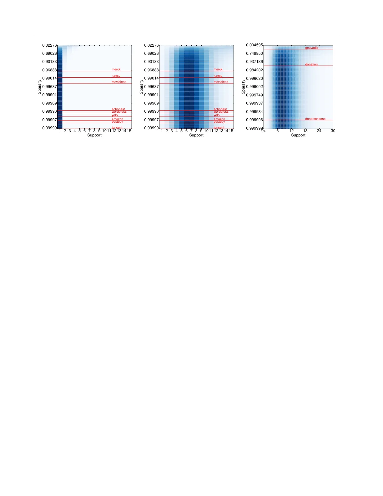
Hierar chical Compound P oisson F actorization Mehmet E. Basbug M E H M E T BA S B U G @ Y A H O O . C O M Princeton Univ ersity , 35 Olden St., Princeton, NJ 08540 USA Barbara E. Engelhardt B E E @ P R I N C E T O N . E D U Princeton Univ ersity , 35 Olden St., Princeton, NJ 08540 USA Abstract Non-negati v e matrix factorization models based on a hierarchical Gamma-Poisson structure cap- ture user and item behavior ef fecti v ely in e x- tremely sparse data sets, making them the ideal choice for collaborativ e filtering applications. Hierarchical Poisson factorization (HPF) in par- ticular has proved successful for scalable recom- mendation systems with e xtreme sparsity . HPF , howe v er , suffers from a tight coupling of spar- sity model (absence of a rating) and response model (the value of the rating), which limits the expressi veness of the latter . Here, we in- troduce hierarchical compound Poisson factor- ization (HCPF) that has the fa vorable Gamma- Poisson structure and scalability of HPF to high- dimensional extremely sparse matrices. More importantly , HCPF decouples the sparsity model from the response model, allowing us to choose the most suitable distribution for the response. HCPF can capture binary , non-negati ve discrete, non-negati ve continuous, and zero-inflated con- tinuous responses. W e compare HCPF with HPF on nine discrete and three continuous data sets and conclude that HCPF captures the relationship between sparsity and response better than HPF . 1. Introduction Matrix factorization has been a central subject in statis- tics since the introduction of principal component analy- sis (PCA) (Pearson, 1901). The goal is to embed data into a lower dimensional space with minimal loss of informa- tion. The dimensionality reduction aspect of matrix factor- ization has become increasingly important in exploratory data analysis as the dimensionality of data has exploded. Pr oceedings of the 33 rd International Confer ence on Machine Learning , New Y ork, NY , USA, 2016. JMLR: W&CP volume 48. Copyright 2016 by the author(s). One alternativ e to PCA, non-negati ve matrix factoriza- tion (NMF), was first dev eloped for factorizing matrices for face recognition (Lee & Seung, 1999). The idea be- hind NMF is that the contrib utions of each feature to a factor are non-negati ve. Although the motiv ation behind this choice has roots in cerebral representations of objects, non-negati veness has found great appeal in applications such as collaborativ e filtering (Gopalan et al., 2013), doc- ument classification (Xu et al., 2003), and signal process- ing (F ´ evotte et al., 2009). In collaborati ve filtering, the data are highly sparse user by item response matrices. For e xample, the Netflix movie rat- ing data set includes 480 K users, 17 K movies and 100 M ratings, meaning that 0 . 988 of the matrix entries are miss- ing. In the donors-choose data set, the user (donor) re- sponse to an item (project) quantifies their monetary dona- tion to that project; this matrix includes 1 . 3 M donors, 525 K projects and 2 . 66 M donations, meaning that 0 . 999996 of the matrix entries are missing. In the collaborati ve filtering literature, there are two school of thoughts on how to treat missing entries. The first one assumes that entries are missing at random; that is, we ob- serve a uniformly sampled subset of the data (Marlin et al., 2012). Factorization is done on the premise that the re- sponse v alue provides all the information needed. The sec- ond method assumes that matrix entries are not missing at random, but instead there is a underlying mixture model: first, a coin is flipped to determine if an entry is missing. If the entry is missing, its v alue is set to zero; if it is not miss- ing, the response is drawn from a specific distrib ution (Mar- lin & Zemel, 2009). In this frame work, we postulate that absence of an entry carries information about the item and the user , and this information can be exploited to improve the ov erall quality of the factorization. The dif ficult part is in representing the connection between the absence of a response (sparsity model) and the numerical value of a re- sponse (response model) (Little & Rubin, 2014). W e are concerned with the problem of sparse matrix factorization where the data are not missing at random. Hierarchical Compound P oisson Factorization Extensions to the NMF hint at a model that addresses this problem. Recent work showed that the NMF objec- tiv e function is equiv alent to a factorized Poisson likeli- hood (Cemgil, 2009). The authors proposed a Bayesian treatment of the Poisson model with Gamma conjugate pri- ors on the latent factors, laying the foundation for hierar- chical Poisson factorization (HPF) (Gopalan et al., 2013). The Gamma-Poisson structure is also used in earlier work for matrix factorization because of its fav orable behav- ior (Canny, 2004; Ma et al., 2011). Long tailed Gamma pri- ors were found to be powerful in capturing the underlying user and item behavior in collaborati ve filtering problems by applying strong shrinkage to the values near zero but allowing the non-zero responses to escape shrinkage (Pol- son & Scott, 2010). An extension of the Poisson factor- ization to non-discrete data using data augmentation has been considered (F ´ evotte et al., 2009; F ´ evotte & Idier, 2011). Along the similar lines, the connection between beta div ergences and compound Poisson Gamma distribu- tion is exploited to develop a non-negati ve matrix factoriza- tion model for sparse positive data (Simsekli et al., 2013). More recent work introduced a stochastic v ariational in- ference algorithm for scalable collaborativ e filtering using HPF (Gopalan et al., 2013). HPF models each factor contribution to be dra wn from a Poisson distribution with a long tail gamma prior . Thanks to the additiv e property of Poisson, the sum of these contri- butions are again a Poisson random v ariable which is used to model the response. For a collaborativ e filtering prob- lem, HPF treats missing entries as true zero responses when applied to both missing and non-missing entries (Gopalan et al., 2013). When the overwhelming majority of the ma- trix is missing, the posterior estimates for the Poisson fac- tors are close to zero. This mechanism has a profound im- pact on the response model: When the Poisson parameter of a zero truncated Poisson (ZTP) distribution approaches zero, the ZTP con verges to a degenerate distrib ution at 1 . In other words, if we condition on the fact that an entry is not missing, the HPF predicts that the response value is 1 with a very high probability . Since the response model and spar - sity model are so tightly coupled, HPF is suitable only for sparse binary matrices. When using HPF on the full matrix (i.e., missing data and responses together), one might bina- rize the data to improve performance of the HPF (Gopalan et al., 2013). Ho we ver , binarization ignores the impact of the response model on absence. For instance, a user is more likely to watch a movie that is similar to a movie that she gav e a high rating to relati ve to one that she rated lo wer . This information is ignored in the HPF model. In this paper , we introduce hierarchical compound Poisson factorization (HCPF), which has the same Gamma-Poisson structure as the HPF model and is equally computationally tractable. HCPF differs from the HPC in that it flexibility decouples the sparsity model from the response model, al- lowing the HCPF to accurately model binary , non-neg ative discrete, non-negati ve continuous and zero-inflated contin- uous responses in the context of extreme sparsity . Un- like HPF , the ZTP distrib ution does not concentrate around 1 , but instead con verges to the response distribution that we choose. In other words, we effecti vely decouple the sparsity model and the response model. Decoupling does not imply independence, but instead the ability to capture the distrib utional characteristics of the response more ac- curately in the presence of extreme sparsity . HCPF still retains the useful property of HPF that the expected non- missing response value is related to the probability of non- absence, allo wing the sparsity model to e xploit information from the responses. First we generalize HPF to handle non-discrete data. In Section 2, we introduce additive exponential dispersion models, a class of probability distributions. W e show that any member of the additi ve exponential dispersion model family , including normal, gamma, in verse Gaussian, Pois- son, binomial, negati ve binomial, and zero-truncated Pois- son, can be used for the response model. In Section 3, we prov e that a compound Poisson distribution con verges to its element additiv e EDM distribution as sparsity increases. Section 4 describes the generativ e model for hierarchical compound Poisson factorization (HCPF) and the mean field stochastic variational inference (SVI) algorithm for HCPF , which allows us to fit HCPF to data sets with millions of rows and columns quickly (Gopalan et al., 2013). In Sec- tion 5, we show the fav orable behavior of HCPF as com- pared to HPF on twelve data sets of v arying size including ratings data sets ( amazon, movielens, netflix and yelp ), so- cial media activity data sets ( wordpr ess and tencent ), a web activity data set ( bestbuy ), a music data set ( echonest ), a biochemistry data set ( merc k ), financial data sets ( donation and donorschoose ), and a genomics data set ( g euvadis ). 2. Exponential Dispersion Models Additiv e exponential dispersion models (EDMs) are a gen- eralization of the natural exponential family where the nonzero dispersion parameter scales the log-partition func- tion (Jorgensen, 1997). W e first giv e a formal definition of additiv e EDM, and present sev en useful members (T able 1). Definition 1. A family of distributions F Ψ =  p (Ψ ,θ,κ ) | θ ∈ Θ = dom (Ψ) ⊆ R , κ ∈ R ++  is called an additiv e exponential dispersion model if p (Ψ ,θ,κ ) ( x ) = exp( xθ − κ Ψ( θ )) h ( x, κ ) (1) wher e θ is the natural parameter , κ is the dispersion param- eter , Ψ( θ ) is the base log-partition function, and h ( x, κ ) is the base measur e. Hierarchical Compound P oisson Factorization T able 1. Seven common additiv e exponential dispersion models. Normal, gamma, in verse Gaussian, Poisson, binomial, negati ve binomial, and zero truncated Poisson (ZTP) distributions written in additive EDM form with the variational distribution of the Poisson variable for the corresponding compound Poisson additi ve EDM. The gamma distrib ution is parametrized with shape ( a ) and rate ( b ). D I S T RI B U T I O N θ κ Ψ( θ ) h ( x, κ ) q ( n ui = n ) ∝ N O R M AL N ( µ, σ 2 ) µ σ 2 σ 2 θ 2 2 1 √ 2 πκ exp( − x 2 2 κ ) exp n − n 2 µ 2 + y 2 ui 2 nσ 2 o Λ n ui n ! √ n G A M M A Ga ( a, b ) − b a − log( − θ ) x κ − 1 / Γ( κ ) ( b a y a ui Λ ui ) n Γ( na ) n ! I N V . G AU S S I A N I G ( µ, λ ) − λ 2 µ 2 √ λ − √ − 2 θ κ √ 2 πx 3 exp( − κ 2 2 x ) exp n n λ µ − n 2 λ 2 y ui o Λ n ui ( n − 1)! P O I S SO N P o ( λ ) log λ 1 e θ κ x x ! exp {− nλ } n y ui Λ n ui n ! B I N O M IA L B i ( r , p ) log p 1 − p r log(1 + e θ )  κ x  ( nr )!(1 − p ) nr Λ n ui n !( nr − y ui )! N E G . B I N O M I A L N B ( r , p ) log p r − log(1 − e θ )  x + κ − 1 x  ( y ui + nr − 1)!(1 − p ) nr Λ n ui n !( nr − 1)! Z T P Z T P ( λ ) log λ 1 log( e e θ − 1) 1 x ! P κ j =0 ( − 1) j ( κ − j ) x  κ j   Λ ui e λ − 1  n P n j =0 ( − 1) j ( n − j ) y ui j !( n − j )! The sum of additi ve EDMs with a shared natural parameter and base log partition function is again an additi ve EDM of the same type. Theorem 1 (Jor gensen, 1997) . Let X 1 . . . X M be a se- quence of additive EDMs such that X i ∼ p Ψ ( x ; θ , κ i ) , then X + = X 1 + · · · + X M ∼ p Ψ ( x ; θ , P i κ i ) . In T able 1, we use a generalized definition of the zero truncated Poisson (ZTP) where the density of the sum of κ i.i.d. random v ariables from an ordinary ZTP distribu- tion can be expressed with the same formula (Springael & V an Nieuwenhuyse, 2006). The last column in T able 1 shows the variational update for the Poisson parameter of the compound Poisson additive EDM, further discussed in Section 3. 3. Compound Poisson Distrib utions W e start with the general definition of a compound Poisson distribution and discuss compound Poisson additive EDM distributions. W e then present the decoupling theorem and explain the implications of the theorem in detail. Definition 2. Let N be a P oisson distributed random vari- able with parameter Λ , X 1 , . . . , X N be i.i.d. random vari- ables distributed with an element distribution p Ψ ( x ; θ , κ ) . Then X + . = X 1 + · · · + X N ∼ p Ψ ( x ; θ , κ, Λ) is called a compound Poisson random variable . In general, p Ψ ( x ; θ , κ, Λ) does not have a closed form ex- pression, but it is a well defined probability distribution. The conditional form, X + | N , is usually easier to manip- ulate, and we can calculate the mar ginal distrib ution of X + by integrating out N . When N = 0 , X + has a degenerate distribution at zero. Furthermore, if the element distribu- tion is an additiv e EDM, we have the follo wing theorem: Theorem 2. Let X ∼ p Ψ ( x ; θ , κ ) be an additive EDM and X + ∼ p Ψ ( x ; θ , κ, Λ) be the compound P oisson random variable with the element random variable X , then X + | N = n ∼ p Ψ ( x ; θ , nκ ) (2) X + | N = 0 ∼ δ 0 . (3) Theorem 2 implies that the conditional distribution of a compound Poisson additi ve EDM is again an additiv e EDM. Hence, both the conditional and the marginal den- sities of X + can be calculated easily . W e make the following remark before the decoupling the- orem. Later, we sho w that HPF is a degenerate form of our model using this remark. Remark 1. Compound P oisson r andom variable X + is an or dinary P oisson r andom variable with par ameter Λ if and only if the element distribution is a de gener ate distribution at 1 . W e now present the decoupling theorem. This theorem shows that the distrib ution of a zero truncated compound Poisson random variable con verges to its element distribu- tion as the Poisson parameter ( Λ ) goes to zero. Theorem 3. Let X ++ . = X + | X + 6 = 0 be a zer o truncated compound P oisson random variable with element random variable X . If zer o is not in the support of X , then P r ( X + = 0) = e − Λ (4) E [ X ++ ] = Λ 1 − e − Λ E [ X ] (5) X ++ D → X as Λ → 0 . (6) Hierarchical Compound P oisson Factorization 1 2 3 4 5 6 7 8 9 10 11 12 13 14 15 Suppor t 0.99999 0.99997 0.99990 0.99969 0.99901 0.99687 0.99014 0.96888 0.90183 0.69026 0.02276 Sparsity y elp netflix bestb uy mo vielens amaz on merc k w ordpress tencent echonest (a) 1 2 3 4 5 6 7 8 9 10 11 12 13 14 15 Suppor t 0.99999 0.99997 0.99990 0.99969 0.99901 0.99687 0.99014 0.96888 0.90183 0.69026 0.02276 Sparsity y elp netflix bestb uy mo vielens amaz on merc k w ordpress tencent echonest (b) 0+ 6 12 18 24 30 Suppor t 0.999999 0.999996 0.999984 0.999937 0.999749 0.999002 0.996030 0.984202 0.937136 0.749850 0.004595 Sparsity donation donorschoose geuv adis (c) Figure 1. PDF of the zero truncated compound Poisson random variable X ++ at various sparsity levels on log scale. The PDF is color coded, where darker colors correspond to greater density . The response distribution is a) a degenerate δ 1 , b) a zero truncated Poisson with λ = 7 , c) a gamma distribution with a = 5 , b = 0 . 5 . Red vertical lines mark the sparsity le vels of various data sets. Proofs of Theorem 2, 3 and Remark 1 can be found in the Appendix. Let X + be a compound Poisson variable with element ran- dom distribution p Ψ ( x ; θ , κ ) and let X ++ be the zero trun- cated X + as in Theorem 3. W e can study the probability density function (PDF) of X ++ at v arious sparsity lev els (Fig 1; Eq 4) with respect to the average sparsity levels of our 9 discrete data sets and 3 continuous data sets. Impor- tantly , the element distrib ution is nearly identical across all lev els of sparsity . W e will use X + to model an entry of a full sparse ma- trix, meaning that we are including both missing and non- missing entries. The zero truncated random v ariable, X ++ , corresponds to the non-missing response. In Fig 1a, X + is an ordinary Poisson v ariable. As Remark 1 and Theorem 3 suggest, at levels of extreme sparsity (i.e., > 90% zeros), almost all of the probability mass of X ++ concentrates at 1 . That is, HPF predicts that, if an entry is not missing, then its v alue is 1 with a high probability . T o get a more fle xible response model, we might regularize X + with appropriate gamma priors; howe ver , this approach would degrade the performance of the sparsity model. On the other hand, when X + is a compound Poisson- ZTP random v ariable with λ = 7 , e xtreme sparsity lev- els have virtually no effect on the distribution of the re- sponse (Fig 1b). Using the HCPF , we are free to choose any additive distribution for the response model. For dis- crete response data, we might opt for degenerate, Poisson, binomial, negati ve binomial or ZTP and for continuous re- sponse data, we might select gamma, in verse Gaussian or normal distribution. Furthermore, HCPF explicitly encodes a relationship between non-absence, P r ( X + 6 = 0) , and the expected non-missing response v alue, E [ X ++ ] (Eq 4 and Eq 5), which is defined via the choice of response model. HPF , as a degenerate HCPF model, defines this relation- ship as X ∼ δ 1 and E [ X ++ ] = 1 , which leads to the poor behavior outside of binary sparse matrices. Along with the flexibility of choosing the most natural element distribu- tion, HCPF is capable of decoupling the sparsity and re- sponse models while still encoding a data-specific relation- ship between the sparsity model and the values of the non- zero responses in expectation. 4. Hierarchical Compound P oisson F actorization (HCPF) Next, we describe the generativ e process for HCPF and the Gamma-Poisson structure. W e explain the intuition be- hind the choices of the long-tailed Gamma priors. W e then present the stochastic variational inference (SVI) algorithm for HCPF . W e can write the generati ve model of the HCPF with ele- ment distribution p Ψ ( x ; θ , κ ) with fix ed hyperparameters θ and κ as follo ws, where C U and C I are the number of users and items, respectiv ely: • For each user u = 1 , . . . , C U 1. Sample r u ∼ Ga ( ρ, ρ/% ) 2. For each component k , sample s uk ∼ Ga ( η , r u ) • For each item i = 1 , . . . , C I 1. Sample w i ∼ Ga ( ω , ω /$ ) 2. For each component k , sample v ik ∼ Ga ( ζ , w i ) • For each user u and item i 1. Sample count n ui ∼ P o ( P k s uk v ik ) 2. Sample response y ui ∼ p Ψ ( θ , n ui κ ) Hierarchical Compound P oisson Factorization Algorithm 1 SVI for HCPF Initialize: Hyperparameters η , ζ , ρ, %, ω , $ , θ, κ, τ , ξ and parameters t u = τ , t i = τ , b r u = ρ/%, a s uk = η b s uk = %, b w i = ω /$, a v ik = ζ , b v ik = $ Fix: a r u = ρ + K η a w i = ω + K ζ repeat Sample an observation y ui uniformly from the data set Compute local variational parameters Λ ui = X k a s uk a v ik b s uk b v ik q ( n ui = n ) ∝ exp {− κn Ψ( θ ) } h ( y ui , nκ ) Λ n ui n ! ϕ uik ∝ exp { Ψ( a s uk ) − log b s uk +Ψ( a v ik ) − log b v ik } Update global variational parameters b r u = (1 − t − ξ u ) b r u + t − ξ u ρ % + X k a s uk b s uk ! a s uk = (1 − t − ξ u ) a s uk + t − ξ u ( η + C I E [ n ui ] ϕ uik ) b s uk = (1 − t − ξ u ) b s uk + t − ξ u  a r u b r u + C I a v ik b v ik  b w i = (1 − t − ξ i ) b w i + t − ξ i ω $ + X k a v ik b v ik ! a v ik = (1 − t − ξ i ) a v ik + t − ξ i ( ζ + C U E [ n ui ] ϕ uik ) b v ik = (1 − t − ξ i ) b v ik + t − ξ i  a w i b w i + C U a s uk b s uk  Update learning rates t u = t u + 1 t i = t i + 1 (Optional) Update hyperparameters θ and κ until V alidation log likelihood con ver ges The mean field variational distribution for HCPF is gi ven by q ( r u | a r u , b r u ) q ( s uk | a s uk , b s uk ) q ( w i | a w i , b w i ) q ( v ik | a v ik , b v ik ) q ( z ui | ϕ ui ) q ( n ui ) . The choice of long tail g amma priors has substantial impli- cations for the response model in a collaborativ e filtering framew ork.The effect of the gamma prior on a particular user’ s responses is to effect iv ely characterize her av erage response. Similarly , a gamma prior on a particular item models the average users’ response for that item. The long tail gamma prior assumption for users allows some users to have unusually high responses. For instance, in the do- nations data, we might expect to observe a few donors who make extraordinarily large donations to a few projects. This is not appropriate for movie ratings, since the maximum rating is 5 , and a substantial number of non-missing ratings are fi ves. The long tail gamma prior for items allow a fe w items to recei ve unusually high av erage responses. This is a useful property of all of our data sets: we imagine that a few projects may attract particularly lar ge donations, a few blogs may recei ve a lot of lik es , or a few movies recei ve an unusually high av erage rating. The choice of long tail gamma priors has different implica- tions in terms of the sparsity model. The gamma prior on a particular user models ho w active she is, that is, how man y items she has responses for . The long tail assumption on the sparsity model implies that there are unusually activ e users (e.g., cinephiles or frequent donors). The long tail as- sumption for items corresponds to very popular items with a large number of responses. Note that the mo vies with the most ratings are not necessarily the highest rated movies. W e lev erage the fact that the contributions of Poisson fac- tors can be written as a multinomial distrib ution (Cemgil, 2009). Using this, we can write out the stochastic vari- ational inference algorithm for HCPF (Hoffman et al., 2013), where τ and ξ are the learning rate delay and learn- ing rate power , and τ > 0 and 0 . 5 < ξ < 1 . 0 (Alg 1). Note that the HCPF is not a conjugate model due to q ( n ui ) . For other variational updates, we only need the statistics E [ n ui ] . For that purpose, we calculate q ( n ui = n ) ex- plicitly for n = 1 , . . . , N tr . The choice for the truncation value, N tr , depends on θ, κ , and Λ ui . W e set N tr using the expected range of Λ ui and y ui as well as fixed θ and κ . HCPF reduces to HPF when we set q ( n ui ) = δ y ui . The specific form of q ( n ui ) for different additiv e EDMs is giv en in T able 1. 5. Results 5.1. Data sets for collaborati ve filtering W e performed matrix factorization on 12 different data sets with dif ferent le vels of sparsity , response character- istics, and sizes (T able 2). The rating data sets include amazon fine food ratings (McAuley & Leskov ec, 2013), movielens (Harper & K onstan, 2015), netflix (Bell & K o- ren, 2007) and yelp , where the responses are a star rating from 1 to 5 . The only exception is movielens where the maximum rating is 10 . The social media data sets include wor dpress and tencent (Niu et al., 2012), where the re- sponse is the number of likes, a non-negati ve integer v alue. Commercial data sets include bestb uy , where the response is the number of user visit to a product page. The biochem- Hierarchical Compound P oisson Factorization istry data sets include mer ck (Ma et al., 2015), which cap- tures molecules (users) and chemical characteristics (items) where the response is the chemical acti vity . In echon- est (Bertin-Mahieux et al., 2011), the response is the num- ber of times a user listened a song. The donation data sets donation and donorschoose includes donors and projects, where the response is the total amount of a donation in US dollars. The genomics data set geuvadis includes genes and individuals, where the response is the gene expression lev el for a user of a gene (Lappalainen et al., 2013). Both best- buy and mer ck are nearly binary matrices, meaning that the vast majority of the non-missing entries are one. On the other hand, donation , donorschoose , and geuvadis hav e a continuous response variable. 5.2. Experimental setup W e held out 20% and 1% of the non-missing entries for testing ( Y test N M ) and v alidation, respectiv ely . W e also sam- pled an equal number of missing entries for testing ( Y test M ) and validation. When calculating test and validation log likelihood, the log likelihood of the missing entries is ad- justed to reflect the true sparsity ratio. T est log likelihood of the missing ( L M ) and non-missing entries ( L N M ) as well as the test log likelihood of a non-missing entry conditioned on that it is not missing ( L C N M ) are calculated as L M = X Y test M log P o ( n = 0 | Λ ui ) L N M = X Y test N M log N tr X n =0 p Ψ ( y test ui ; θ , nκ ) P o ( n | Λ ui ) L = 0 . 2(# total missing ) | Y test M | L M + L N M L C N M = X Y test N M log N tr X n =1 p Ψ ( y test ui ; θ , nκ ) Z T P ( n | Λ ui ) . In HCPF , we fix K = 160 , ξ = 0 . 7 and τ = 10 , 000 after an empirical study on smaller data sets. T o set hyper- parameters θ and κ , we use the maximum likelihood esti- mates of the element distribution parameters on the non- missing entries. From the number of non-missing entries in the training data set, we inferred the sparsity level, ef- fectiv ely estimating E [ n ui ] empirically (note that we as- sume E [ n ui ] is the same for e very user-item pair). W e then used E [ n ui ] to set the factorization hyperparameters η , ζ , ρ, %, ω , $ . T o create hea vy tails and uninformativ e gamma priors, we set $ = % = 0 . 1 and ω = ρ = 0 . 01 . W e then assumed that the contribution of each factor is equal, and set η = % p E [ n ui ] /K and ζ = $ p E [ n ui ] /K . When training on the non-missing entries only , we simply assume that the sparsity le vel is very lo w ( 0 . 001 ), and from that we set the parameters as usual, and divide the maximum like- T able 2. Data set characteristics Number of rows, columns, non- missing entries, and the ratio of missing entries to the total number of entries (sparsity) for the data sets we analyzed. DAT A S E T # R OW S # C O LS S P A R S IT Y # N ON - M IS S IN G A MA Z ON 2 5 6, 0 59 74 , 25 8 0 .9 9 9 97 0 5 68 , 4 54 M OV IE L EN S 1 3 8 ,4 9 3 2 6 , 74 4 0 . 9 94 6 00 2 0 ,0 0 0 ,2 6 3 N ET FL IX 4 80 , 1 89 1 7, 7 7 0 0 .9 8 8 22 4 1 00 , 4 83 , 02 4 Y EL P 5 52 , 3 39 7 7, 0 7 9 0 .9 9 9 94 7 2 ,2 2 5 ,2 1 3 W OR D PR E SS 8 6, 6 61 7 8 ,7 5 4 0 . 99 9 91 5 5 8 1, 5 08 T EN C EN T 1 , 3 58 , 84 2 8 78 , 70 8 0 .9 9 99 9 1 1 0, 6 18 , 5 84 B ES T BU Y 1 , 2 68 , 70 2 6 9, 8 58 0 . 99 9 97 9 1 , 86 2 ,7 8 2 M ER C K 1 52 , 9 35 1 0, 8 8 3 0 .9 7 0 52 4 4 9, 0 59 , 3 40 E CH O NE S T 1 ,0 1 9 ,3 1 8 3 8 4, 5 46 0 . 99 9 87 7 4 8 ,3 7 3, 5 86 D ON A T I ON 3 94 , 2 66 8 2 0 .9 6 58 3 1 1 ,1 0 4, 6 8 7 D CH O OS E 1, 2 8 2, 0 62 5 2 5, 0 19 0 . 99 9 9 96 2 , 66 1 , 82 0 G EU V A D IS 9 ,3 5 8 4 62 0 . 46 2 12 2 2 , 32 5 ,4 6 1 lihood estimate of κ by E [ n ui ] . Earlier work noted that HPF is not sensitiv e to hyperparameter settings within rea- son (Gopalan et al., 2013). T o identify the best response model for HCPF , we ran SVI with all sev en additi ve EDM distributions in T able 1. W e first fit all HCPF models by sampling from the full matrix. W e calculated L , L M , L N M and L C N M . In Section 5.3, we compare HCPF and HPF in L . In the second analysis, we only used the non-missing entries for training and cal- culated L N M . In Section 5.4, we compared L C N M of the first analysis to L N M of the second analysis. 5.3. Overall perf ormance In this analysis we quantify ho w well these models capture both the sparsity and response behavior in ultra sparse ma- trices. In a movie ratings data set, the question becomes ‘Can we predict if a user would rate a gi ven movie and if she does what rating she would give?’. W e report the test log likelihood of all twelve data sets. W e fit HCPF with nor- mal, gamma, and in verse Gaussian as element distrib utions for all the data sets. In discrete data sets, we additionally fit HPF and HCPF with Poisson, binomial, ne gativ e binomial, and zero truncated Poisson element distributions. In all ratings data sets ( amazon, movielens, netflix , and yelp ), HCPF significantly outperforms HPF (T able 3). The relativ e performance dif ference is ev en more pronounced in sparser data sets ( amazon and yelp ). When we break down the test log likelihood into missing and non-missing parts, we see that, in sparser data sets, the relativ e perfor- mance of HPF for non-missing entries is much weaker than it is for less sparse data sets. This is expected, as response coupling in HPF is stronger in sparser data sets, forcing the response variables to zero. The opposite is true for HCPF: its performance improv es with increasing data sparsity . In social media acti vity data ( wordpr ess and tencent ) and the music data set ( echonest ), HCPF shows a significant improv ement over HPF (T able 3). Unlike the ratings data sets, we hav e an unbounded response v ariable with an ex- Hierarchical Compound P oisson Factorization T able 3. T est log likelihood. Per-thousand-entry test log likelihood for HCPF and HPF trained on the full matrix for twelve data sets. Discrete HCPF models and HPF are not applicable to continuous data sets (N/A). Element distribution acron yms in T able 1. A MA Z ON M OV IE L EN S N ET FL IX Y EL P W OR D PR E SS T EN C EN T E CH O NE S T B ES T BU Y M ER C K D ON A T I ON D CH O OS E G EU V A D IS H CP F - N -0 . 38 8 - 27 . 4 80 - 5 0. 4 61 -0.625 - 0 .9 0 9 - 0 .1 4 8 - 1 .5 0 2 - 0 .2 3 1 - 1 29 . 22 5 - 28 4 .1 7 8 - 0 .1 0 0 -4 4 24 . 2 88 H CP F - GA - 0 . 40 2 - 2 8 .5 4 6 - 5 1. 5 58 - 0 .6 4 8 -0.804 -0.129 - 1. 6 9 7 - 0. 2 2 1 - 10 7 . 56 9 - 2 6 0. 7 04 -0.095 -2527.897 H CP F - IG - 0 . 40 1 - 2 7 .7 6 4 - 5 1. 1 52 - 0 .6 5 7 - 0 .8 7 6 -0.129 - 1 .6 4 8 -0.215 - 9 3 .9 8 9 -254.055 -0.095 -3 6 3 27 . 64 4 H CP F - PO - 0. 3 9 2 -27.056 - 51 . 3 32 - 0. 6 3 6 - 0. 8 7 2 - 0. 1 8 3 -1.447 - 0. 2 98 - 1 36 . 6 09 N /A N / A N /A H CP F - BI -0.387 -2 7 . 78 1 -50.152 - 0 . 70 8 - 0 . 93 0 - 0 . 17 4 - 1 . 87 1 - 0 . 28 9 - 1 1 6. 8 86 N / A N / A N / A H CP F - NB - 0. 4 0 4 - 28 . 8 86 - 55 . 2 01 - 0 .7 0 1 - 0 .8 1 8 - 0 .1 4 3 - 1 .7 0 9 - 0 .3 4 2 - 1 11 . 61 3 N /A N /A N /A H CP F - ZT P - 0 . 38 9 - 2 7 .9 3 2 - 5 2. 6 98 - 0 .6 6 1 - 0 .8 5 0 - 0 .1 7 0 - 1 .8 4 6 - 0 .3 0 4 - 1 13 . 85 6 N /A N /A N /A H PF - 1. 4 5 3 - 76 . 1 82 - 88 . 4 90 - 2 .0 2 6 - 1 .3 7 8 - 0 .5 8 3 - 3 .2 4 6 - 0 .2 8 9 -86.492 N /A N / A N /A T able 4. Non-missing test log likelihood. Per non-missing entry test log likelihood of HCPF and HPF trained on the full matrix and on the non-missing entries only (marked as ‘F’ and ‘NM, ’ respectively). When trained on the full matrix, the conditional non-missing test log likelihood is reported. A MA Z ON M OV IE L EN S N ET FL IX Y EL P W OR D PR E SS T EN C EN T E CH O NE S T B ES T BU Y M ER C K D ON A T I ON D CH O OS E G EU V A D IS H CP F - N F - 1 .6 9 2 - 2 .2 9 0 - 1 .6 4 2 -1 . 73 4 - 3. 0 2 6 - 4 .3 9 1 -3 . 20 1 - 0. 8 72 - 2 .8 5 5 - 4 .9 8 5 - 6 .8 0 6 -6 . 84 1 N M - 6 . 30 2 - 2 . 26 8 - 1 . 61 7 -3 . 5 73 - 2 .8 6 0 - 3 . 93 3 -2 . 7 06 - 1 6. 7 54 - 2 .4 0 3 - 4 .8 8 1 - 7 .4 2 1 - 7 . 17 3 H CP F - GA F -1 . 9 09 - 2 .4 1 7 - 1 .7 0 8 - 1 . 87 6 - 1 . 75 4 -2 . 5 00 - 2. 0 4 9 - 0 .8 3 5 - 2 .1 5 1 - 4 .3 3 8 - 5 .3 8 7 -3.341 N M - 4 . 10 2 - 2 . 31 0 - 1 . 64 9 -2 . 7 76 - 2 .2 3 4 - 2 . 76 1 -2 . 0 53 - 1 7. 2 65 - 2 .0 7 9 - 4 .2 1 3 - 6 .9 0 6 - 4 . 12 9 H CP F - IG F - 2. 0 77 - 2 .3 6 3 - 1 .6 6 5 -1 . 99 9 -1.440 -2.040 -1.752 - 0 .7 8 2 - 1 .6 8 5 -4.132 -5.340 - 66 . 2 28 N M - 5 . 96 5 - 2 . 69 0 - 3 . 41 9 -5 . 5 89 - 7 .0 1 7 - 7 . 47 0 -6 . 9 79 - 8. 2 4 7 - 7. 4 7 4 - 7. 1 3 5 - 6. 1 5 5 - 10 . 1 21 H CP F - PO F - 1. 8 7 7 - 2. 2 5 5 - 1. 7 5 6 - 1 .8 5 6 - 2 .4 4 8 -7 . 96 0 - 3. 0 17 - 1 .0 0 1 - 3 .1 8 6 N /A N / A N /A N M - 7 . 20 6 - 9 . 81 9 - 5 . 60 8 -6 . 2 10 - 5 .2 3 4 - 1 2. 6 33 - 6 .1 4 5 - 3 . 17 5 - 6 . 67 3 N / A N /A N/ A H CP F - BI F -1.559 - 2 . 20 8 -1.586 -1.704 - 2. 4 4 9 - 6 .9 1 1 -3 . 08 5 - 0. 6 94 - 2 .4 5 7 N / A N / A N / A N M - 2 . 11 3 - 2 . 21 4 - 1 . 62 6 -1 . 8 41 - 2 .6 4 9 - 5 . 48 0 -2 . 4 48 - 1. 1 0 2 - 1. 9 9 3 N / A N / A N /A H CP F - NB F - 2. 1 1 3 - 2. 5 1 0 - 2. 0 7 8 - 2 .0 6 7 - 1 .9 5 8 -3 . 44 1 - 2. 2 72 - 1 .3 4 9 - 2 .2 6 7 N /A N / A N /A N M - 3 . 77 2 - 2 . 52 6 - 2 . 08 2 -2 . 7 93 - 2 .3 4 4 - 3 . 27 2 -2 . 1 78 - 3. 1 0 4 - 2. 0 8 5 N / A N / A N /A H CP F - ZT P F - 1 . 86 5 - 2 . 35 6 - 1 . 82 1 -1 . 8 32 - 2. 2 8 3 - 6 .9 2 4 -3 . 00 8 -0.010 - 2 . 32 3 N / A N / A N / A N M - 6 . 85 3 - 5 . 32 4 - 5 . 54 1 -5 . 7 41 - 5 .4 0 6 - 1 2. 1 23 - 5 .9 5 2 - 3 . 00 2 - 6 . 65 3 N / A N /A N/ A H PF F - 35 . 6 66 - 9. 7 0 3 - 4. 6 2 3 - 27 . 0 25 - 7 .1 6 7 - 6 3. 7 94 - 2 2. 8 95 - 0 .0 1 7 -1.535 N / A N / A N /A N M - 1 . 86 8 -2.095 - 1 . 67 2 -1 . 9 40 - 2. 5 2 2 - 6 .7 8 4 -2 . 64 0 - 3. 3 05 - 1 .5 6 3 N / A N / A N / A ponentially decaying characteristic. At first HPF might seem to be a good model for such data; howev er , the spar- sity level is so high that the non-missing point mass con- centrates at 1 . This is best seen in the comparison of HPF with HCPF-ZTP . Although the Poisson distribution seems to capture response characteristic ef fectively , the test per - formance degrades when zero is included as part of the re- sponse model (as in HPF). In the bestb uy and merc k data sets, where the response is near binary , HPF and HCPF performances are very simi- lar . This confirms the observ ation that HPF is a sufficiently good model for sparse binary data sets. In the financial data sets ( donation and donors-choose ), we see that the gamma and in verse Gaussian are better distributional choices than the normal as the element distribution. 5.4. Response model evaluated using test log lik elihood In this section, we in vestigate which model captures the response most accurately . In a movie ratings data set, the question becomes ‘Can we predict what rating a user would giv e to a movie gi ven that we kno w she rated that movie?’. In T able 4, we report the conditional non-missing test log likelihood of models trained on the full matrix and test log likelihood of the models trained only on the non-missing entries. First, we note that training HPF only on the non-missing entries results in a better response model than training HPF on the full matrix. The only exception is bestbuy where the conditional non-missing test log likelihood is near per- fect. This is due to the near binary structure of the data set. When we kno w if an entry is not missing, then we are f airly confident that it has a value of 1 . Secondly , we inv estigate if modeling the missing entries explicitly helps the response model. W e compare HPF trained on the non-missing entries to HCPF trained on the full matrix. HCPF-BI outperforms HPF in all ratings data sets except for movielens . A similar pattern can be seen in social media and music data sets where HCPF-IG seems to Hierarchical Compound P oisson Factorization T able 5. T est A UC T est A UC values for HCPF trained on the full matrix and HPF trained on the binarized full matrix. A MA Z ON M OV IE L EN S N ET FL IX Y EL P W OR D PR E SS T EN C EN T E CH O NE S T B ES T BU Y M ER C K D ON A T I ON D CH O OS E G EU V A D IS H CP F - N F 0 .8 0 2 0 0 .9 8 5 4 0 .9 7 2 0 0.8768 0 .8 9 91 0 . 91 6 7 0 . 91 1 1 0 . 88 9 2 0 . 98 7 2 0.8804 0 . 60 0 2 0 . 77 4 9 H CP F - GA F 0 . 79 8 6 0 . 98 3 9 0 . 97 2 3 0 . 86 5 1 0 . 89 4 3 0 . 91 7 5 0 . 89 1 2 0.8893 0 .9 8 8 0 0 .8 7 7 5 0 .6 5 4 3 0 .7 7 4 0 H CP F - IG F 0 . 80 1 7 0 . 98 5 6 0 . 97 2 2 0 . 86 8 1 0 . 89 5 3 0 . 91 3 6 0 . 88 9 2 0 . 88 3 0 0 . 98 8 0 0 . 87 7 3 0 . 59 6 7 0 . 77 3 3 H CP F - PO F 0.8034 0.9860 0 . 97 2 1 0 . 87 3 1 0 . 89 8 9 0 . 91 1 0 0.9124 0 . 88 5 9 0 . 98 8 4 N / A N /A N/ A H CP F - BI F 0 . 80 0 4 0 . 98 4 8 0 . 97 2 5 0 . 84 5 2 0 . 89 8 5 0 . 91 6 4 0 . 89 3 2 0 . 88 7 8 0.9885 N /A N/ A N /A H CP F - NB F 0. 7 9 89 0 . 98 4 4 0.9729 0 .8 5 1 0 0.9002 0 .9 1 19 0 . 89 0 8 0 . 81 6 8 0 . 98 7 7 N / A N / A N /A H CP F - ZT P F 0 . 80 2 5 0 . 98 4 9 0 . 97 1 7 0 . 86 4 0 0 . 89 9 9 0.9176 0 .8 9 2 2 0 .8 4 4 0 0 .9 8 7 6 N /A N / A N / A H PF B 0 . 8 02 1 0 . 9 85 5 0 . 9 71 8 0 . 8 50 8 0 . 8 97 1 0 . 9 14 6 0 . 8 90 1 0 . 8 86 0 0 . 9 87 9 0 . 8 78 0 0.6552 0.7769 be the best model. This phenomenon can be attributed to better identification of the relationship between the sparsity model and the re- sponse model. Although HPF trained on the full matrix can also capture this relationship, the high sparsity le vels force HPF to fit near-zero Poisson parameters, hurting the prediction for response. In ratings data sets, HCPF cap- tures the notion that more likely people are to consume an item, higher their responses are. In movielens and netflix for instance, we know that the most watched movies tend to have higher ratings. In social media data sets, the re- lation between the reach and popularity is captured. The more followers a blog has, the more content it is likely to produce, and the more reaction it will get. A similar cor- relation exists for the users as well. The more activ e users are also the more responsiv e ones. In summary , HCPF can capture the relationship between the non-missingness of an entry and the actual value of the entry if it is non-missing. Any NMF algorithm that makes the missing at random as- sumption would miss this relationship. One might ar gue that perhaps HPF is not a good model be- cause the underlying response distribution is not Possion like. Comparing the ro ws marked ‘NM’, we observe that there is some truth to this ar gument. In netflix and yelp data sets, HCPF-BI outperforms HPF; howe ver , we also see that training HCPF-BI on the full matrix is even better . A sim- ilar argument can be made for HCPF-GA in social media data sets ( wor dpr ess and tencent ). The flexibility of HCPF is a key factor to identifying the underlying response dis- tribution. The ability to model sparsity and response at the same time gives HCPF a further edge in modeling response. 5.5. Sparsity model evaluated using A UC In a movie ratings data set or a purchasing data set, one important question is ‘Can we predict if a user would rate a giv en movie or b uy a certain item?’. T o understand the quality of our performance on this task, we ev aluated the sparsity model separately by computing the area under the R OC curve (A UC), fitting all HCPF models by sampling from the full matrix and HPF to the binarized full matrix (T able 5). T o calculate the A UC, the true label is whether the data are missing ( 0 ) or non-missing ( 1 ), and we used the estimated probability of a non-missing entry , P r ( X + 6 = 0) , as the model prediction. As discussed in Section 5.3, when we fit HPF to the full matrix, we compromise performance on sparsity and response. HCPF , on the other hand, enjoys the decoupling effect while preserving the relationship in expectation (see Eq 5). In 10 of the 12 data sets, we get an improv ement ov er HPF (T able 5); this is somewhat surpris- ing as the HPF is specialized to this task; this illustrates the benefit of coupling the sparsity and response models in e x- pectation. Better modeling of the response w ould naturally lead to a better sparsity model. 6. Conclusion In this paper , we first proved that a zero truncated com- pound Poisson distribution con verges to its element distri- bution as sparsity increases. The implication of this the- orem for HPF is that the non-missing response distribu- tion concentrates at 1 , which is not a good response model unless we ha ve a binary data set. Inspired by the con ver - gence theorem, we introduce HCPF . Similar to HPF , HCPF has the fa vorable Gamma-Poisson structure to model long- tailed user and item activity . Unlike HPF , HCPF is capa- ble of modeling binary , non-negati ve discrete, non-negativ e continuous and zero-inflated continuous data. More impor - tantly , HCPF decouples the sparsity and response models, allowing us to specify the most suitable distrib ution for the non-missing response entries. W e sho w that this decou- pling effect improv es the test log likelihood dramatically when compared to HPF on high-dimensional, extremely sparse matrices. HCPF also shows superior performance to HPF trained exclusi vely on non-missing entries in terms of modeling response. Finally , we show that HCPF is a better sparsity model than HPF , despite HPF tar geting this sparsity behavior . For future directions, we will in vestigate the implications of the decoupling theorem in other Bayesian settings. W e will also explore hierarchical latent structures for the element distribution. Hierarchical Compound P oisson Factorization Acknowledgements BEE was funded by NIH R00 HG006265, NIH R01 MH101822, and a Sloan Faculty Fellowship. MEB was funded in part by the Princeton Innovation J. Insley Blair Pyne Fund A ward. W e would like to thank Robert E. Schapire for valuable discussions. References Bell, R. M. and Koren, Y . Lessons from the netflix prize challenge. ACM SIGKDD Explorations Newslet- ter , 2007. Bertin-Mahieux, T ., Ellis, D. P . W ., Whitman, B., and Lamere, P . The million song dataset. In International So- ciety for Music Information Retrieval Confer ence , 2011. Canny , J. Gap: a factor model for discrete data. In ACM SIGIR Confer ence on Resear ch and Development in In- formation Retrieval , 2004. Cemgil, A. T . Bayesian inference for nonnegati ve matrix factorisation models. Computational Intelligence and Neur oscience , 2009. F ´ evotte, C. and Idier , J. Algorithms for nonnegati ve matrix factorization with the β -div ergence. Neural Computa- tion , 2011. F ´ evotte, C., Bertin, N., and Durrieu, J. L. Nonnegati ve matrix factorization with the itakura-saito diver gence: W ith application to music analysis. Neural Computa- tion , 2009. Gopalan, P ., Hofman, J. M., and Blei, D. M. Scalable rec- ommendation with poisson factorization. arXiv pr eprint arXiv:1311.1704 , 2013. Harper , F . M. and K onstan, J. A. The movielens datasets: History and context. A CM T ransactions on Interactive Intelligent Systems , 2015. Hoffman, M. D., Blei, D. M., W ang, C., and Paisley , J. Stochastic variational inference. The J ournal of Mac hine Learning Resear ch , 2013. Jorgensen, B. The theory of dispersion models . CRC Press, 1997. Lappalainen, T ., Sammeth, M., Friedlnder , M.R., A Ct Hoen, P ., Monlong, J., Riv as, M.A., Gonzlez- Porta, M., Kurbatov a, N., Griebel, T ., Ferreira, P .G., and Barann, M. Transcriptome and genome sequencing un- cov ers functional variation in humans. Natur e , 2013. Lee, D. D. and Seung, H. S. Learning the parts of objects by non-negati ve matrix factorization. Natur e , 1999. Little, R. J. A. and Rubin, D. B. Statistical analysis with missing data . John W iley & Sons, 2014. Ma, H., Liu, C., King, I., and L yu, M. R. Probabilistic fac- tor models for web site recommendation. In A CM SIGIR Confer ence on Resear ch and Development in Informa- tion Retrieval , 2011. Ma, J., Sheridan, R. P ., Liaw , A., Dahl, G. E., and Svet- nik, V . Deep neural nets as a method for quantitativ e structure–activity relationships. Journal of Chemical In- formation and Modeling , 2015. Marlin, B., Zemel, R. S., Roweis, S., and Slaney , M. Col- laborativ e filtering and the missing at random assump- tion. arXiv pr eprint arXiv:1206.5267 , 2012. Marlin, B. M. and Zemel, R. S. Collaborati ve prediction and ranking with non-random missing data. In ACM Confer ence on Recommender Systems , 2009. McAuley , J. J. and Lesko vec, J. From amateurs to connois- seurs: modeling the ev olution of user expertise through online revie ws. In International Confer ence on W orld W ide W eb , 2013. Niu, Y ., W ang, Y ., Sun, G., Y ue, A., Dalessandro, B., Per- lich, C., and Hamner , B. The tencent dataset and kdd- cup12. In KDD-Cup W orkshop , 2012. Pearson, K. Liii. on lines and planes of closest fit to systems of points in space. The London, Edinbur gh, and Dublin Philosophical Magazine and J ournal of Science , 1901. Polson, N. G and Scott, J. G. Shrink globally , act locally: Sparse bayesian regularization and prediction. Bayesian Statistics , 2010. Simsekli, U., Cemgil, A. T ., and Y ilmaz, Y . K. Learning the beta-diver gence in tweedie compound poisson ma- trix factorization models. In International Conference on Machine Learning , 2013. Springael, J. and V an Nieuwenhuyse, I. On the sum of independent zero-truncated P oisson random variables . Univ ersity of Antwerp, Faculty of Applied Economics, 2006. Xu, W ., Liu, X., and Gong, Y . Document clustering based on non-negati ve matrix factorization. In A CM SIGIR Confer ence on Resear ch and Development in Informaion Retrieval , 2003. Hierarchical Compound P oisson Factorization A ppendix Proof of Theor em 2 Pr oof. Follo ws directly from Theorem 1. Proof of Remark 1 Pr oof. Let M X ( t ) be the moment generating function (MGF) of X ∼ p Ψ ( x ; θ , κ ) , then MGF of X + is giv en by M X + ( t ) = e Λ( M X ( t ) − 1) . MGF of an ordinary Poisson random variable Y with parameter Λ is M Y ( t ) = e Λ( e t − 1) . If M X + ( t ) = M Y ( t ) , then M X ( t ) = e t which is the MGF for degenerate distrib ution δ 1 . If M X ( t ) = e t , then M X + ( t ) = M Y ( t ) . Proof of Theor em 3 Pr oof. Let M X ( t ) be the MGF of X ∼ p Ψ ( x ; θ , κ ) and  X m ++  ∞ m =1 be a sequence of random variables where X m ++ = X m + | X m + 6 = 0 and X m + ∼ p Ψ ( x ; θ , κ, Λ = 1 m ) . The MGF of X m ++ is giv en by M X m ++ ( t ) = e M X ( t ) /m − 1 e 1 /m − 1 . Since lim m →∞ M X m ++ ( t ) = M X ( t ) , X ++ con verges to X in distribution as Λ goes to zero.