Clustering implies geometry in networks

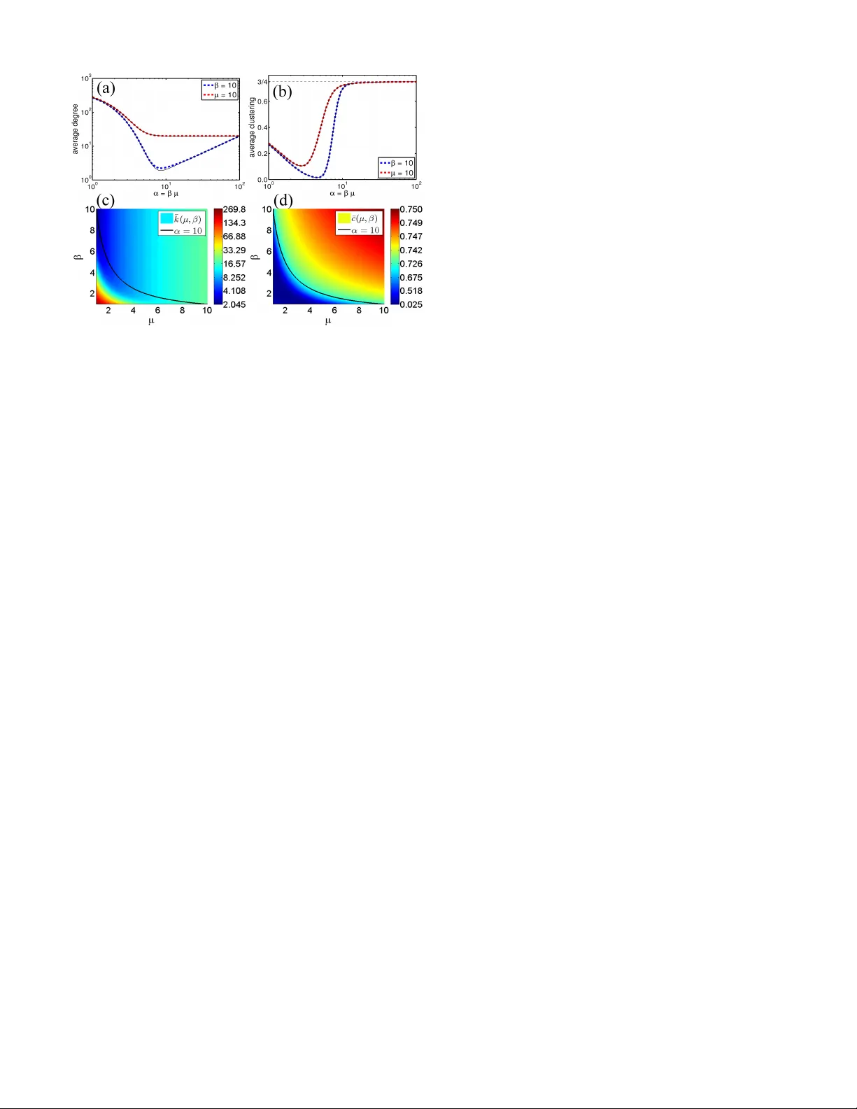
Clustering implies geometry in net w orks Dmitri Kriouk ov 1 1 Northe astern University, Dep artments of Physics, Mathematics, and Ele ctric al&Computer Engine ering, Boston, MA, USA Net work mo dels with laten t geometry ha ve been used successfully in many applications in net w ork science and other disciplines, yet it is usually imp ossible to tell if a given real netw ork is geometric, meaning if it is a typical elemen t in an ensem ble of random geometric graphs. Here w e identify structural properties of net works that guaran tee that random graphs having these properties are geometric. Sp ecifically w e show that random graphs in which exp ected degree and clustering of ev ery no de are fixed to some constants are equiv alen t to random geometric graphs on the real line, if clustering is sufficien tly strong. Large num bers of triangles, homogeneously distributed across all no des as in real netw orks, are th us a consequence of netw ork geometricity . The methods we use to pro ve this are quite general and applicable to other netw ork ensembles, geometric or not, and to certain problems in quantum gra vity . In equilibrium statistical mec hanics it is often p os sible to tell if a given system state is a typical state in a giv en ensem ble. In netw ork science, where statistical mechan- ics metho ds hav e b een used successfully in a v ariety of applications [1 – 3], the same question is often intractable. Sto c hastic net work mo dels define ensembles of random graphs with usually intractable distributions. Therefore it is usually unknown if a giv en real netw ork is a typical elemen t in the ensemble of random graphs defined by a giv en mo del, i.e., if the mo del is appropriate for the real data, so that it can yield reliable predictions. Progress has been made in addressing this problem in some classes of models, such as the configuration [4 – 10] and stochastic blo c k mo dels [11–13]. Here we are interested in latent-space netw ork mo d- els [14]. In these mo dels, nodes are assumed to p opulate some latent geometric space, while the probabilit y of con- nections betw een no des is usually a decreasing function of their distance in this space. Latent-space mo dels were first in troduced in sociology in the 70ies [15] to mo del ho- mophily in so cial net w orks—the more similar tw o p eople are, the closer they are in a laten t space, the more likely they are connected [16]. Since then, latent-space models ha ve b een used extensively in many applications, rang- ing from predicting so cial b ehavior and missing or future links [17 – 19], to designing efficien t information routing algorithms in the Internet [20] and identifying connec- tions in the brain critical for its function [21], to infer- ring comm unity structure in netw orks [14]—see [22, 23] for surveys. The simplest netw ork mo del with a latent space is the mo del with the simplest laten t space, which is the real line R 1 . No des are p oints sprinkled randomly on R 1 , and t wo nodes are connected if the distance b etw een them on R 1 is b elo w a certain threshold µ . This random graph ensem ble is known as the Gilb ert mo del of random ge- ometric graphs [24, 25]. Ev en in this simplest mo del, the ensem ble distribution is in tractable and unknown. Therefore it is imp ossible to tell if a given (real) net w ork is “geometric”—that is, if it is a typical element in the ensem ble. One can alwa ys chec k (in simulations) a sub- set of necessary conditions: if the net work is geometric, then all its structural prop erties must matc h the corre- sp onding ensemble a v erages. By “netw ork prop erty” one usually means a function of the adjacency matrix. The simplest examples of suc h functions are the num bers of edges, triangles, or subgraphs of different sizes in the net- w ork [26]. The distributions of b etw eenness or shortest- path lengths corresp ond to muc h less trivial functions of adjacency matrices. Since the num b er of such prop erty- functions is infinite, and since their inter-dependencies are in general intractable and unknown [26], it is imp os- sible to chec k if all properties match and all conditions necessary for netw ork geometricity are satisfied. Do an y sufficien t conditions exist? That is, are there any struc- tural net w ork properties such that random net w orks that ha ve these prop erties are typical elements in the ensem- ble of random geometric graphs? Here w e answer this question p ositiv ely for random ge- ometric graphs on R 1 . W e show that the set of sufficien t- condition prop erties is surprisingly simple. These prop- erties are only the exp ected num b ers of edges ¯ k and tri- angles ¯ t , or equiv alently , exp ected degree ¯ k and clus- tering ¯ c = 2 ¯ t/ ¯ k 2 of every no de. Sp ecifically , we con- sider a maxim um-entrop y ensemble of random graphs in which the exp ected degree of every no de is fixed to the same v alue ¯ k , while the exp ected num b er of trian- gles to which every no de b elongs is also fixed to some other v alue ¯ t . There is seemingly nothing geometric ab out this ensemble since it is defined in purely netw ork- structural terms—edges and triangles, in combination with the maximum-en trop y principle [27, 28]. Y et we sho w that if clustering is sufficiently strong, then this en- sem ble is equiv alen t to the ensem ble of random geometric graphs on R 1 . In general, the ensem ble is not sharp but soft [29, 30]—the probabilit y of connections is not 0 or 1 dep ending on if the distance b etw een nodes is larger or smaller than µ , but the grand canonical F ermi-Dirac probabilit y function in which energies of edges are dis- tances they span on R 1 . Strong clustering, a fundamen- 2 tally imp ortant property of real net works [31, 32], thus app ears as a consequence of their laten t geometry . The simplest model of net wor ks with strong clustering is the Strauss mo del [33] of random graphs with given exp ected num b ers of edges and triangles. The Strauss mo del is w ell studied, but many of its problematic fea- tures, including degeneracy and phase transitions with h ysteresis caused b y statistical dep endency of edges and non-con vexit y of the constraints, are not observed in real net works [27, 34, 35]. In particular, in the Strauss mo del all the triangles coalesce into a maximal clique, so that a p ortion of no des hav e a large degree and clustering close to 1, while the rest of the no des hav e a low de- gree and zero clustering [35, 36]. This clustering organi- zation differs drastically from the one in real netw orks, where triangles are homogeneously distributed across all no des, mo dulo Poisson fluctuations and structural con- strain ts [37, 38]. If we wan t to fix the exp ected num b er of edges and triangles of ev ery no de to the same v al- ues ¯ k and ¯ t , then the Strauss mo del cannot b e “fixed” to accomplish this. Therefore instead we b egin with the canonical ensemble of random graphs in which every edge { i, j } o ccurs, indep endently from other edges, with given probabilit y p ij , which in general is differen t for different edges. This ensemble is well-behav ed and void of any Strauss-lik e pathologies [2]. The exp ected degree h k i i and num ber of triangles h t i i at no de i in the ensemble are simply h k i i = P j p ij and h t i i = (1 / 2) P j,k p ij p j k p ki . An y connection probability matrix { p ij } satisfying con- strain ts h k i i = ¯ k and h t i i = ¯ t for some ¯ k , ¯ t will yield a canonical ensemble in which all no des will hav e the same exp ected degree ¯ k and num ber of triangles ¯ t . How ev er w e cannot claim that such an ensemble will b e an unbi- ased ensem ble with these constraints, b ecause a particu- lar matrix { p ij } satisfying them ma y enforce additional constrain ts on the expected v alues of some other net w ork prop erties. In other words, w e first hav e to find a wa y to sample matrices { p ij } from some maximum-en trop y distribution sub ject only to the desired constraints. This seemingly in tractable problem finds a solution us- ing the theory of graph limits known as graphons [39], with basic formalism in tro duced in netw ork mo dels with laten t v ariables [40, 41]. Graphon p ( x, y ) is a symmetric in tegrable function p : [0 , 1] 2 → [0 , 1], which is essen- tially the thermo dynamic n → ∞ limit of matrix { p ij } . F or a fixed graph size n , graphon p defines graph ensem- ble G n ( p ) b y sprinkling n no des uniformly at random on in terv al [0 , 1], and then connecting nodes i and j with probabilit y p ij = p ( x i , x j ), where x i , x j are sprinkled p o- sitions of i, j on [0 , 1]. In the n → ∞ limit, the dis- crete no de index i b ecomes contin uous x ∈ [0 , 1]. Graphs in ensemble G n ( p ) are dense, b ecause the exp ected de- gree of a no de at x ∈ [0 , 1] is h k ( x ) i = n R 1 0 p ( x, y ) dy . Here we are interested in sparse ensembles, since most real net works are sparse. Their av erage degrees are ei- ther constant or gro wing at most logarithmically with the net work size n [42]. T o mo del sparse netw orks, one can replace p ( x, y ) b y a rescaled graphon p n ( x, y ) = p ( x, y ) /n whic h dep ends on n [41, 43]. The exp ected degrees do not then dep end on n , but the num b er of triangles v anishes as 1 /n , h t ( x ) i = (1 / 2 n ) R R 1 0 p ( x, y ) p ( y , z ) p ( z , x ) dy dz , as opp osed to clustering in real netw orks, where it do es not dep end on the size of growing net works either [42]. The solution to this impasse is a linearly gro wing sup- p ort of graphon p . That is, let p : R 2 → [0 , 1] b e a graphon on the whole infinite plane R 2 . F or any finite n we simply consider its restriction to a finite square of size n × n , e.g., I 2 n , where I n = [ − n/ 2 , n/ 2], so that p n : I 2 n → [0 , 1] and p n ( x, y ) = p ( x, y ). Graphon p ( x, y ) is then the connection probability in the thermo dynamic limit. In this case, b oth the exp ected degree and n um- b er of triangles at any no de in the thermo dynamic limit can b e finite and p ositive: h k ( x ) i = R R p ( x, y ) dy and h t ( x ) i = (1 / 2) R R R 2 p ( x, y ) p ( y , z ) p ( z , x ) dy dz . F or a fi- nite graph size n , the graph ensemble G n ( p ) is defined b y sprinkling n p oints x i uniformly at random on inter- v al I n , and then connecting no des i and j with proba- bilit y p ij = p ( x i , x j ). The only difference b etw een G n ( p ) and the infinite graph ensemble G ∞ ( p ) in the thermo- dynamic limit is that in the latter case this sprinkling is a realization Π = { x i } of the unit-rate P oisson p oint pro cess on the whole infinite real line R . The main utilit y of using graphons here is that they allo w us to formalize our entrop y-maximization task as a v ariational problem which we will no w formulate. W e first observ e that for a fixed sprinkling Π, the connec- tion probability matrix { p ij } is also fixed. Since with fixed { p ij } , all edges are indep enden t Bernoulli random v ariables alb eit with different success probabilities, the en tropy of a graph ensemble S [ G n ( p | Π)] with fixed sprin- kling Π is the sum of entropies of all edges, S [ G n ( p | Π)] = (1 / 2) P i,j h ( p i,j ), where h ( p ) = − p log p − (1 − p ) log (1 − p ) is the entrop y of a Bernoulli random v ariable with the success probabilit y p . Unfixing Π no w, the distribution of entrop y S [ G n ( p | Π)] as a function of random sprinkling Π in ensemble G n ( p ) is known [44] to conv erge in the thermo dynamic limit to the delta function cen tered at the graphon entrop y s [ p ] defined b elow: S [ G n ( p | Π)] → S [ G n ( p )] → s [ p ] = 1 2 Z Z R 2 h [ p ( x, y )] dx dy , (1) where S [ G n ( p )] is the Gibbs entrop y of ensemble G n ( p ), S [ G n ( p )] = − P G ∈G n ( p ) P ( G ) log P ( G ). Bernoulli en- trop y S [ G n ( p | Π)] is thus self-av eraging, and for large n , an y graph sampled from G n ( p ) is a t ypical representa- tiv e of the ensem ble. The pro of in [44] is for dense graphons, but we show in the app endix that S [ G n ( p | Π)] is self-a veraging in our sparse settings as w ell. Therefore, our sparse ensem ble G n ( p ) is un biased if it is defined by graphon p ∗ ( x, y ) that maximizes graphon entrop y s [ p ] ab o ve, sub ject to the constraints that the exp ected num- 3 b ers of edges and triangles at ev ery no de are fixed to the same v alues ¯ k , ¯ t , h k ( x ) i = Z R p ( x, y ) dy = ¯ k , (2) h t ( x ) i = 1 2 Z Z R 2 p ( x, y ) p ( y , z ) p ( z , x ) dy dz = ¯ t. (3) T o find graphon p ∗ ( x, y ) that maximizes entrop y (1) and satisfies constrain ts (2,3), w e observe that con- strain t (2) implies that p ∗ ( x, y ) cannot be integrable since R R R 2 p ( x, y ) dx dy = ¯ k R R dx . Therefore we first hav e to solv e the problem for finite n and then consider the ther- mo dynamic limit. Using the metho d of Lagrange multi- pliers, w e define Lagrangian L = R R I 2 n dx dy { 1 2 h [ p ( x, y )] + λ k p ( x, y ) + 1 2 λ t p ( x, y ) R I n p ( y , z ) p ( z , x ) dz } with Lagrange m ultipliers λ k , λ t coupled to the degree and triangle con- strain ts. Equation δ L /δ p = 0 leads to the follo wing inte- gral equation log  1 p ( x, y ) − 1  + 2 λ k + 3 λ t Z I n p ( x, z ) p ( z , y ) dz = 0 , (4) whic h app ears intractable. Ho wev er, inspired b y the grand canonical formulation of edge-indep endent graph ensem bles [45], w e next show that for sufficiently large n, ¯ k , ¯ t , its appro ximate solution is the following F ermi-Dirac graphon p ∗ ( x, y ) = ( 1 1+ e β ( ε − µ ) = 1 1+ e 2 α ( r − 1 / 2) if 0 ≤ r ≤ 1, 1 1+ e β µ = 1 1+ e α ≡ p ∗ α if r > 1, (5) where energy ε = | x − y | ≥ 0 of edge-fermion ( x, y ) is the distance betw een no des x and y on R 1 , the chemi- cal p otential µ ≥ 0 and inv erse temp erature β ≥ 0 are functions of ¯ k and ¯ t , while α = β µ and r = ε/ 2 µ are the rescaled in verse temp erature—the logarithm of thermo- dynamic activity—and energy-distance. T o sho w this, w e first notice that if p ∗ ( x, y ) is a solu- tion, then the degree constraint (2) b ecomes ¯ k = Z I n p ∗ ( x, y ) dy = 2 µ + p ∗ α ( n − 4 µ ) ≈ 2 µ + p ∗ α n. (6) Therefore if the av erage degree ¯ k is fixed and do es not dep end on n , then p ∗ α ∼ 1 /n and α ∼ log n . If p ∗ α is small, then the last in tegral term in (4)—the exp ected n umber of common neighbors b etw een no des x and y —is negligible for r > 1 ( | x − y | > 2 µ ), and Eq. (4) sim- plifies to the equation for Erd˝ os-R ´ enyi graphs in which only the exp ected degree is fixed. Its solution is constant p ∗ ( x, y ) = 1 / (1 + e − 2 λ k ), so that λ k = − α/ 2, cf. (5). If r < 1, then the common-neighbor in tegral in (4) is no longer negligible, but we can ev aluate it exactly for p ∗ ( x, y ). The exact expression for C n ( r , α ) = 1 2 µ Z I n p ∗ ( x, z ) p ∗ ( z , y ) dz , (7) 0.0 0.2 0.4 0.6 0.8 1.0 0.0 0.2 0.4 0.6 0.8 1.0 r 1 − r C n ( r , 5) C n ( r , 10) C n ( r , 15) FIG. 1. Rescaled num ber of common neighbors C n ( r , α ) (7) v ersus 1 − r for different v alues of α = β µ ( µ = 1, n = 10 3 ). where r = | x − y | / 2 µ , is terse and non-informative, so that w e omit it for brevity . Its imp ortan t prop erty is that for large α it is closely approximated by C n ( r , α ) ≈ 1 − r , Fig. 1. In the α → ∞ limit this approximation b ecomes exact since p ∗ ( x, y ) → Θ( µ − | x − y | ) = Θ(1 / 2 − r ), where Θ() is the Heaviside step function— x and y are connected if | x − y | < µ . Approximating the common- neigh b or in tegral in (4) by 2 µ (1 − r ), and noticing that log(1 /p ∗ ( x, y ) − 1) = β ( ε − µ ) = 2 α ( r − 1 / 2), w e trans- form (4) into α ( r − 1 / 2) + λ k + 3 µλ t (1 − r ) = 0 . (8) This equation has a solution with λ k = − α/ 2 and λ t = β / 3. This solution is consisten t with the solu- tion in the r > 1 regime. First, the v alue of λ k is the same in b oth regimes r < 1 and r > 1. Second, one can c heck that the exp ected n umber of common neighbors R I n p ∗ ( x, z ) p ∗ ( z , y ) dz deca ys exp onen tially with α for any r > 1. Therefore the common neighbor term in (4) is in- deed negligible in the r > 1 regime, even though the prefactor 3 λ t = α/µ is large for fixed µ and large α . Figure 2 illustrates that if α is large, then the expected a verage degree ¯ k (6) and clustering ¯ c = 2 ¯ t ¯ k 2 = 1 ¯ k 2 Z Z I 2 n p ∗ ( x, y ) p ∗ ( y , z ) p ∗ ( z , x ) dy dz (9) in ensemb le G n ( p ∗ ) are functions of only µ and α , resp ec- tiv ely . Giv en v alues of the t w o constrain ts ¯ k and ¯ t (or ¯ c ) define the t wo ensem ble parameters µ and β (or α ) as the solution of Eqs. (6,9). W e note that for large α ( α > 10 in Fig. 2), clustering is close to its maximum ¯ c max = 3 / 4 ( ¯ t max = 3 µ 2 / 2), which can b e computed analytically . Since our appro ximations are v alid only for large α , they apply only to graphs with strong clustering. In the sparse thermo dynamic limit n → ∞ with a finite av erage degree ¯ k , the chemical p otential µ m ust b e finite and α must di- v erge (temp erature T = 1 /β m ust go to zero) b ecause of (6), so that only graphs with the strongest clustering are the exact solution to our entrop y-maximization prob- lem. F or finite n how ev er, higher-temp erature graphs with weak er clustering are an approximate solution. W e emphasize that the fact that graphon (5), in which the dep endency on x and y is only via distance ε = | x − y | , 4 FIG. 2. Average degree (a,c) and clustering (b,d) in soft random geometric graphs with connection probabilit y (5) as functions of µ and β . The dashed curves in (a,b) show the sim ulation results av eraged ov er 100 random graphs of size n = 10 3 on the interv al [ − 500 , 500] with p erio dic b oundary conditions. The solid curves in (a,b) and color in (c,d) are the (corresp onding) analytic results using (6) in (a,c) , and n umeric ev aluation of (9) in (b,d) with n = 10 3 . The color axes in (c,d) are in the logarithmic scale, with color tic ks ev enly spaced in log ¯ k in (c) and log (3 / 4 − ¯ c ) in (d) . is an approximate entrop y maximizer, means that the en- sem ble of random graphs in which the exp ected degree and clustering of every no de are fixed to given constan ts, is approximately equiv alen t to the ensemble of soft ran- dom geometric graphs with the sp ecific form of the con- nection probability , i.e., the grand canonical F ermi-Dirac distribution function that maximizes ensemble en tropy constrained b y fixed a verage energy and n umber of par- ticles. In our ensemble, F ermi particles are graph edges (0 or 1 edge b etw een a pair of no des), and their energy is the distance they span on R 1 . The av erage num b er of particles ¯ m = ¯ k n/ 2 is fixed by c hemical p otential µ . Fixing av erage energy ¯ ε and fixing the av erage num ber of triangles ¯ t are equiv alen t b ecause the smaller the ¯ ε , the more likely the lo wer-energy/smaller-distance states, the larger the ¯ t thanks to the triangle inequality in R 1 . This equiv alence explains why the F ermi-Dirac distribu- tion (5) app ears as an approximate solution to our en- trop y maximization problem constrained b y fixed ¯ k and ¯ t . In the zero-temp erature limit β → ∞ , graphon (5) b ecomes the step function p ∗ ( x, y ) = Θ( µ − ε ), mean- ing that these soft random geometric graphs b ecome the traditional sharp random geometric graphs in whic h any pair of no des is connected if their distance-energy is at most µ . All the approximations b ecome exact in this limit. The degree distribution in (soft) random geometric graphs is the P oisson distribution [25], while in man y real net works it is a pow er la w. T riangles in real net works are still homogeneously distributed across all no des, alb eit sub ject to non-trivial structural constraints imp osed b y the pow er-la w degree distribution [26, 37, 38]. As shown in [46, 47], random geometric graphs on R 1 can b e gen- eralized to satisfy an additional constraint enforcing a p o wer-la w degree distribution. This generalization still uses the grand canonical F ermi-Dirac connection proba- bilit y , alb eit in hyperb olic geometry , and repro duces the clustering organization in real netw orks. These observ a- tions lead to the conjecture that real scale-free net works are typical elements in ensembles of soft random geo- metric graphs with non-trivial degree distribution con- strain ts. If so, then non-trivial communit y structure, an- other common feature of real netw orks, is a reflection of non-uniform no de density in laten t geometry [14, 48]. As a final remark w e note that the graphon-based metho dology w e developed here is quite general and can b e applied to other net work models with laten t v ariables, geometric or not, to tell if a given mo del is adequate for a giv en net work. W e also note that a v ery similar class of problems underlies approaches to quantum gravit y with emerging geometry [23, 49] where one exp ects contin u- ous spacetime to emerge in the classical limit from fun- damen tally discrete physics at the Planc k scale. Perhaps the most directly related example is the Hauptv ermutung problem in causal sets [50, 51]. Giv en a Lorentzian space- time, causal sets are random geometric graphs in it with edges connecting timelik e-separated pairs of even ts sprin- kled randomly onto the spacetime at the Planc k density . If no contin uous spacetime is given to b egin with, then what discrete physics can lead to an ensemble of random graphs equiv alen t to the ensem ble of causal sets sprin- kled onto the spacetime that we observ e? T o answer this question, one has to solve the same ensemble equiv alence problem as we solv ed here, except not for R 1 , but for the spacetime of our Universe. App endix Here we sho w that entrop y of the considered sparse graph ensemble is self-av eraging. F or completeness, we first sho w that a verage entrop y density conv erges to graphon entrop y densit y in the thermo dynamic limit, and then show that the relative v ariance (co efficient of v aria- tion) of the en trop y distribution go es to zero in this limit. W e b egin with notations and definitions. Notations and definitions. Let I n = [ − n/ 2 , n/ 2] b e the interv al of length n , and Π = { x i } , i = 1 , 2 , . . . , n b e n real num bers sampled uniformly at random from I n . F or large n , binomial sampling Π approximates the P oisson p oint pro cess of unit rate on I n . Since ev ery x i is uniformly distributed on I n , and since all x i s are inde- p enden t, the probabilit y density function of sprinklings 5 Π is P (Π) = 1 n n . (10) W e impose the p erio dic b oundary conditions on I n mak- ing it a circle, so that the distance b etw een p oint i and j is x ij = n 2 −    n 2 − | x i − x j |    . (11) Distances { x ij } are uniformly distributed on [0 , n/ 2]. Giv en Π, ensemble G n ( p | Π) is the ensem ble of graphs whose edges, or elements of adjacency matrix { a ij } , are indep enden t Bernoulli random v ariables: abusing nota- tion for p , a ij = 1 with probability p ij = p ( x i , x j ) = p ( x ij ), and a ij = 0 with probabilit y 1 − p ij . There are no self-edges, so that p ii = 0. The entrop y of random v ariable a ij is h ( p ij ), where h ( x ) = − x log x − (1 − x ) log (1 − x ) (12) is the entrop y of the Bernoulli random v ariable with suc- cess probability x . Since all a ij s are indep enden t in en- sem ble G n ( p | Π), its entrop y is S n ≡ S n (Π) ≡ S [ G n ( p | Π)] = 1 2 n X i,j =1 h ( p ij ) , (13) whic h is fixed for a giv en sprinkling Π. Ensem ble G n ( p ) is the ensem ble of graphs sampled by first sampling random sprinkling Π, and then sampling a random graph from G n ( p | Π). W e consider entrop y S n as a random v ariable defined b y Π. This random v ariable is self-av eraging if its relativ e v ariance v anishes in the thermo dynamic limit, c v = p h S n − h S n ii 2 h S n i − − − − → n →∞ 0 , (14) where h·i stands for a veraging across random sprin- klings Π. W e first sho w that av erage en tropy density— that is, a verage entrop y p er no de h S n i /n —con verges to graphon entrop y densit y σ , h S n i n − − − − → n →∞ σ 2 , (15) σ = lim n →∞ σ n = Z R h [ p ( x ij )] dx ij , (16) σ n = s n n = Z I n h [ p ( x ij )] dx ij , (17) s n = Z Z I 2 n h [ p ( x i , x j )] dx i dx j , (18) and then prov e (14). F or notational conv enience in the equations ab ov e, w e ha v e extended the supp ort of p ( x ij ) from R + to R by p ( − x ij ) = p ( x ij ). Av erage ensemble en trop y density con v erges to graphon entrop y density . Using the definitions and observ ations ab o ve, we get h S n i n = 1 n Z I n n S n (Π) P (Π) Y k dx k (19) h S n i n = 1 2 n Z I n n X i,j h [ p ( x i , x j )] P (Π) Y k dx k (20) = 1 2 n n +1 Z I n n X i,j h [ p ( x i , x j )] Y k dx k . (21) The in tegration o ver n − 2 v ariables x k with indices k not equal to either i or j yields the factor of n n − 2 : h S n i n = 1 2 n 3 X i,j Z Z I 2 n h [ p ( x i , x j )] dx i dx j , (22) where we ha ve also swapped the summation and integra- tion. Changing v ariables from x i and x j to x ij and x j , and integrating ov er x j yields another factor of n : h S n i n = 1 2 n 2 X i,j Z I n h [ p ( x ij )] dx ij . (23) Since x ij are uniformly distributed on [0 , n/ 2], all terms in the sum con tribute equally , bringing another factor of n ( n − 1) ≈ n 2 , the total num ber of terms in the sum: h S n i n = 1 2 Z I n h [ p ( x ij )] dx ij = σ n 2 . (24) W e th us hav e that h S n i n − − − − → n →∞ 1 2 lim n →∞ σ n = σ 2 . (25) Ensem ble en trop y is self-a v eraging. T o compute c v = p h S 2 n i − h S n i 2 h S n i (26) w e must calculate h S 2 n i = *   1 2 X i,j h [ p ( x i , x j )]   2 + (27) = I 1 + I 2 , where (28) I 1 = 1 4 Z I n n X i,j h 2 [ p ( x i , x j )] P (Π) Y m dx m , (29) I 2 = 1 4 Z I n n X i,j ; k ,l h [ p ( x i , x j )] h [ p ( x k , x l )] P (Π) Y m dx m . (30) The first in tegral I 1 is different from (20) only in that instead of h/ 2 we now ha ve ( h/ 2) 2 . Therefore w e imme- diately conclude that I 1 = n 4 γ n , where (31) γ n = Z I n h 2 [ p ( x )] dx. (32) 6 If σ n = R I n h [ p ( x )] dx conv erges to finite σ in the n → ∞ limit, as it do es for the F ermi-Dirac p ∗ , then so do es γ n , γ n − − − − → n →∞ γ < ∞ , because h ( p ) ∈ [0 , 1]. T o calculate the second in tegral I 2 , we use P (Π) = 1 /n n and integrate ov er n − 4 v ariables x m with indices m not equal to any i, j, k , l , bringing the factor of n n − 4 : I 2 = 1 4 n 4 X i,j ; k ,l Z Z Z Z I 4 n h [ p ( x i , x j )] h [ p ( x k , x l )] dx i dx j dx k dx l . (33) Changing v ariables from x i , x j , x k , and x l , to x ij , x j , x kl , and x l , and integrating o v er x j and x l , thus bringing another factor of n 2 , we get: I 2 = 1 4 n 2 X i,j ; k ,l Z Z I 2 n h [ p ( x ij )] h [ p ( x kl )] dx ij dx kl . (34) Since x ij and x kl are indep endent and uniformly dis- tributed on [0 , n/ 2], every term in the double sum con- tributes equally , while the total num ber of terms is [ n ( n − 1)] 2 ≈ n 4 , yielding I 2 = n 2 4 Z Z I 2 n h [ p ( x ij )] h [ p ( x kl )] dx ij dx kl (35) =  n 2 Z I n h [ p ( x )] dx  2 (36) =  n 2 σ n  2 = h S n i 2 . (37) Collecting the calculations of h S n i and h S 2 n i , we finally obtain c v = p I 1 + I 2 − h S n i 2 h S n i = p ( n/ 4) γ n ( n/ 2) σ n = 1 √ n √ γ n σ n . (38) If σ n − − − − → n →∞ σ < ∞ , then γ n − − − − → n →∞ γ < ∞ , and c v = 1 √ n √ γ n σ n − − − − → n →∞ 0 . (39) W e thank G. Lippner, P . T opalov, M. Piskuno v, M. Kitsak, M. Bogu ˜ n´ a, S. Horv´ at, Z. T oro czk ai, and Y. Baryshniko v for useful discussions and suggestions. This work was supported b y NSF CNS-1442999. [1] R. Alb ert and A.-L. Barab´ asi, Rev Mod Phys 74 , 47 (2002). [2] J. Park and M. E. J. Newman, Phys Rev E 70 , 66117 (2004). [3] J. Gao, B. Barzel, and A.-L. Barab´ asi, Nature 530 , 307 (2016). [4] G. Bianconi, Eur Lett 81 , 28005 (2008). [5] G. Bianconi, P . Pin, and M. Marsili, Pro c Natl Acad Sci USA 106 , 11433 (2009). [6] K. Anand and G. Bianconi, Phys Rev E 80 , 045102(R) (2009). [7] K. Anand, D. Kriouko v, and G. Bianconi, Phys Rev E 89 , 062807 (2014). [8] D. Garlaschelli and M. Loffredo, Phys Rev E 78 , 015101 (2008). [9] D. Garlaschelli and M. Loffredo, Phys Rev Lett 102 , 38701 (2009). [10] T. Squartini, R. Mastrandrea, and D. Garlaschelli, New J Phys 17 , 023052 (2015). [11] T. P . P eixoto, Phys Rev E 85 , 056122 (2012). [12] T. P . P eixoto, Phys Rev Lett 110 , 148701 (2013). [13] T. P . P eixoto, Phys Rev X 4 , 011047 (2014). [14] M. E. J. Newman and T. P . Peixoto, Ph ys Rev Lett 115 , 088701 (2015). [15] D. D. McF arland and D. J. Brown, in Bonds of Plur alism: The F orm and Substance of Urb an So cial Networks (John Wiley , New Y ork, 1973) pp. 213–252. [16] M. McPherson, L. Smith-Lovin, and J. M. Co ok, Ann u Rev So ciol 27 , 415 (2001). [17] P . D. Hoff, A. E. Raftery , and M. S. Handco ck, J Am Stat Asso c 97 , 1090 (2002). [18] P . Sark ar, D. Chakrabarti, and A. W. Mo ore, in IJCAI (2011) pp. 2722–2727. [19] G. Tita, P . J. Bran tingham, A. Galst y an, and Y.-S. Cho, Discret Contin Dyn Syst - Ser B 19 , 1335 (2014). [20] M. Bogu ˜ n´ a, F. Papadopoulos, and D. Kriouko v, Nat Comm un 1 , 62 (2010). [21] A. Guly´ as, J. J. B ´ ır´ o, A. K˝ or¨ osi, G. R ´ etv´ ari, and D. Kri- ouk ov, Nat Commun 6 , 7651 (2015). [22] M. Barth ´ elemy , Ph ys Rep 499 , 1 (2011). [23] G. Bianconi, EPL 111 , 56001 (2015). [24] E. N. Gilb ert, J Soc Ind Appl Math 9 , 533 (1961). [25] M. P enrose, R andom Ge ometric Gr aphs (Oxford Univer- sit y Press, Oxford, 2003). [26] C. Orsini, M. M. Dankulo v, P . Colomer-de Sim´ on, A. Ja- mak ovic, P . Mahadev an, A. V ahdat, K. E. Bassler, Z. T oro czk ai, M. Bogu ˜ n´ a, G. Caldarelli, S. F ortunato, and D. Kriouk ov, Nat Commun 6 , 8627 (2015). [27] S. Horv´ at, ´ E. Czabark a, and Z. T oro czk ai, Phys Rev Lett 114 , 158701 (2015). [28] T. Squartini, J. de Mol, F. den Hollander, and D. Gar- lasc helli, Ph ys Rev Lett 115 , 268701 (2015). [29] C. P . Dettmann and O. Georgiou, Ph ys Rev E 93 , 032313 (2016). [30] M. P enrose, Ann Appl Probab 26 , 986 (2016). [31] F. Radicchi, C. Castellano, F. Cecconi, V. Loreto, and D. Parisi, Pro c Natl Acad Sci 101 , 2658 (2004). [32] F. Radicchi and C. Castellano, Phys Rev E 93 , 030302 (2016). [33] D. Strauss, SIAM Rev 28 , 513 (1986). [34] D. F oster, J. F oster, M. Paczuski, and P . Grassb erger, Ph ys Rev E 81 , 046115 (2010). [35] J. Park and M. E. J. Newman, Phys Rev E 72 , 026136 (2005). [36] C. Radin, K. Ren, and L. Sadun, J Phys A Math Theor 47 , 175001 (2014). [37] P . Colomer-de Sim´ on, M. ´ A. Serrano, M. G. Beir´ o, J. I. Alv arez-Hamelin, and M. Bogu˜ n´ a, Sci Rep 3 , 2517 (2013). [38] V. Zlati´ c, D. Garlaschelli, and G. Caldarelli, EPL 97 , 7 28005 (2012). [39] L. Lov´ asz, L ar ge Networks and Gr aph Limits (American Mathematical So ciety , Pro vidence, RI, 2012). [40] G. Caldarelli, A. Cap o cci, P . D. L. Rios, and M. A. Mu ˜ noz, Phys Rev Lett 89 , 258702 (2002). [41] M. Bogu ˜ n´ a and R. Pastor-Satorras, Phys Rev E 68 , 36112 (2003). [42] S. Boccaletti, V. Latora, Y. Moreno, M. Chav ez, and D.-U. Hwanga, Phys Rep 424 , 175 (2006). [43] C. Borgs, J. T. Chay es, H. Cohn, and Y. Zhao, [44] S. Janson, NYJM Monogr 4 (2013), [45] D. Garlasc helli, S. E. Ahnert, T. M. A. Fink, and G. Cal- darelli, Entrop y 15 , 3148 (2013). [46] M. ´ A. Serrano, D. Kriouko v, and M. Bogu ˜ n´ a, Phys Rev Lett 100 , 78701 (2008). [47] D. Kriouko v, F. Papadopoulos, M. Kitsak, A. V ahdat, and M. Bogu˜ n´ a, Ph ys Rev E 82 , 36106 (2010). [48] K. Zuev, M. Bogu˜ n´ a, G. Bianconi, and D. Kriouk ov, Sci Rep 5 , 9421 (2015). [49] Z. W u, G. Menichetti, C. Rahmede, and G. Bianconi, Sci Rep 5 , 10073 (2015). [50] R. Sorkin, in L e ctur es on Quantum Gr avity , edited by A. Gomberoff and D. Marol (Springer, New Y ork, 2005) pp. 305–328. [51] L. Bombelli, J. Lee, D. Meyer, and R. Sorkin, Ph ys Rev Lett 59 , 521 (1987).