Convex Optimization for Linear Query Processing under Approximate Differential Privacy

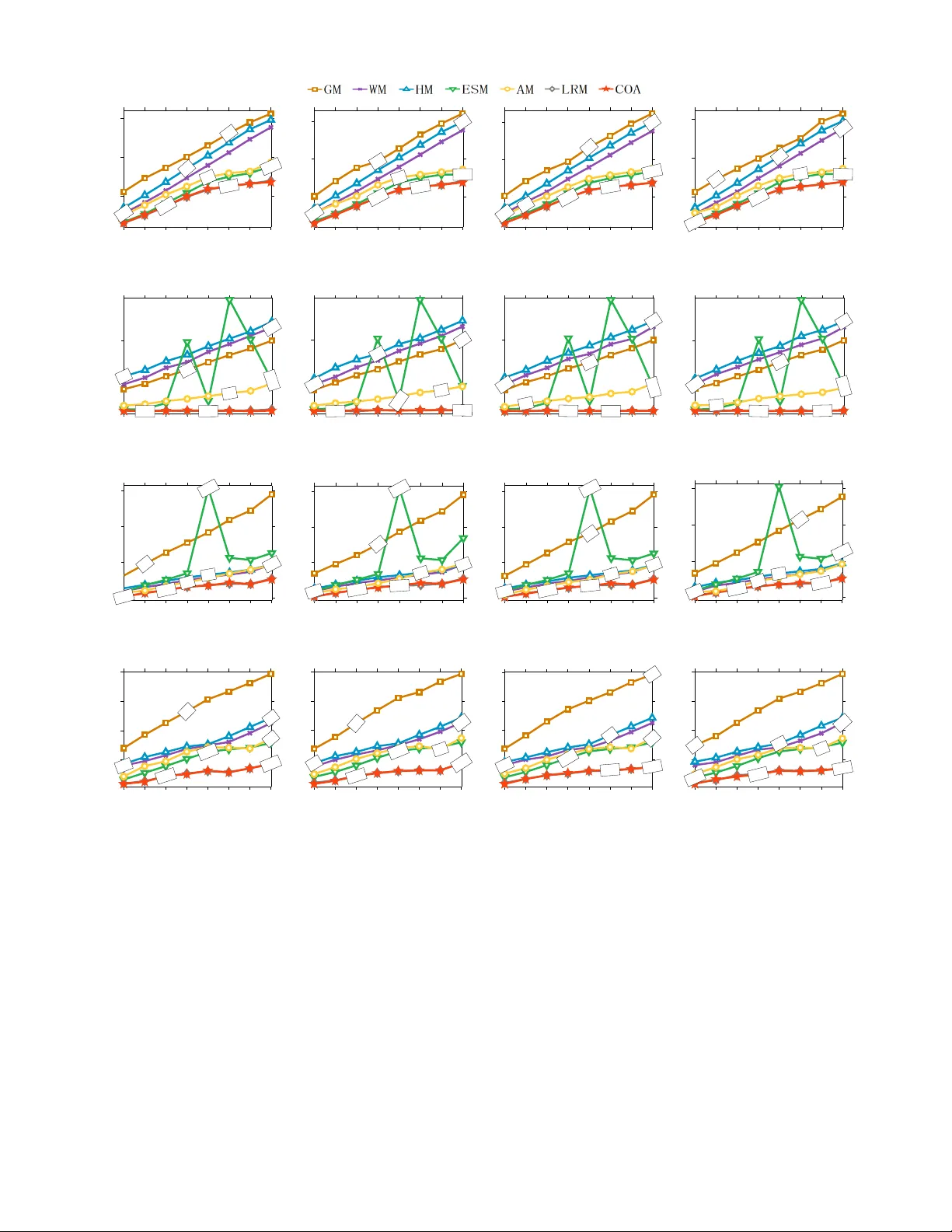
Con ve x Optimization fo r Linear Query Pro cessing under Appr o ximate Differential Priv acy Ganzhao Y uan 1 Y in Y an g 2 Zhenjie Zhang 3 Zhif eng Hao 4 1 School of Mathematics, South China Univ ersity of T echno logy , yuangan zhao@gmail .com 2 College of Science and Engine er ing, Hamad Bin Khalif a University , yyang @qf.org.qa 3 Adv anced Digital Sciences Center , Illinois at Singapor e Pte. Ltd., zhenjie @adsc.com.sg 4 School of Mathematics and Big Data, F oshan University , mazfhao@scut.edu.cn ABSTRA CT Differential priv acy enables organ izations to collect accurate aggre- gates ov er sensiti ve data with strong, rigorous guarantees on indi- viduals’ pri vacy . Previo us work has found t hat under differe ntial priv acy , comp uting multiple correlated ag gregates as a batch, using an appropriate st rate gy , may yield higher accuracy than comput- ing each of them ind ependently . Howe ver , ﬁ nding the b est strategy that maximizes result accurac y is non-tri vial, as it i n volv es solv- ing a comple x con st rained optimization prog ram that appears to be non-linear and non-con vex. Hence, in the past much effort has been de voted in so lving this n on-con vex optimization prog ram. E xisting approaches include various sophisticated heuristics and exp ensive numerical solution s. None o f them, ho we ver , guarantees to ﬁ nd the optimal solution of this optimization problem. This paper points out that under ( ǫ , δ )-differential pri vac y , the optimal solution of the abov e constrained op timization pro blem in search of a suitable strategy can be found, rather surprisingly , by solving a simple and elegant con vex optimization program. Then, we propose an efﬁcient algorithm based on Newton’ s method, which we prove to always con verge to the optimal solution with linear global con vergen ce rate and quadratic local con ver gence rate. Em- pirical ev aluations demonstrate the accuracy and ef ﬁciency of the proposed solution. 1. INTR ODUCTIO N Differential pri vac y [5, 3] is a strong and rigorous priv acy pro- tection mode l that is kno wn for its generality , robu stness and ef fec- tiv eness. It i s used, for ex ample, in the ubiquitous Goo gle Chrome bro wser [7]. The main idea is to publish randomized aggregate in- formation ov er sensitiv e data, with the guarantee that the adversary cannot infer with high conﬁdence the presence or absence of any in- di vidual in the dataset from the released aggregates. An important goal in the design of dif ferentially pri vate methods is to maximize the accurac y of the pu blished noisy aggre gates with respect to the ir exact v alues. Besides optimizing for speciﬁc types of aggregates, an i mpor - tant generic methodology for i mprov i ng the ov erall accuracy of the released aggre gates under differen tial priv acy is batch pr ocessing , Permission to make digital or hard copies of all or pa rt of this work for personal or classroom us e is granted without fee provided that copies a re not made or distribut ed for proﬁ t or commercial advantage and that copies bear this notice and the full cita- tion on the ﬁrst page. Copyrights for components of this w ork owned by other s than ACM mu st be honor ed. Abstracting with credit is permitt ed. T o copy otherwise, or r e - publish, to pos t on se rvers or to redistribute to lists, requires prior speciﬁc permission and /or a fee. Request permissions from permissions@acm.org. c  2018 ACM. ISBN 978-1-4503- 2138-9. DOI: 10.1145/1235 ﬁrst proposed in [13]. Speciﬁcally , batch processing exploits the correlations between multiple queries, so that answering t he batch as a wh ole can lead to higher o verall accurac y than answering each query indiv idually . For examp l e, if one aggre gate query Q1 (e.g., the total population of New Y ork State and New Jerse y) can be ex- pressed as the sum of two other queries (the population of Ne w Y ork and New Jersey , respectiv ely), i.e., Q1 = Q2 + Q3, t hen we can simply answer Q1 by adding up the noisy answers of Q2 and Q3. Intuitiv ely , answering two queries instead of three r educes the amount of ran dom perturbations required to sa tisfy dif ferential pri- v acy , leading to higher ov erall accurac y for the batch as a whole [13, 30]. In this paper , we f ocus on answering linear aggreg ate queries under differential priv acy . Giv en a batch of linear ag gregate queries (called the workload ), we aim to improv e their ov erall ac- curacy by answering a different set of queries (called the strate gy ) under dif ferential priv acy , and combining their results to o btain the answers to the original workloa d aggregates. As shown in [13, 14, 30, 31, 11], dif f erent strategy queries lead to different overall accurac y for the original workload. Hence, an important problem in b atch processing un der diffe rential priv acy is to ﬁnd a suitable strategy t hat leads to the highest accurac y . Such a strategy can be rather complex, rendering manual construction and brute-force search infeasible [ 30, 31]. On the other hand, the problem of strategy searching can be formu lated into a constrained optimization prog ram, and it sufﬁces to ﬁnd t he optimal solution of this program. Ho we ver , as we show later in Section 2, the program appears to be non-linea r and non-con ve x; hence, solving it is rath er challenging. As we revie w in Section 2.2, existing approaches re- sort to either heu r istics or com plex, expe nsi ve and u nstable numer - ical metho ds. T o our kno wledge, no e xisting solutions guarantee to ﬁnd the optimal solution. This paper points out that under the ( ǫ , δ )-differential priv acy deﬁnition (also called approximate differential pri vacy , explained in Section 2), the constrained optimization program for ﬁnding the best s trategy queries can be re-formulated into a simple and ele gant con ve x optimization program. Note that although the formulation itself is simple, it s deri v ati on is rather complicated and non-trivial. Based on t his new formulation, we propose the ﬁrst polynomial solution COA that guara ntees to ﬁnd t he optimal solution to t he original constrained optimization problem in search of a suitable strategy for processing a batch o f arbitrary linear aggregate qu eries under approximate dif ferential priv acy . CO A is based on Newton ’ s method an d it utilizes v ari ous no n-trivial pro perties of the p roblem. W e sho w that COA achie ves globally linear and locally quadratic con verg ence rate. Extensiv e experiments conﬁrm the effecti veness and efﬁcienc y of the proposed method. The rest of the paper is organized as follo ws. Section 2 provides necessary backgrou nd on differen t ial priv acy and overvie ws related work. Section 3 presents our con vex programming f ormulation for batch linear aggregate processing under approximate differential priv acy . Section 4 describes the proposed solution COA. Section 5 contains a thorough set o f exp eri ments. Section 6 c oncludes t he pa- per with directions for future work. In this paper , boldfaced lower- case letters denote v ectors and uppercase letters deno te real-valued matrices. W e summarize the frequent notations i n T able 1 . T able 1: Summary of frequent notations Symbol Meaning W W ∈ R m × n , W orkload matrix m Number of queries (i.e., ro ws) i n W n Unit counts (i.e., columns) in W V V ∈ R n × n , Cov ariance matrix of W X X ∈ R n × n , Solution matrix A A ∈ R p × n , Strategy matrix A † A † ∈ R n × p , pseudo-in verse of matrix A v ec ( X ) v ec ( X ) ∈ R n 2 × 1 , V ectorized listing of X mat ( x ) mat ( x ) ∈ R n × n , Con vert x ∈ R n 2 × 1 into a matrix F ( X ) F ( X ) ∈ R , Objective v alue of X G ( X ) G ( X ) ∈ R n × n , Gradient matrix of X H ( X ) H ( X ) ∈ R n 2 × n 2 , Hessian matrix of X H X ( D ) H X ( D ) ∈ R n × n , Equi valent to mat ( H ( X ) v ec ( D )) 1 / 0 All-one column vector/All-zero column v ector I Identity matrix X  0 Matrix X is positi ve semideﬁnite X ≻ 0 Matrix X is positi ve deﬁnite λ ( X ) Eigen value of X (increasing orde r) diag ( x ) Diagonal matrix with x as the main diagonal entries diag ( X ) Column vector formed from the main diag onal of X k X k Operator norm: the largest eigen va lue of X χ ( X ) Smallest eigen value of X tr ( X ) Sum of the elements on the main diagonal X h X , Y i Euclidean inner produc t, i. e., h X , Y i = P ij X ij Y ij X ⊗ Y Kroneck er product of X and Y X ⊙ Y Hadamard (a.k.a. entry-wise) product of X and Y k X k ∗ Nuclear norm: sum of the singular values of matrix X k X k F Frobenius norm: ( P ij X 2 ij ) 1 / 2 k X k N Generalized vector norm: k X k N = ( v e c ( X ) T N v ec ( X )) 1 / 2 C 1 , C 2 lo wer bound and upper bound of λ ( X ) C 3 , C 4 lo wer bound and upper bound of λ ( H ( X )) C 5 , C 6 lo wer bound and upper bound of λ ( G ( X )) 2. B A CKGROUND 2.1 Pr elimi naries A common deﬁnition of dif ferential pri vacy is ( ǫ , δ )-differen t ial priv acy [5], as follows: D E FI N IT I O N 1 . T wo databases D and D ′ ar e neighboring iff the y differ by at most one tuple. A rando mized algorithm M satis- ﬁes ( ǫ, δ )-differ ential privacy iff for any two ne ighboring da tabases D and D ′ and any measurab le output S in t he rang e of M , we have Pr[ M ( D ) ∈ S ] ≤ e ǫ · Pr[ M ( D ′ ) ∈ S ] + δ. When δ = 0 , the abov e deﬁnition reduces to another popular deﬁnition: ǫ -differen tial pri v acy (also called “e xact differen tial pri- v acy”). This w ork focu ses o n the case wh ere δ > 0 , which is some- times called approximate differen tial priv acy . Usually , δ is set t o a v alue small er t han 1 | D | , where | D | is the number of records in the dataset D . Both exact and approximate deﬁnitions of differential priv acy pro vide strong and rigorous priv acy protection to the users. Giv en the output of a dif ferentiall y priv ate mechanism, the adver - sary cannot i nfer with high conﬁdence (controlled by parameters ǫ and δ ) whether the original database is D or any of its neighbo rs D ′ , which differ fro m D by one record, meaning that ea ch user can plausibly deny the presence of her tuple. An approximately differ- entially priv ate mechanism can be understood as satisfying exact differe ntial priv acy with a certain probability controlled by param- eter δ . Hence, it is a more relaxe d deﬁnition which i s parti cularly useful when the exact deﬁnition is ov erly st rict for an application, leading to poor result utility . One basic mech anism for e nforcing approximate d i f ferential pri- v acy is the Gaussian mechanism [4], which injects Gaussian noise to the query results calibrated to the ℓ 2 sensitiv i ty of the queries. Note t hat the Gaussian mechanism cannot be applied to exact dif- ferential priv acy . S ince the prop osed method is based on the Gaus- sian mechanism, it i s limited to query processing under approxi- mate differential pri v acy as well. S peciﬁcally , for any two neigh- bor databases D and D ′ , the ℓ 2 sensitiv i ty Θ( Q ) of a query s et Q is deﬁned as Θ( Q ) = max D ,D ′ k Q ( D ) , Q ( D ′ ) k 2 . Giv en a databa se D and a query set Q , the Gaussian mechanism outputs a random result that follows t he Gaussian distribution wi th mean Q ( D ) and magnitude σ = Θ( Q ) /h ( ǫ, δ ) , where h ( ǫ, δ ) = ǫ/ p 2 ln(2 /δ ) . This paper focuses on answering a batch of m linear aggregate queries, Q = { q 1 , q 2 , . . . , q m } , each of which is a linea r combina- tion of the unit aggregates of the input database D . For simplicity , in the following we assume that each unit aggregate is a simple count, which has an ℓ 2 sensitiv i ty of 1. Other types of aggre gates can be handled by adjusting t he sensitivity accordingly . The query set Q can be represented by a workload matrix W ∈ R m × n with m ro ws and n columns. Each entry W ij in W is the weight in query q i on the j - th unit count x j . S ince we do not use any other infor- mation of the i nput database D besides the unit counts, in the fol- lo wing we abuse the no t ation by using D to represent the ve ct or of unit coun ts. Therefore, we deﬁne D , x ∈ R n , Q , W ∈ R m × n (“ , ” means deﬁne). The query batch Q can be answered directly by: Q ( D ) , Wx = X j W 1 j x j , . . . , X j W mj x j ! T ∈ R m × 1 Giv en a work load matrix W , the worse-case expected squared error of a mechanism M is deﬁned as [13, 15, 20]: er r ( M ; W ) , max x ∈ R n E [ kM ( x ) − Wx k 2 2 ] where the e xpectation is taken ove r the randomness of M . W i thout information of the underlying dataset, the lo west error achiev able by any differentially priv ate mechanism for the query matrix W and database is: opt ( W ) = min M er r ( M ; W ) (1) where the i nﬁmum is taken ove r all differe ntially priv ate mecha- nisms. If a mechan ism M minimizes the objectiv e value in Eq (1), it is the optimal linear counting query processing mechanism, in the sense that without any p r ior information of the sensiti ve data, it achie ves the lowest exp ected error . 2.2 Existing Solutions Matrix Mechani sm. The ﬁrst solution f or answering batch li n- ear aggre gate queries und er dif ferential pri v acy is the matrix mec h- anism [13]. The main i dea is that instead of answering the workload queries W directly , the mechanism ﬁrst answers a dif ferent set of r queries under differential priv acy , and t hen combine their results to answer W . Let matrix A represent the strategy queries, where each ro w represent a query and each column represe nt a unit co unt. Then, according to the Gaussian mechanism, A can be answered using Ax + ˜ b under ( ǫ, δ ) -dif ferentially priv acy , where ˜ b denotes an m dimensional Gaussian variable with scale || A || 2 , ∞ p 2 ln(2 /δ ) /ǫ , and k A k p, ∞ is the maximum ℓ p norm among all column vectors of A . Accordingly , t he matrix mechanism answers W by: M ( x ) = W ( x + A † ˜ b ) (2) where A † is the Moore-Penrose pseudo-in verse of A . Based on Eq ( 2), Li et al. [13] formalize the strategy searching problem for batch linear counting query processing in E q(1) into the follo wing nonlinear optimization problem: min A \{ 0 } J ( A ) , k A k 2 p, ∞ tr ( W A † A † T W T ) . (3) In the abov e optimization program, p can be either 1 or 2, and the method in [13] applies to both exact and approximate differen- tial priv acy . This optimization program, howe ver is rather difﬁcult to solve. The pseudo in verse of A † of A inv olved in P rogram (3) is not a continuous function, as i t jumps around when A is ill- conditioned. Therefore, A † does not have a deri v ative, and we cannot solve the problem with simple gradient descent. As pointed out in [31], the solutions in [13] are either prohibitively expensi ve (which needs t o iterative ly solve a pair of related semideﬁnite pro- grams that incurs O ( m 3 n 3 ) computational costs), or ineffecti ve (which rarely obtains strategies that outp erform naiv e methods). Low-Rank Mechanism. Y uan et al. [31] propose the Low-Rank Mechanism (LRM), which formulates the batch query problem as the follo wing low-rank matrix f actorization problem: min B , L tr ( B T B ) s.t. W = BL , k L k p, ∞ ≤ 1 (4) where B ∈ R m × r , L ∈ R r × n . It can be sho wn that P rogram (4) and Program (3 ) are equiv alent to each other; hence, LRM can be vie wed as a way to solve t he Matrix Mechanism optimization pro- gram (to our kno wl edge, LRM is also the ﬁrst practical so l ution for this program). The LRM formulation avoids the pseudo-in verse of the st rategy matrix A ; howe ver , it is sti ll a non-linear , non-con ve x constrained optimization program. Hence, it is also difﬁcult to solve. The solution i n LRM is a sophisticated numeric method based ﬁrst-order augmented Lagrangian multipliers (ALM). T his solution, howe ver , cannot guarantee to ﬁnd t he globally optimal strategy matrix A , due to t he non-con vex nature of the problem formulation. Further , the LRM solution may not con verge at all. Speciﬁ- cally , i t iterati vely updates B using the formula: B ⇐ ( β WL T + π L T )( β LL T + I ) − 1 , where β is the penalty parameter . When L is low-rank , according to the rank inequality for matri x multipli- cation, it l eads to: r ank ( B ) ≤ r ank ( L ) . Therefore, the equality constraint W = BL may neve r hold since we can nev er express a full-rank matri x W with the product of t wo low-rank ones. W hen this happens, LRM nev er con verges. For this reason, t he initial v alue of L needs to be chosen carefully so that it is not low-rank. Ho wever , this problem cannot be completed av oided since during the iterations of LR M, the rank of L may drop. Finally , e ven in cases where LRM does con verge, its con vergence rate can be slow , leading to high compu tational costs a s we show in the experiments. In particular , the LRM solution is not necessarily a monotone de- scent algorithm, meanin g th at the acc uracy of its solutions can ﬂ uc- tuate during the iterations. Adaptive Mechanism. In order to allev iate the computationa l ov erhead of the matrix mechanism, ad aptive mechanism (AM) [14] considers the followin g optimization program: min λ ∈ R n n X i =1 d 2 i λ 2 i , s.t. ( Q ⊙ Q )( λ ⊙ λ ) ≤ 1 (5) where Q ∈ R m × n is from the singular value decomposition of the workload matrix W = QDP with D ∈ R n × n , P ∈ R n × n , and d = diag ( D ) ∈ R n , i.e., the diagonal value s of D . AM then computes the strategy matrix A by A = Q diag ( λ ) ∈ R m × n , where diag ( λ ) is a diago nal matrix with λ as its diagonal v alues. The main d rawback o f AM is that it searches over a reduced su b- space of A , since it i s limited to a weighted nonnegati ve combina- tion of the ﬁxed eigen-queries Q . Hence, the candidate strategy matrix A solved from the optimization problem in (5) is not guar - anteed to be the optimal st rategy . In fact it is often suboptimal, as sho wn in the experiments. Exponential Smoothing M echanism. Based on a reformula- tion of matrix mechanism, the Exponential Smoothing Mechanism (ESM) [30] considers solving the following optimization program: min X ∈ R n × n max( diag ( X )) · tr ( WX − 1 W T ) s.t. X ≻ 0 (6) where max is a function that retrie ves the lar gest element in a v ec- tor . This function is hard to compute since it is non-smooth. The authors use the soft max fu nction smax ( v ) = µ log P n i (exp( v i µ )) to smooth this term and employ the non-monotone spectral pro- jected gradient descent for optimizing the non-con vex but smooth objecti ve function on a positive de ﬁniteness constraint set. One major problem with this method is that Program (6) in- volv es matrix in verse operator , which may cause numerical insta- bility when t he ﬁnal solution (i.e., the strategy matrix) is of low rank. F urther , since the problem is not conv ex, the ES M solution does not guarantee to con verge to the global optimum , either . The proposed solution, presented next, avoids all the drawbacks of previous solutions: it is fast, stable, numerically robust, and most importantly , it guarantees to ﬁnd the optimal solution. 3. A CONVEX P R OBLEM FORMULA TION This section presents the a con ve x optimization formulation for ﬁnding the best strategy for a giv en workload of li near aggregate queries. The main idea is that instead of solving for the strat- egy matrix A that minimizes result error directly , we ﬁrst solve the optimal value for X = AA T , and then obtain A accordingly . Note that there can be multiple strategy matri ces A from a giv en X = AA T , in which case we simply output an arbitrary o ne, sin ce they all lead to the same o verall accuracy for the o riginal workload W . As we show soon, the objecti ve function wi th respect to X is con vex; hence, the proposed solution is guaranteed to ﬁnd the global optimum. T he re-formulation of the optimization program in volves a non-trivial semi-deﬁnite programming lif ting technique to remov e the quadratic t erm, presented belo w . First of all, based on t he non-con vex model in Program (3), we hav e the following lemma 1 . 1 All proofs can be found in the Appendix . L E M M A 1 . Given an arbitrary strate gy matrix A , we can al- ways construct another strate gy A ′ satisfying (i ) k A ′ k p, ∞ = 1 and (ii) J ( A ) = J ( A ′ ) , wher e J ( A ) is deﬁned in in Pr ogr am (3). By Lemma 1 , the following optimization program is equiv alent to Program (3). min A h A † A † T , W T W i , s.t. k A k p, ∞ = 1 (7) This paper focuses on approximate differential priv acy where p = 2 . Moreo ver , we assume that V = W T W is full rank. If this as- sumption does not hold, we simply transform V into a full rank ma- trix by adding an identity matrix scaled by θ , where θ approach es zero. Formally , we have: V = W T W + θ I ≻ 0 (8) Let X = A T A ≻ 0 . Using the fact that ( k A k 2 , ∞ ) 2 = k diag ( X ) k ∞ and A † A † T = X − 1 , we ha ve the following matrix in verse opti- mization program (note that X and V are both full-rank): min X F ( X ) = h X − 1 , V i , s .t. diag ( X ) ≤ 1 , X ≻ 0 . (9) Interestingly , using the fact that || X /n || ≤ tr ( X /n ) ≤ 1 , one can approximate the matrix in verse via Neumann Series 2 and rewrite the objective function in terms of matrix polynomials 3 . Although other con vex semi-deﬁnite programming reformulations/relaxations exist (discussed in the Appendix of this paper), we focus on Pro- gram (9) and provide con vex analysis belo w . Con vexity of Program (9). Observe t hat the objective function of Program ( 9) is not always con vex unless some conditions are imposed on V and X . For instance, in t he the one-dimensional case, it reduces to the in versely proportional function f ( x ) = k x , with k > 0 . Clearly , f ( x ) is con ve x on the st rictly positiv e space and concav e on the strictly negati ve space. The following lemma states the con vexity of Program (9) under appropriate conditions. L E M M A 2 . Assume that X ≻ 0 . T he function F ( X ) = h X − 1 , V i is con vex (r esp., strictly con vex) if V  0 (r esp., V ≻ 0 ). Since V is the cov ariance matrix of W , V is alway s positive semideﬁnite. Therefore, according to the above lemma, the objec- tiv e function of P rogram (9) is con vex. Furthermore, since V is strictly positiv e deﬁnite, the objectiv e function F ( X ) is actually strictly con ve x. T herefore, there exists a unique optimal solution for Program (9). Dual pro gram of Prog ram (9). The follo wing lemma describes the dual program of Program (9). L E M M A 3 . The dual pr ogram of Pr ogram (9) is the following: max X , y − h y , 1 i , s.t. X diag ( y ) X − V  0 , X ≻ 0 , y ≥ 0 . wher e y ∈ R n is associated with the inequality constraint diag ( X ) ≤ 1 . Lower and u pper bounds for Program (9). Next we establish a l o wer bound and an upper bound on the objective function of Program (9) for any feasible solution. L E M M A 4 . F or any feasible so lution X in Pro gram (9), its ob- jective value is sandwiche d as max(2 k W k ∗ − n, k W k 2 ∗ /n ) + θ ≤ F ( X ) ≤ ρ 2 ( k W k 2 F + θ n ) 2 X − 1 = P ∞ k =0 ( I − X ) k , ∀ k X k ≤ 1 3 F ( X ) = h ( X /n ) − 1 , V /n i = h P ∞ k =0 ( I − X /n ) k , V /n i wher e ρ = max i k S (: , i ) k 2 , i ∈ [ n ] , and S comes fr om the SVD decomposition that W = UΣS . The parameter θ ≥ 0 serves as regularization of the conv ex prob- lem. When θ > 0 , we always hav e V ≻ 0 . As can be seen in our subsequen t analysis, the assumption that V is strictly positiv e def- inite is necessary in our algorithm design. Problem formulation with equality constraints. W e next re- formulate Program (9) in the following lem ma. L E M M A 5 . Assume V ≻ 0 . The optimization prob l em i n Pro - gram (9) is equivalen t to the following optimization pr ogr am: min X F ( X ) = h X − 1 , V i , s.t. dia g ( X ) = 1 , X ≻ 0 . (10) Program (10) is much more attractiv e than Program ( 9) since the equality constraint is easier to hand le than the inequality con- straint. As can be seen in our algorithm design belo w , this equal- ity constraint c an be explicitly enfo rced with su itable initialization. Hence, in the rest of the paper , we focus on solving Program (10). First-order and second-order analysis. It is not hard to ver- ify that the ﬁrst-order a nd second-ord er deri vati ves of the objectiv e function F ( X ) can be e xpressed as (see page 700 i n [2]): G ( X ) = − X − 1 VX − 1 , H ( X ) = − G ( X ) ⊗ X − 1 − X − 1 ⊗ G ( X ) (11) Since our method (described soon) is a greedy descent algorithm, we restrict our discussions on the lev el set X which is deﬁned as: X , { X | F ( X ) ≤ F ( X 0 ) , and diag ( X ) = 1 , and X ≻ 0 } W e no w analyze bounds for the eigen value s of the solution in Program (10), as well as bounds for the eigen values of the Hessian matrix an d the gradien t matrix of the objecti ve function in Program (10). The following lemma shows that the eigenv alues of the solu- tion in Program (10) are bounded . L E M M A 6 . F or any X ∈ X , there exist some strictly positive constants C 1 and C 2 such that C 1 I  X  C 2 I wher e C 1 = ( F ( X 0 ) λ 1 ( V ) − 1 + 1 n ) − 1 and C 2 = n . The ne xt lemma sho ws the the eigen v alues of the Hessian matrix and the gradient matrix of the objecti ve function in Program ( 10) are also bounded . L E M M A 7 . F or any X ∈ X , there exist some strictly positive constants C 3 , C 4 , C 5 and C 6 such that C 3 I  H ( X )  C 4 I and C 5 I  G ( X )  C 6 I , where C 3 = λ 1 ( V ) C 3 2 ( X ) , C 4 = λ n ( V ) C 3 1 ( X ) , C 5 = λ 1 ( V ) C 2 2 ( X ) , C 6 = λ n ( V ) C 2 1 ( X ) . A self-concordant function [18] is a f unction f : R → R for which | f ′′′ ( x ) | ≤ 2 f ′′ ( x ) 3 / 2 in the affec tiv e domain. It is use- ful in the analysis of N e wt on’ s method. A self- concorda nt barrier function is used to dev elop interior point methods for con vex opti- mization. Self-Concordance Property . The following lemma establishes the self-concordanc e property of Program (10). L E M M A 8 . The objective function ˜ F ( X ) = C 2 4 F ( X ) = C 2 4 · h X − 1 , V i with X ∈ X is a standar d self-concor dant f unction, wher e C is a strictly positive constant with C , 6 C 3 2 tr ( V ) − 1 / 2 2 3 / 2 C 3 1 . Algorithm 1 Algorithm CO A for Solving Pr ogram (10) 1: Input: θ > 0 and X 0 such that X 0 ≻ 0 , diag ( X 0 ) = 1 2: Output: X k 3: Initialize k = 0 4: whil e not con verge do 5: Solve the follo wing subproblem by Algorithm 2: D k ⇐ arg min ∆ f ( ∆ ; X k ) , s.t. diag ( X k + ∆ ) = 1 (12) 6: Perform step-size search to get α k such that: 7: (1) X k +1 = X k + α k D k is positi ve deﬁnite and 8: (2) there is sufﬁcient decrease in the objecti ve. 9: if X k is an optimal solution of (1) then 10: terminate and output X k 11: end if 12: Increment k by 1 13: en d while The self-concordance plays a crucial role in our algorithm design and con ver gence analysis. Fi rst, self-concordance ensures that the current solution is always i n t he interior of the constraint set X ≻ 0 [18] , which makes it possible for us to design a new Cholesky decomposition-b ased algorithm that can av oid eigen value decom- position 4 . S econd, self-concordance controls the rate at which the second deri vativ e of a function chang es, and it provides a check- able suf ﬁcient condition to ensure that o ur method con verges to the global solution with (local) quadratic con verg ence rate. 4. CONVEX OPTIMIZA TION ALGORITHM In this section, we provide a Newton-like algorithm CO A to solve Program (10). W e ﬁ rst sho w ho w to ﬁnd the search direc- tion and the step size in Secti ons 4.1 and 4.2, respectiv ely . Then we study the con ver gence property of COA in Section 4 .3. Finally , we present a homotop y algorithm to further accelerate the con ver- gence. For notational con venience, we use the shorthand notation F k = F ( X k ) , G k = G ( X k ) , H k = H ( X k ) , and D = D ( X k ) to denote the objectiv e value, ﬁrst-order gradient, hessian matrix and the search direction at the point X k , respectiv ely . Follo wing the approach of [27, 10, 32], we build a quadratic approximation around any solution X k for the objectiv e function F ( X ) by consid ering its second-order T aylor expansion: f ( ∆ ; X k ) = F k + h ∆ , G k i + 1 2 vec ( ∆ ) T H k vec ( ∆ ) . (13) Therefore, the Newto n direction D k for the smooth ob j ecti ve func- ton F ( X ) can then be written as the solution of the following equal- ity constrained quadratic program: D k = arg min ∆ f ( ∆ ; X k ) , s.t. diag ( X k + ∆ ) = 1 , (14) After the direction D k is computed, we employ an Ari mijo-rule based step size selection to ensure positiv e deﬁniteness and sufﬁ- cient d escent of t he next iterate. W e summa r ize o ur algorithm C O A in Algorithm 1. Note that the initial point X 0 has to be a feasible solution, thus X 0 ≻ 0 and diag ( X 0 ) = 1 . Moreov er, the positive deﬁniteness of all the following iterates X k will be guaranteed by the step size selection procedure (refer to step 7 in Algorithm 1). 4 Although Ch olesky decomposition and eigen va lue decomposition share t he same computationa l complexity ( O ( n 3 )) for factorizing a positiv e deﬁnite matrix of si ze n , in practice Cholesky decom- position is often signiﬁcantly faster than eigen value decompo sition Algorithm 2 A Modiﬁed Conjugate Gradien t for Fin ding D as in Program (15) 1: Input: Z = ( X k ) − 1 , and current gradient G = G ( X k ) , Spec- ify the maximum iteration T ∈ N 2: Output: Ne wton direction D ∈ R n × n 3: D = 0 , R = − G + ZDG + GDZ 4: Set D ij = 0 , R ij = 0 , ∀ i = j, i, j ∈ [ n ] 5: P = R , r old = h R , R i 6: for l = 0 to T d o 7: B = − G + ZDG + GDZ , α = r old h P , B i 8: D = D + α P , R = R − α B 9: Set D ij = 0 , R ij = 0 , ∀ i = j, i, j ∈ [ n ] 10: r new = h R , R i , P = R + r new r old P , r old = r new 11: en d f or 12: return D 4.1 Computing the Sear ch Direction This subsection is dev oted to ﬁnding the search direction in Eq (14). W ith the choice of X 0 ≻ 0 and diag ( X 0 ) = 1 , E q(14) reduces to the following o pti mization program: min ∆ h ∆ , G k i + 1 2 vec ( ∆ ) T H k vec ( ∆ ) , s .t. diag ( ∆ ) = 0 (15) At ﬁrst glance, Program (15) is challenging. First, t his is a con- strained optimization program with n × n v ariables and n equality constraints. Second, the optimization problem in volves computing and storing an n 2 × n 2 Hessian matrix H k , which is a daun ting task in algorithm design. W e carefully analyze Problem (15) and propose t he following solutions. For the ﬁrst issue, Eq (15) is actually a unconstrained quadratic program wi th n × ( n − 1) v ariable. In order to handle the diagonal v ariables of ∆ , one can explicitly enforce the diag- onal entries of current solution and its gradient to 0 . Therefore, the constraint diag ( ∆ ) = 0 can alw ays be guaranteed. This im- plies that linear conjugate gradient method can be used to solve Problem (15). For the second issue, we can mak e good use of the Kroneck er product structure of the Hessian matrix. W e note that ( A ⊗ B ) v ec ( C ) = v ec ( BCA ) , ∀ A , B , C ∈ R n × n . Gi ven a vector v e c ( D ) ∈ R n 2 × 1 , using th e f act that the He ssian matrix ca n be comp uted as H = − G ⊗ X − 1 − X − 1 ⊗ G , the Hessian-v ector product can be computed efﬁciently as: H v ec ( D ) = v ec ( − GDX − 1 − X − 1 DG ) , which on l y in volv es matrix-matrix computation. Our modiﬁed li near conjugate gradient method f or ﬁ nding the search direction is summarized in Algorithm 2. Note t hat t he algorithm in volves a parameter T controlling the maximum number of iter- ations. The speciﬁc v alue of T does not affect the correctness of CO A, only its efﬁciency . Through experiments we found that a v alue of T = 5 usually lead s to good ov erall efﬁciency of CO A. 4.2 Computing the Step Size After the Ne w ton direction D is found, we need to compute a step size α ∈ (0 , 1] that ensures positi ve deﬁniteness of the next iterate X + α D and l eads to a sufﬁcient decrease of the objecti ve function. W e use Armijo’ s rule and t ry step size α ∈ { β 0 , β 1 , ... } with a constant decrease r ate 0 < β < 1 until we ﬁnd the smallest t ∈ N with α = β t such that X + α D is (i) positive deﬁnite, and (ii) satisﬁes the follo wi ng sufﬁcient dec rease condition [27]: F ( X k + α k D k ) ≤ F ( X k ) + α k σ h G k , D k i , (16) (e.g. by about 50 times for a square matrix of size n = 5000 ). where 0 < σ < 0 . 5 . W e choose β = 0 . 1 and σ = 0 . 25 in our experimen t s. W e verify positiv e deﬁniteness of the solution whil e comput- ing its Cholesky factorization (t akes 1 3 n 3 ﬂops). W e remark that the Cholesky fac torization dominates the compu t ational cost in the step-size computations. T o reduce the computation cost, we can reuse the Cholesk y factor in the pre vious iteration when e valuating the objecti ve function (that requires the c omputation of X − 1 ). The decrease condition in Eq ( 16) has been considered in [27] to en- sure that the objectiv e va lue not only decreases but also decreases by a certain amou nt α k σ h G k , D k i , where h G k , D k i measures the optimality of the current solution. The following lemma provides some theoretical insights of the line search program. It states that a strictly positi ve step size can alway s be achiev ed in Algorithm 1. T his property i s crucial i n our global con vergen ce analysis of the algorithm. L E M M A 9 . Ther e exists a strictly positive constant α < min(1 , C 1 C 7 , C 8 ) such that the positive deﬁniteness and sufﬁcient descent conditions (in step 7-8 of Algorithm 1) ar e satisﬁed. Her e C 7 , 2 λ n ( V ) C 2 1 C 3 and C 8 , 2(1 − σ ) C 3 C 4 ar e some constants which are inde- pendent of the curr ent solution X k . The following lemma shows that a full Newton step size wil l be selected ev entually . This is useful for the proof of l ocal quadratic con verg ence. L E M M A 10 . If X k is close enough to global optimal solution such that k D k k ≤ min( 3 . 24 C 2 C 4 , (2 σ + 1) 2 C 6 C 2 ) , the line s ear ch con dit ion will be satisﬁed with step size α k = 1 . 4.3 Theor etical Anal ysis First, we provid e con vergence properties of Algorithm 1. W e prov e that Algorithm 1 always con verges to the global optimum, and then analyze its con vergenc e rate. Our con verge nce analysis is mainly based on t he proximal point gradient method [ 27, 10] for composite function optimization in the literature. Speciﬁcall y , we hav e the following results (proofs appear in the Appendix ): T H E O R E M 1 . Gl obal Con vergence of Algorithm 1. Let { X k } be sequences gener ated by Algorithm 1. Then F ( X k ) is nonin- cr easing and con ver ges to the global optimal solution. T H E O R E M 2 . Gl obal Linear Con vergence Rate of Algorithm 1. Let { X k } be sequences gener ated by Algorithm 1, Then { X k } con ver ges l inearly to the global optimal solution. T H E O R E M 3 . L ocal Quadratic Conv ergence Rate of Al gorithm 1. Let { X k } be sequences ge nerated by A lgorithm 1. When X k is sufﬁciently close to the global optimal solution, then { X k } con- ver ges quadratically to the global optimal solution. It i s worth mentioning th at Algorithm 1 is t he ﬁrst polynomial al- gorithm for l inear query processing under approximate differential priv acy with a prov able global optimum guarantee. Next we analyze the time complexity of our algorithm. Assume that CO A con verges within N coa outer iterations (Algorithm 1) an d T coa inner iterations (Algorithm 2). Due to the O ( n 3 ) comple xity for Cholesky factorization (w here n is the number of unit counts), the total complexity of CO A is O ( N coa · T coa · n 3 ) . Note that the running time of COA is indepen dent of the number of queries m . In contrast, the current state-of-the-art LRM has time complexity O ( N lrm · T lrm · min( m, n ) 2 · ( m + n )) (where N lrm and T lrm are the number of outer and inner iterations of LRM, respectiv ely), which in volves both n and m . Note t hat ( N coa · T coa ) in t he big O nota- tion is often much smaller t han ( N lrm · T lrm ) in practice, due to the quadratic co n vergen ce rate of CO A. According to our e xperiments, typically CO A con ver ges wit h N coa ≤ 10 and T coa ≤ 5 . 4.4 A Homotopy Algorithm In A lgorithm 1 , we assume that V is positiv e deﬁnite. If this is not t rue, one can consider adding a deceasing reg ularizati on param- eter to the diagonal entries of V . W e present a homotopy a lgorithm for solving Program (9) with θ approaching 0 in Algorithm 3. The homotopy algorithm used in [25, 6] have shown the advan- tages of continuation method in speeding up solving large-scale optimization problems. In continuation method, a sequence of opti- mization problems with deceasing regularization parameter is solved until a sufﬁciently small value is arrived. T he solution of each op- timization is used as the warm start for the ne xt iteration. In Eq (8), a smaller θ is alway s preferred because it results in more accurate approx imation of the original optimization i n Pro- gram (9). Howe ver , it also i mplies a slower con vergence rate, ac- cording to our con vergence analysis. H ence the computational cost of our algorithm is high when small θ is selected. In Algorithm 3, a series of problems with decreasing regularization parameter θ are solv ed by using Algorithm 1, and the solution of each run of Algorithm 1 i s used as the initial solution X 0 of the ne xt iteration. In t his paper, Algorithm 3 starts from a large θ 0 = 1 , and it stops when the preferred θ ≤ 10 − 10 arriv es. Algorithm 3 A Homotopy Algorithm f or S olving Eq (9) with θ approaching 0. 1: Input: wo rkload matrix W 2: Output: X 3: Specify the maximum iterati on T = 10 4: Initialize X 0 = I , θ 0 = 1 5: for i = 0 to T do 6: Apply Algorithm 1 with θ i and X i to obtain X i +1 7: θ i +1 = θ i × 0 . 1 8: end for 5. EXPERIMENT S This section experimen t ally e valuates the effecti veness of the proposed con vex optimization algorithm COA for linear aggregate processing under approximate differential priv acy . W e compare CO A with six existing methods: Gaussian Mechanism (GM) [16], W avelet Mechanism (WM) [29], Hierarchical Mechanism (HM) [8], Exponential Smoothing Mechanism (ES M) [30, 13], Adap- tiv e Mechanism (AM) [14, 13] and Low-Ran k Mechanism (LRM) [30, 31 ]. Qardaji et al. [23] proposed an impro ved version of HM by carefully selecti ng the branching factor . Simil ar to HM, t his method focuses on range processing, and there i s no guarantee on result quality f or general linear aggregates. A detailed experimen- tal comparison with [ 23] is left as future work. Moreov er, we also compare with a recent hybrid data- and workload-aw are method [12] which is designed only for r ange queries and exact differ- ential priv acy . Since a pre vious study [31 ] has shown that LR M signiﬁcantly outperforms MWE M, we do not compare with Expo- nential Mechanism with Multiplicati ve W eights update (MWE M). Although the batch query processing problem under approximate differe ntial priv acy in Program (9) can be reformulated as a stan- dard semi-deﬁnite program ming problem which can be solved by interior point solvers, we do not compare with it either since such 1 2 3 4 5 6 7 8 9 10 11 12 13 14 15 16 17 18 19 0 0.5 1 1.5 2 2.5 3 3.5 4 x 10 9 Iteration Squared Error 10 −4 10 −2 10 0 10 2 10 4 10 6 Optimality Expected Error Test Error on Sea Log Test Error on Net Tra Test Error on Soc Net Test Error on UCI Adu Frobenius Norm of G (a) WDiscrete 1 2 3 4 5 6 7 8 9 10 11 12 13 14 15 16 17 0 2 4 6 8 10 12 14 16 x 10 8 Iteration Squared Error 10 −6 10 −4 10 −2 10 0 10 2 10 4 10 6 Optimality Expected Error Test Error on Sea Log Test Error on Net Tra Test Error on Soc Net Test Error on UCI Adu Frobenius Norm of G (b) WMarg inal 1 2 3 4 5 6 7 8 9 10 11 12 13 14 15 16 17 18 19 20 0 1 2 3 4 5 6 7 8 x 10 8 Iteration Squared Error 10 −4 10 −2 10 0 10 2 10 4 10 6 Optimality Expected Error Test Error on Sea Log Test Error on Net Tra Test Error on Soc Net Test Error on UCI Adu Frobenius Norm of G (c) WRange 1 2 3 4 5 6 7 8 9 10 11 12 13 14 15 16 17 18 19 0 0.2 0.4 0.6 0.8 1 1.2 1.4 1.6 1.8 2 x 10 9 Iteration Squared Error 10 −8 10 −6 10 −4 10 −2 10 0 10 2 10 4 10 6 Optimality Expected Error Test Error on Sea Log Test Error on Net Tra Test Error on Soc Net Test Error on UCI Adu Frobenius Norm of G (d) WRelated Figure 1: Con vergence beha vior of the proposed con vex optimization algorithm (Algorithm 1). method requires prohibitiv ely high C PU time and memory con- sumption ev en for one single (Newton) iteration. For AM, we emplo y the Python i mplementation obtained from the authors’ website: http:// cs.umass.edu/~ch aoli . W e use the de- fault stopping cri terion provide d by the authors. For ES M and LRM, we use the Mablab code provided by the authors, which is publicly ava ilable at: http://yuanganzhao.weeb l y .com/ . For COA, we implement the algorithm in Matlab (refer to the Appendix of this paper) and only report the results of Algorithm 1 with the pa- rameter θ = 10 − 3 . W e performed all e xperiments on a desktop PC with an Intel quad-core 2.50 GHz CPU and 4GBytes RAM. In eac h experimen t , e very algorithm is executed 20 times and the average performance is reported. Follo wing the experimental settings in [31], we use four real- world data sets ( Sear ch Log , Net T race , Social Network and UCI Adult ) and fours different ty pes of workloads ( WDiscr ete , WRange , WMar ginal and WRelated ). In WDiscr ete , each entry is a random v ari able follows the bernoulli distribution; in WRange , each query sums the unit counts i n a range whose start and end points are ran- domly generated follo w ing the uniform distribution. WMar ginal contains queries uniformly sampled from the set of all two-way marginals. For WRelated , we generate workload matrix by low- rank matrix multiplication [31]. Moreov er, we measure av erage squared error and computation time of all the methods. Here the av erage squared error is the ave rage squared ℓ 2 distance between the exact query answers and the noisy answers. In the following, Section 5 .1 e xamines the conv ergence of Algorithm 1. Sections 5.2 and 5.3 demonstrate the performance of all method with varying domain size n ∈ {128, 256, 512 , 1024, 2014, 4096, 8192} and number of queries m ∈ { 128, 256, 512, 1024 , 2048, 4096, 8192}, respecti vely . Section 5.5 sho ws the running time of the proposed method. Unless otherwise speciﬁed, the default parameters in bold are used. The priv acy parameters are set t o ǫ = 0 . 1 , δ = 0 . 0001 in our experimen ts for all methods, ex cept for D A W A, which has ǫ = 0 . 1 , δ = 0 since it answers queries under exact differential priv acy . 5.1 Con vergence Beha v ior of CO A Firstly , we v eri fy the con vergenc e property of CO A using all the datasets on all the workloads. W e r ecord the objectiv e v alue (i.e. the expected error), the optimality measure (i.e. k G k k F ) and the test error on four datasets at ev ery i teration k and plot these results in Figure 1. W e make three important observ ati ons f rom these results. (i) The objectiv e value and optimality measure decrease monotoni- cally . This i s becau se our method is a greedy descent algorithm. (ii) The test errors do not necessarily decrease monotonically but tend to decrease iteratively . This is because we add random gaus- sian n oise to the results and the average squared error is expected to decrease. (iii) The objecti ve v alues stabilize after the 10 th iteration, which mean s that ou r algorithm h as con verged, and the decrease of the error is ne gligible after the 10 th iteration. This implies that one may use a looser stopping criterion without sacriﬁcing accuracy . 5.2 Impact of V arying Number of Unit Coun ts W e now e valuate the accuracy performance of all mechanisms with varying domain size n from 64 to 4096, after ﬁxing the num- ber of queries m to 1024. W e report the results of all mechanisms on the 4 different workloads in Figures 2, 3, 4 and 5, respectiv ely . W e hav e the f ollo wing observations. (i) COA obtains comparable results with LRM, the current state of the art. Part of the reason may be that, the random initialization strategy mak es LRM avoid undesirable l ocal minima. In addition, COA and L RM achiev e the best performance in all settings. Their improv ement over the nai ve GM is over two orders of magnitude, especially when the domain size is large. (ii) WM and HM obtain similar accuracy on WRange and they are comparable to CO A and LRM. This is because they are designed for range queries optimization. (iii) AM and ESM hav e similar acc uracy an d the y are usually stri ctly w orse than CO A and LRM. Moreo ver , the accu racy of AM and ESM is rather unsta- ble o n workload W Mar ginal . For ESM, this instability is cau sed by numerical errors in the matrix in verse operation, which can be h igh when the ﬁnal solution matrix is low-rank. Fi nally , AM searches in a reduced subspace for the optimal strategy matrix, leading to suboptimal solutions with unstable quality . 5.3 Impact of V arying Number of Q ueries In this subsection, we test the impact of varying the query set cardinality m from 32 to 8192 with n ﬁxed to 512. The accu- racy results of all mechanisms on the 4 different workload s are reported in Figures 6, 7, 8 and 9. W e hav e the following obser- v ati ons. (i) CO A an d LRM have similar perfo rmance and they con- sistently outperform all the other methods in all test cases. (ii) On WDiscr ete and WRange workloads, AM and ESM show compara- ble performan ce, which is muc h worse performance than CO A and LRM. (iii) On WDiscrete , WRange and WRelated workload, WM and HM improve upon the naive Gaussian mechanism; howe ver , on WMar ginal , WM and HM incur higher errors than GM. AM and ESM again exhibit similar performance, which i s often better than that of WM, HM, and GM. 5.4 Impact of V arying Ra nk of W orkload Past studies [30, 31] sho w t hat it is possible to reduce the ex- pected error when t he workload matrix has lo w rank. In this set of experimen t s, we manually control the rank of workload W to ver- ify this claim. Recall that th e p arameter s determines the size of the matrix C ∈ R m × s and the size of the matrix A ∈ R s × n during the generation of the WRelated workload . W hen C and A contain only independe nt ro ws/columns, s is exac tly the rank of the workload matrix W = CA . In F igure 10, we v ary s from 0 . 1 × min( m, n ) 64 128 256 512 1024 2048 4096 8192 10 8 10 9 10 10 Domain Size n Avg. Squared Error GM WM HM ESM LRM COA AM (a) Search Log 64 128 256 512 1024 2048 4096 8192 10 8 10 9 10 10 Domain Size n Avg. Squared Error GM WM HM ESM LRM COA AM (b) Net T race 64 128 256 512 1024 2048 4096 8192 10 8 10 9 10 10 Domain Size n Avg. Squared Error GM WM HM ESM LRM COA AM (c) Social Network 64 128 256 512 1024 2048 4096 8192 10 8 10 9 10 10 Domain Size n Avg. Squared Error GM WM HM ESM LRM COA AM (d) UCI Adult Figure 2: Effect of v arying domain size n with m = 1024 on workload WDiscr ete . 64 128 256 512 1024 2048 4096 8192 10 8 10 10 Domain Size n Avg. Squared Error GM WM HM ESM LRM COA AM (a) Search Log 64 128 256 512 1024 2048 4096 8192 10 8 10 10 Domain Size n Avg. Squared Error GM WM HM ESM LRM COA AM (b) Net T race 64 128 256 512 1024 2048 4096 8192 10 8 10 10 Domain Size n Avg. Squared Error GM WM HM ESM LRM COA AM (c) Social Network 64 128 256 512 1024 2048 4096 8192 10 8 10 10 Domain Size n Avg. Squared Error GM WM HM ESM LRM COA AM (d) UCI Adult Figure 3: Effect of v arying domain size n with m = 1024 on workload WMar ginal . 64 128 256 512 1024 2048 4096 8192 10 7 10 8 10 9 10 10 Domain Size n Avg. Squared Error GM WM HM ESM LRM COA AM (a) Search Log 64 128 256 512 1024 2048 4096 8192 10 7 10 8 10 9 10 10 Domain Size n Avg. Squared Error GM WM HM ESM LRM COA AM (b) Net T race 64 128 256 512 1024 2048 4096 8192 10 7 10 8 10 9 10 10 Domain Size n Avg. Squared Error GM WM HM ESM LRM COA AM (c) Social Network 64 128 256 512 1024 2048 4096 8192 10 7 10 8 10 9 10 10 Domain Size n Avg. Squared Error GM WM HM ESM LRM COA AM (d) UCI Adult Figure 4: Effect of v arying domain size n with m = 1024 on workload WRang e . 64 128 256 512 1024 2048 4096 8192 10 7 10 8 10 9 10 10 Domain Size n Avg. Squared Error GM WM HM ESM LRM COA AM (a) Search Log 64 128 256 512 1024 2048 4096 8192 10 7 10 8 10 9 10 10 Domain Size n Avg. Squared Error GM WM HM ESM LRM COA AM (b) Net T race 64 128 256 512 1024 2048 4096 8192 10 7 10 8 10 9 10 10 Domain Size n Avg. Squared Error GM WM HM ESM LRM COA AM (c) Social Network 64 128 256 512 1024 2048 4096 8192 10 7 10 8 10 9 10 10 Domain Size n Avg. Squared Error GM WM HM ESM LRM COA AM (d) UCI Adult Figure 5: Effect of v arying domain size n with m = 1024 on workload WRelated . to 1 × min( m, n ) . W e observ e that both LRM and CO A outper - form all other methods by at least one order of magnitude. With increasing s , the performance gap gradually closes. Meanwhile, CO A ’ s performance is again comparable to LRM. 5.5 Running T ime Evaluations W e now demonstrate the efﬁciency of LRM, ES M and COA for the 4 different types of workloads . Other methods, such as WM and HM, requires neg l igible time since they are essentially heuris- tics without comple x optimization computations. Fr om ou r experi- ments we obtain the following results. (i) In F igure 11, we vary m from 32 to 8192 and ﬁx n to 1024. CO A requires the same running time regardless of the number of queries m , whereas the ef ﬁciency of LRM deteriorates with increasing m . (ii) In Figure 12, we v ary n from 32 to 8192 and ﬁx m to 1024. W e observe that C O A is more efﬁcien t than LRM when n i s relatively small (i.e., n < 5000 ). This is mainly because CO A con verges with much fewer iterations than LRM. Speciﬁcally , we found through manual inspection that CO A con verg es within about N coa = 10 outer it erations (refer to Figure 1 ) and T coa = 5 inner iterations (refer to our Matlab code in the Appendix ). In contract, L RM often takes about N lrm = 200 outer i terations and about T lrm = 50 inner iterations to con verge. When n is very large (e. g., when n = 8192 ) and m is relati vely small (1024), CO A may run slower than LR M due to the former’ s cubic runtime comple xit y wi th respect t o the domain size n . (ii i) In Figure 13, we v ary n from 32 to 8192 and ﬁx m to a lager value 2048. W e observe that COA is much more ef ﬁcient than LRM for all v alues of n . T his is bec ause the runtime of CO A is independent of m while LRM scale quadratically with min( m, n ) , and COA has quadratic local con vergen ce rate. These results are consistent 32 64 128 256 512 1024 2048 4096 8192 10 6 10 8 10 10 Query Size m Avg. Squared Error GM WM HM ESM LRM COA AM (a) Search Log 32 64 128 256 512 1024 2048 4096 8192 10 6 10 8 10 10 Query Size m Avg. Squared Error GM WM HM ESM LRM COA AM (b) Net T race 32 64 128 256 512 1024 2048 4096 8192 10 6 10 8 10 10 Query Size m Avg. Squared Error GM WM HM ESM LRM COA AM (c) Social Network 32 64 128 256 512 1024 2048 4096 8192 10 6 10 8 10 10 Query Size m Avg. Squared Error GM WM HM ESM LRM COA AM (d) UCI Adult Figure 6: Effect of v arying number of queries m with n = 512 on workload WDiscr ete . 32 64 128 256 512 1024 2048 4096 8192 10 6 10 8 10 10 Query Size m Avg. Squared Error GM WM HM ESM LRM COA AM (a) Search Log 32 64 128 256 512 1024 2048 4096 8192 10 6 10 8 10 10 Query Size m Avg. Squared Error GM WM HM ESM LRM COA AM (b) Net T race 32 64 128 256 512 1024 2048 4096 8192 10 6 10 8 10 10 Query Size m Avg. Squared Error GM WM HM ESM LRM COA AM (c) Social Network 32 64 128 256 512 1024 2048 4096 8192 10 6 10 8 10 10 Query Size m Avg. Squared Error GM WM HM ESM LRM COA AM (d) UCI Adult Figure 7: Effect of v arying number of queries m with n = 512 on worklo ad WMarg i nal . 32 64 128 256 512 1024 2048 4096 8192 10 6 10 7 10 8 10 9 Query Size m Avg. Squared Error GM WM HM ESM LRM COA AM (a) Search Log 32 64 128 256 512 1024 2048 4096 8192 10 6 10 7 10 8 10 9 Query Size m Avg. Squared Error GM WM HM ESM LRM COA AM (b) Net T race 32 64 128 256 512 1024 2048 4096 8192 10 6 10 7 10 8 10 9 Query Size m Avg. Squared Error GM WM HM ESM LRM COA AM (c) Social Network 32 64 128 256 512 1024 2048 4096 8192 10 6 10 7 10 8 10 9 Query Size m Avg. Squared Error GM WM HM ESM LRM COA AM (d) UCI Adult Figure 8: Effect of v arying number of queries m with n = 512 on worklo ad WRange . 32 64 128 256 512 1024 2048 4096 8192 10 6 10 8 Query Size m Avg. Squared Error GM WM HM ESM LRM COA AM (a) Search Log 32 64 128 256 512 1024 2048 4096 8192 10 6 10 8 Query Size m Avg. Squared Error GM WM HM ESM LRM COA AM (b) Net T race 32 64 128 256 512 1024 2048 4096 8192 10 6 10 8 10 10 Query Size m Avg. Squared Error GM WM HM ESM LRM COA AM (c) Social Network 32 64 128 256 512 1024 2048 4096 8192 10 6 10 8 10 10 Query Size m Avg. Squared Error GM WM HM ESM LRM COA AM (d) UCI Adult Figure 9: Effect of v arying number of queries m with n = 512 on worklo ad WRelated . with the con vergen ce rate analysis and complexity analysis in Sec- tion 4.3. 5.6 CO A vs D A W A D A W A [12 ] targets very different applications compared to the proposed solution CO A. In particular , D A W A foc uses on rang e pro- cessing under exact (i.e., ǫ -) differential pri vacy , w hereas CO A ad- dresses arbitrary linear counting queries under approximate (i.e., ( ǫ , δ )-) differen t ial priv acy . Adapting DA W A to approximate dif- ferential pri vacy is non-trivial, because at the core of D A W A lies a dynamic programming algorithm that is specially designed for ℓ 1 cost and the Laplace mechanism (refer to Section 3.2 in [12]). Further , D A W A replies on certain assumptions of t he underlying data, e.g., adjacent counts are similar i n valu e, whereas CO A is data-independ ent. Hence, their relativ e performance depends on the choice of parameter δ , as well as the dataset. W e compare CO A with different v alues of δ ranging from 0.01 to 0.00001 against D A W A on workload WRange , since D A W A f o- cuses on range queries. W e also consider 4 additional synthetic datasets which do not have local smoothness structure, i. e. Ran- dom Alternating , Random Laplace , Random Gaussian , Random Uniform . Speciﬁcally , the sensiti ve data R andom Al ternating only contains two values { 0 , 10 } which appear alt ernatingly in the data sequence. For Random Laplace , Random Gaussian , Random Uni- form , the sensitive data consists of a random vec tor x ∈ R n with mean zero and v ariance 10 which is drawn f rom the Laplacian, Gaussian and Uniform distribution, respecti vely . Figure 14 shows the results wi th v arying domain size n , and F ig- ure 15 shows the results with varying domain si ze m . W e have the follo wing observ at ions. (i) On real-world datasets Sear ch Log , N et 0.1 0.2 0.3 0.4 0.5 0.6 0.7 0.8 0.9 1 10 7 10 8 10 9 rank ratio Avg. Squared Error GM WM HM ESM LRM COA AM (b) Net T race 0.1 0.2 0.3 0.4 0.5 0.6 0.7 0.8 0.9 1 10 7 10 8 10 9 rank ratio Avg. Squared Error GM WM HM ESM LRM COA AM (c) Search Log 0.1 0.2 0.3 0.4 0.5 0.6 0.7 0.8 0.9 1 10 7 10 8 10 9 rank ratio Avg. Squared Error GM WM HM ESM LRM COA AM (d) Social Network 0.1 0.2 0.3 0.4 0.5 0.6 0.7 0.8 0.9 1 10 7 10 8 10 9 rank ratio Avg. Squared Error GM WM HM ESM LRM COA AM (e) UCI Adult Figure 10: Effect of v arying s and ﬁxed m = 1024 , n = 1024 on dif ferent datasets. 32 64 128 256 512 1024 2048 4096 8192 0 200 400 600 800 1000 1200 Query Size m Time (seconds) ESM LRM COA (a) WDiscrete 32 64 128 256 512 1024 2048 4096 8192 0 200 400 600 800 1000 1200 Query Size m Time (seconds) ESM LRM COA (b) WMarg inal 32 64 128 256 512 1024 2048 4096 8192 0 200 400 600 800 1000 1200 Query Size m Time (seconds) ESM LRM COA (c) WRange 32 64 128 256 512 1024 2048 4096 8192 0 200 400 600 800 1000 1200 Query Size m Time (seconds) ESM LRM COA (d) WRelated Figure 11: Running time comparisons with varyin g m and ﬁxed n = 1024 for dif ferent workloads. 128 256 512 1024 2048 4096 8192 0 1000 2000 3000 4000 5000 6000 Domain Size n Time (seconds) ESM LRM COA (a) WDiscrete 128 256 512 1024 2048 4096 8192 0 1000 2000 3000 4000 5000 6000 7000 Domain Size n Time (seconds) ESM LRM COA (b) WMarg inal 128 256 512 1024 2048 4096 8192 0 1000 2000 3000 4000 5000 6000 7000 Domain Size n Time (seconds) ESM LRM COA (c) WRange 128 256 512 1024 2048 4096 8192 0 1000 2000 3000 4000 5000 6000 Domain Size n Time (seconds) ESM LRM COA (d) WRelated Figure 12: Running time comparisons with varyin g n and ﬁxed m = 1024 for dif ferent workloads. 128 256 512 1024 2048 4096 8192 0 0.5 1 1.5 2 x 10 4 Domain Size n Time (seconds) ESM LRM COA (a) WDiscrete 128 256 512 1024 2048 4096 8192 0 2000 4000 6000 8000 Domain Size n Time (seconds) ESM LRM COA (b) WMarg inal 128 256 512 1024 2048 4096 8192 0 2000 4000 6000 8000 Domain Size n Time (seconds) ESM LRM COA (c) WRange 128 256 512 1024 2048 4096 8192 0 2000 4000 6000 8000 Domain Size n Time (seconds) ESM LRM COA (d) WRelated Figure 13: Running time comparisons with varyin g n and ﬁxed m = 2048 for dif ferent workloads. T race , Social Network and all sy nthetic datasets ( Random Alternat- ing , Random Laplace , Random Gaussian , Random Uniform ), the performance of D A W A is rather poor , since these datasets do not satisfy the assumption that adjacent a ggregates ha ve similar values. (ii) With a ﬁxed number of queries m = 1024 , CO A signiﬁcantly outperforms DA W A when n i s large. (iii) COA generally achiev es better performance t han D A W A when δ ≥ 0 . 0001 . (iv) DA W A outperforms CO A only when δ is very small, and the dataset hap- pens to satisfy its assumptions. In such situations, one potential way to improv e COA is to incorpo rat e data-dependent information through a post-processing technique (e.g., [9, 11]), which is outside of the scope of this paper and left as future work. 6. CONCLUSIONS AND FUTURE WORK In t his paper we introduce a con vex re-formulation for optimiz- ing batch linear aggregate queries under approximate differential priv acy . W e provide a systematic analysis of the resulting con- ve x optimization problem. In order to solve the con vex problem, we propose a Ne wton-like method, which is guaranteed to achiev e globally linear con vergen ce rate and locally quadratic con vergence rate. Extensi ve expe r iment on real world data sets demonstrate that our method is efﬁcient and effecti ve. There are sev eral research directions worthwhile to pursuit in the future. (i ) Fir st of all, it is interesting to ex tend the proposed method to dev elop hybrid data- and workload-aw are differentially priv ate algorithms [12, 11 ]. (ii) This paper mainly focuses on opti- mal sq uared error minimization. D ue to the rotati onal in variance of the ℓ 2 norm, the proposed solution can achie ve global optimum. W e plan to inv estigate con ve x relaxations/reformulations to handle t he squared/abso lute sum error under dif ferential priv acy . (iii) While 64 128 256 512 1024 2048 4096 8192 10 7 Domain Size n Avg. Squared Error DA W A COA( δ = 1 0 − 2 ) COA( δ = 1 0 − 3 ) COA( δ = 1 0 − 4 ) COA( δ = 1 0 − 5 ) (a) Search Log 64 128 256 512 1024 2048 4096 8192 10 7 Domain Size n Avg. Squared Error DA W A COA( δ = 1 0 − 2 ) COA( δ = 1 0 − 3 ) COA( δ = 1 0 − 4 ) COA( δ = 1 0 − 5 ) (b) Net T race 64 128 256 512 1024 2048 4096 8192 10 7 Domain Size n Avg. Squared Error DA W A COA( δ = 1 0 − 2 ) COA( δ = 1 0 − 3 ) COA( δ = 1 0 − 4 ) COA( δ = 1 0 − 5 ) (c) Social Network 64 128 256 512 1024 2048 4096 8192 10 7 Domain Size n Avg. Squared Error DA W A COA( δ = 1 0 − 2 ) COA( δ = 1 0 − 3 ) COA( δ = 1 0 − 4 ) COA( δ = 1 0 − 5 ) (d) UCI Adult 64 128 256 512 1024 2048 4096 8192 10 7 10 8 Domain Size n Avg. Squared Error DA W A COA( δ = 1 0 − 2 ) COA( δ = 1 0 − 3 ) COA( δ = 1 0 − 4 ) COA( δ = 1 0 − 5 ) (e) Random Alternating 64 128 256 512 1024 2048 4096 8192 10 7 Domain Size n Avg. Squared Error DA W A COA( δ = 1 0 − 2 ) COA( δ = 1 0 − 3 ) COA( δ = 1 0 − 4 ) COA( δ = 1 0 − 5 ) (f) Random Laplace 64 128 256 512 1024 2048 4096 8192 10 7 Domain Size n Avg. Squared Error DA W A COA( δ = 1 0 − 2 ) COA( δ = 1 0 − 3 ) COA( δ = 1 0 − 4 ) COA( δ = 1 0 − 5 ) (g) Random Gaussian 64 128 256 512 1024 2048 4096 8192 10 7 10 8 10 9 Domain Size n Avg. Squared Error DA W A COA( δ = 1 0 − 2 ) COA( δ = 1 0 − 3 ) COA( δ = 1 0 − 4 ) COA( δ = 1 0 − 5 ) (h) Random Uniform Figure 14: Effect of v arying domain size n with m = 1024 on workload WRange. 32 64 128 256 512 1024 2048 4096 8192 10 6 10 7 10 8 Query Size m Avg. Squared Error DA W A COA( δ = 1 0 − 2 ) COA( δ = 1 0 − 3 ) COA( δ = 1 0 − 4 ) COA( δ = 1 0 − 5 ) (a) Search Log 32 64 128 256 512 1024 2048 4096 8192 10 6 10 7 10 8 Query Size m Avg. Squared Error DA W A COA( δ = 1 0 − 2 ) COA( δ = 1 0 − 3 ) COA( δ = 1 0 − 4 ) COA( δ = 1 0 − 5 ) (b) Net T race 32 64 128 256 512 1024 2048 4096 8192 10 6 10 7 10 8 Query Size m Avg. Squared Error DA W A COA( δ = 1 0 − 2 ) COA( δ = 1 0 − 3 ) COA( δ = 1 0 − 4 ) COA( δ = 1 0 − 5 ) (c) Social Network 32 64 128 256 512 1024 2048 4096 8192 10 6 10 7 10 8 Query Size m Avg. Squared Error DA W A COA( δ = 1 0 − 2 ) COA( δ = 1 0 − 3 ) COA( δ = 1 0 − 4 ) COA( δ = 1 0 − 5 ) (d) UCI Adult 32 64 128 256 512 1024 2048 4096 8192 10 6 10 7 10 8 Query Size m Avg. Squared Error DA W A COA( δ = 1 0 − 2 ) COA( δ = 1 0 − 3 ) COA( δ = 1 0 − 4 ) COA( δ = 1 0 − 5 ) (e) Random Alternating 32 64 128 256 512 1024 2048 4096 8192 10 6 10 7 10 8 Query Size m Avg. Squared Error DA W A COA( δ = 1 0 − 2 ) COA( δ = 1 0 − 3 ) COA( δ = 1 0 − 4 ) COA( δ = 1 0 − 5 ) (f) Random Laplace 32 64 128 256 512 1024 2048 4096 8192 10 6 10 7 10 8 Query Size m Avg. Squared Error DA W A COA( δ = 1 0 − 2 ) COA( δ = 1 0 − 3 ) COA( δ = 1 0 − 4 ) COA( δ = 1 0 − 5 ) (g) Random Gaussian 32 64 128 256 512 1024 2048 4096 8192 10 6 10 7 10 8 Query Size m Avg. Squared Error DA W A COA( δ = 1 0 − 2 ) COA( δ = 1 0 − 3 ) COA( δ = 1 0 − 4 ) COA( δ = 1 0 − 5 ) (h) Random Uniform Figure 15: Effect of v arying number of queries m with n=1024 on workload WRange. we consider conv ex semi-deﬁnite optimization, one may consider other con vex relaxation meth ods (e.g. further SDP relaxations [2 8], Second-Order Con e Programming (SOCP) [2 6]) an d other efﬁcient linear algebra (such as partial eigen v alue decomposition, random- ized scheme o r parallelization) to redu ce the computational cost for large-scale batch linear aggre gate query optimization. A ppendi x 1. SEMI-DEFINITE PR OG RAMMING RE- FORMULA TIONS In this section , we discuss some con ve x Semi-Deﬁnite Program- ming (SDP) reformulations for E q (2) in our submission. B ased on these reformulations, we can directly and effecti vely solve the batch queries answering problem using off-the-shelf interior-point SDP solvers. The follo wing lemma is useful in deriv ing the SDP formulations for approximate and exact dif ferential priv acy . L E M M A 11 . [2] S chur Complement Condition. Let X be a r eal symmetric matrix given by X =  A B B T C  and S be the Sch ur complement of A i n X , that is: S = C − B T A † B . Then we have: X  0 ⇔ A  0 , S  0 1.1 A pproximate Differ ential Privacy This subsection presents t he SDP formulation for approximate differe ntial priv acy , i.e. p = 2 . Letti ng A T A = X , we have A † A † T = X † and ( k A k 2 , ∞ ) 2 = max( diag ( X )) . Introducing a ne w v ariable Y ∈ R m × m such that WX † W T = Y , Eq (2) can be cast into the follo wing con vex optimization problem. min X , Y tr ( Y ) , s .t. diag ( X ) ≤ 1 , X  0 , WX † W T = Y (17) Since WX † W T  0 whenev er X  0 , we relax the WX † W T = Y to WX † W T  Y . B y Lemma 11 , we hav e the following optimization problem which is equi valent to Eq (17): min X , Y tr ( Y ) , s.t. diag ( X ) ≤ 1 , Y  0 ,  X W W T Y   0 (18) After the solution X in Eq(18) has been found by solving standard con ve x SDP , we can preform Cholesky decomposition or eigen- v alue decomposition on X such t hat X = A T A and output the matrix A as the ﬁnal conﬁguration. W e remark t hat the output so- lution A is the exa ct solution of approx i mate differential pri vacy optimization problem itself. 1.2 Exact Differ ential Privacy This sub section presents the SDP formu lation for e xact differen - tial pri v acy , i.e. p = 1 . Letting A T A = X , then we hav e: min A , X tr ( WX † W T ) , s.t. k A k 1 , ∞ ≤ 1 , X = A T A By Lemma 11 , we hav e i ts equi valent reformulation: min A , X , Y tr ( Y ) , s.t. k A k 1 , ∞ ≤ 1 , Y  0 ,  X W W T Y   0 , X = A T A This is also equi valent to the following problem: min A , X , Y tr ( Y ) , s.t. k A k 1 , ∞ ≤ 1 , Y  0 ,  X W W T Y   0 , X  A T A , r ank ( X ) = r ank ( A T A ) Using L emma 11 again and dropping the rank constraint, we hav e the follo wing con vex relaxation problem: min A , X , Y tr ( Y ) , s.t. k A k 1 , ∞ ≤ 1 , Y  0 ,  X W W T Y   0 ,  X A A T I   0 . (19) After the problem in Eq(19) has been solved by standard con ve x SDP , we can output t he matrix A as the ﬁ nal conﬁguration. Inter- estingly , we found that unlike the case for approximate differential priv acy , the output matrix A i s not t he exac t solution of the exact differe ntial priv acy optimization problem since we drop the rank constraint in Eq (19). 2. TECHNICAL PR OO FS The followin g lemma is useful in our proof. L E M M A 12 . F or any two matrices A  0 and B  0 , the following inequality holds: h A , B i ≥ χ ( A ) tr ( B ) wher e χ ( A ) den otes the smallest eigen value of A . P R O O F . W e denote Z = A − χ ( A ) I . Since both Z and B ar e PSD matrices, we let Z = LL T , B = U U T . Then we have the following inequalities: h A , B i = h Z + χ ( A ) I , B i = h Z , B i + h χ ( A ) I , B i = k LU k 2 F + h χ ( A ) I , B i ≥ 0 + χ ( A ) h I , B i = χ ( A ) tr ( B ) . The followin g lemma is useful in our proof in Lemma 2 . L E M M A 13 . F or any two matrices X ≻ 0 and Y ≻ 0 and any scalar λ ∈ (0 , 1) , we have the following inequality: (1 − λ ) X − 1 + λ Y − 1 ≻ ((1 − λ ) X + λ Y ) − 1 (20) In other words, the matrix inver se function is a stri ctly con vex ma- trix function, on the cone of positive deﬁnite matrices. P R O O F . W e deﬁne P = X − 1 / 2 YX − 1 / 2 . Since P is positive deﬁnite, we assume it has a eigen value decomposition that P = U diag ( v ) U T with U ∈ R n × n , UU T = I , U T U = I and v ∈ R n is strictl y positive. Fir stl y , it is easy to validate that for any λ ∈ (0 , 1) , the following equalities hold: ((1 − λ ) I + λ P ) − 1 = ((1 − λ ) X − 1 / 2 XX − 1 / 2 + λ X − 1 / 2 YX − 1 / 2 ) − 1 = ( X − 1 / 2 ((1 − λ ) X + λ Y ) X − 1 / 2 ) − 1 = X 1 / 2 ((1 − λ ) X + λ Y ) − 1 X 1 / 2 (21) wher e the ﬁr st step uses I = X − 1 / 2 XX − 1 / 2 ; the seco nd step uses ( X − 1 / 2 ) − 1 = X 1 / 2 . Secon dly , for any λ ∈ (0 , 1) , w e have the following equalities: ((1 − λ ) I + λ P ) − 1 = ((1 − λ ) UU T + λ U diag ( v ) U T ) − 1 = ( U ((1 − λ ) I + λ dia g ( v )) U T ) − 1 = U ((1 − λ ) I + λ diag ( v )) − 1 U T (22) wher e the ﬁrst step uses UU T = I ; the last step uses ( U T ) − 1 = U . Finally , we l eft-multiply and right-multiply both sides of the equation in Eq (20) by X 1 / 2 , using the resu lt in Eq (21 ), we have (1 − λ ) I + λ P − 1 ≻ ((1 − λ ) I + λ P ) − 1 . By Eq(22), this inequality boils down to the scalar case (1 − λ ) + λ v − 1 i > ((1 − λ ) + λ v i ) − 1 , which is true because the function f ( t ) = 1 t is strictly con vex for t > 0 . W e thus rea ch the conclusion of the lemma. L E M M A 1 . Given an arbitrary strate gy matrix A in Eq (2), we can always co nstruct another stra t e gy A ′ satisfying (i) k A ′ k p, ∞ = 1 and (ii) J ( A ) = J ( A ′ ) . P R O O F . W e let A ′ = 1 k A k p, ∞ A , clearly , k A ′ k p, ∞ = 1 . Mean - while, accor ding to the deﬁnition of J ( · ) , we have: J ( A ′ ) = k A ′ k 2 p, ∞ tr  WA ′† A ′† T W T  = k A k 2 p, ∞ tr  W  k A k p, ∞ A ′  †  k A k p, ∞ A ′  † T W T  = k A k 2 p, ∞ tr  WA † A † T W T  = J ( A ) . The second step uses the pr operty of t he pseudoin verse such that ( α A ) † = 1 α A † for a ny non zero scala r α . T his leads to t he co nclu- sion of the lemma. L E M M A 2 . Assume that X ≻ 0 . The function F ( X ) = h X − 1 , V i is con vex (strictly conv ex, respe ct ively) i f V  0 ( V ≻ 0 , r espec- tively). P R O O F . When V  0 , using the the fact that P ≻ 0 , Q  0 ⇒ h P , Q i ≥ 0 , ∀ P , Q and combining the r esult of Lemma 13 , we have: h V , (1 − λ ) X − 1 + λ Y − 1 i ≥ h V , (( 1 − λ ) X + λ Y ) − 1 i F or t he similar reason we can pro ve for the case when V ≻ 0 . W e thus complete the pr oof of this lemma. L E M M A 3 . The dual pr oblem of Eq (7) t akes the foll owing form: max X , y − h y , 1 i , s.t. X diag ( y ) X − V  0 , X ≻ 0 , y ≥ 0 . wher e y ∈ R n is associated with the inequality constraint diag ( X ) ≤ 1 . P R O O F . W e assume t hat ther e exists a small-valued par ameter τ → 0 such that X  τ I for Eq (7). Introdu cing Lagran ge multi - pliers y ≥ 0 and S  0 for the inequa l ity constraint diag ( X ) ≤ 1 and the positive deﬁnite constraint X  τ I r espectively , we derive the following Lagr angian function: L ( X , y , S ) = h X − 1 , V i + h y , diag ( X ) − 1 i − h X − τ I , S i (23) Setting the gradient of L ( · ) with r espect to X to zer o, we obtain: ∂ L ∂ X = − X − 1 VX − 1 + diag ( y ) − S = 0 (24) Putting Eq (24) to Eq(23) to eliminate S , we get: max X , y − h y , 1 i + τ tr  diag ( y ) − X − 1 VX − 1  , s.t. dia g ( y ) − X − 1 VX − 1  0 , X ≻ 0 , y ≥ 0 As τ is appr oachin g to 0, we obtain the dual pro blem a s Eq (23). L E M M A 4 . The objective value of the solutions in Eq (7) i s sandwich ed as max(2 k W k ∗ − n, k W k 2 ∗ /n ) + θ ≤ F ( X ) ≤ ρ 2 ( k W k 2 F + θ n ) (25) wher e ρ = max i k S (: , i ) k 2 , i ∈ [ n ] , furthermor e, S comes fr om the SVD decomposition that W = UΣ S . P R O O F . F or notation con vience, we denote Ω = { X | X ≻ 0 , diag ( X ) ≤ 1 } . (i) First, we pro ve the upper bound. T o pr ove the lemma, we perform SVD decomposition of W , obtaining W = UΣS . Then, we build a decomposition A = 1 ρ S and X = A T A . This is a valid solution because diag ( X ) ≤ 1 . Then the objective is upper bounded by min X ∈ Ω h X − 1 , V i ≤ h ( 1 ρ 2 S T S ) − 1 , V i = ρ 2 ( W ) h ( S T S ) − 1 , W T W + θ I i ≤ ρ 2 ( W )( k W k 2 F + θ n ) (i) W e now pr ove the lower bound. W e naturally hav e the following inequalities: min X ∈ Ω h X − 1 , V i = min X ∈ Ω h X − 1 , W T W i + tr ( X ) + h X − 1 , θ I i − tr ( X ) ≥ min X ∈ Ω h X − 1 , W T W i + tr ( X ) + min X ∈ Ω h X − 1 , θ I i − t r ( X ) ≥ min X ≻ 0 h X − 1 , W T W i + tr ( X ) + min X ∈ Ω h X − 1 , θ I i − tr ( X ) = 2 k W k ∗ + min X ∈ Ω θ t r ( X − 1 ) − tr ( X ) ≥ 2 k W k ∗ + θ − n (26) The second st ep uses the fact that min X ∈ Ω g ( X ) + h ( X ) ≥ min X ∈ Ω g ( X ) + min X ∈ Ω h ( X ) for any g ( · ) and h ( · ) ; the thir d step uses t he fact that the lar ger of the constraint set, the smaller objective value can be achie ved; the f ourth step uses the variational formulation of nuclear norm [22]: k W k ∗ = min X ≻ 0 1 2 tr ( X ) + 1 2 h W T W , X − 1 i . Another expr ession of the lower bound can be attained by the fol- lowing inequalities: min X ∈ Ω h X − 1 , V i ≥ min X ∈ Ω 1 n tr ( X ) · h X − 1 , W T W + θ I i ≥ min X ∈ Ω 1 n tr ( X ) · h X − 1 , W T W i + min X ∈ Ω 1 n tr ( X ) · h X − 1 , θ I i ≥ min A 1 n k A k 2 F · h W A † , W A † i + m in X ∈ Ω 1 n tr ( X ) · h X − 1 , θ I i = min W = BA 1 n k A k 2 F · h B , B i + min X ∈ Ω θ n tr ( X ) tr ( X − 1 ) = 1 n k W k 2 ∗ + min X ∈ Ω θ n tr ( X ) tr ( X − 1 ) ≥ 1 n k W k 2 ∗ + θ n λ n ( X ) ≥ 1 n k W k 2 ∗ + θ (27) wher e t he ﬁrst step uses the fact that 1 n tr ( X ) ≤ 1 for any X ∈ Ω ; the third step uses the equality that X = A T A ; the f ourth step uses the equality that W = BA ; the ﬁfth step uses another equivalent variational f ormulation of nuclear norm which is given by (see, e.g ., [24]) that: k W k ∗ = min B , L k L k F · || B || F , s.t. W = BL . Combining Eq(26) and E q(27), we quickly obtain the lower bound of the objective value. L E M M A 5 . Assume V ≻ 0 . The optimization pr oblem in E q (7) is equivalent to the following optimization pr oblem: min X F ( X ) = h X − 1 , V i , s .t. diag ( X ) = 1 , X ≻ 0 (28) P R O O F . By the feasibility X diag ( y ) X  V in the dual pr ob- lem of Eq (7) and V ≻ 0 , we have X diag ( y ) X ≻ 0 . Ther efore , diag ( y ) is full rank, we have y > 0 , since otherwise r ank ( X diag ( y ) · X ) ≤ min ( r a nk ( X ) , min( r ank ( diag ( y )) , r ank ( X ))) < n , im- plying that X diag ( y ) X is not strictly positive deﬁnite. Mor eover , we note that the dual variable y is associated with the constraint diag ( X ) ≤ 1 . By t he complementary slackness of the KKT condi- tion that y ⊙ ( diag ( X ) − 1 ) = 0 , w e conclude that it holds that diag ( X ) = 1 . L E M M A 6 . F or any X ∈ X , there exist some strictly positive constants C 1 and C 2 such that C 1 I  X  C 2 I wher e C 1 = ( F ( X 0 ) λ 1 ( V ) − 1 + 1 n ) − 1 and C 2 = n . P R O O F . (i) Fir st, we pro ve the upper bound. λ n ( X ) ≤ tr ( X ) = n . (ii) Now we consider the lower bound. F or any X ∈ X , we de- rive the following: F ( X 0 ) ≥ F ( X ) = h X − 1 , V i ≥ max  λ 1 ( V ) tr ( X − 1 ) , λ 1 ( X − 1 ) tr ( V )  = max n X i =1 λ 1 ( V ) λ i ( X ) , tr ( V ) λ n ( X ) , ! (29) wher e the second step uses Lemma 12 , the thir d step uses the fact that tr ( X − 1 ) = P n i =1 1 λ i and λ 1 ( X − 1 ) = 1 λ n ( X ) . Combining Eq (29 ) and the fact that 1 λ i ( X ) ≥ 1 λ n ( X ) ≥ 1 n , ∀ i ∈ [ n ] , we have: F ( X 0 ) ≥ λ 1 ( V ) λ 1 ( X ) + ( n − 1) λ 1 ( V ) λ n ( X ) ≥ λ 1 ( V ) λ 1 ( X ) + n − 1 n λ 1 ( V ) . Thus, λ 1 ( X ) is lower boun ded by ( F ( X 0 ) λ 1 ( V ) − n − 1 n ) − 1 . W e complete the pr oof of this lemma. Note t hat the lower bound is strictl y positive since F ( X 0 ) λ 1 ( V ) ≥ tr ( V ) λ 1 ( V ) λ n ( X ) ≥ n λ 1 ( V ) λ 1 ( V ) λ n ( X ) = n λ n ( X ) > n − 1 n , wher e t he ﬁrst inequality her e is due to the second inequality of Eq (29). In par- ticular , if we choose X 0 = I , we have: λ 1 ( X ) ≥ ( tr ( V ) λ 1 ( V ) − 1 + 1 n ) − 1 . L E M M A 7 . F or any X ∈ X , there exist some strictly positive constants C 3 , C 4 , C 5 and C 6 such that C 3 I  H ( X )  C 4 I and C 5 I  G ( X )  C 6 I , where C 3 = λ 1 ( V ) C 3 2 ( X ) , C 4 = λ n ( V ) C 3 1 ( X ) , C 5 = λ 1 ( V ) C 2 2 ( X ) , C 6 = λ n ( V ) C 2 1 ( X ) . P R O O F . The hessian of F ( X ) can be computed as H ( X ) = X − 1 VX − 1 ⊗ X − 1 + X − 1 ⊗ X − 1 VX − 1 . Using the fact that eig ( A ⊗ B ) = eig ( A ) ⊗ eig ( B ) , λ 1 ( AB ) ≥ λ 1 ( A ) λ 1 ( B ) and λ n ( AB ) ≤ λ n ( A ) λ n ( B ) , we have: λ 1 ( X − 1 VX − 1 ) λ 1 ( X − 1 ) I  H ( X )  λ n ( X − 1 VX − 1 ) λ n ( X − 1 ) I ⇒ λ 1 ( V ) λ 3 1 ( X − 1 ) I  H ( X )  λ 3 n ( X − 1 ) λ n ( V ) I ⇒ λ 1 ( V ) λ 3 n ( X ) I  H ( X )  λ n ( V ) λ 3 1 ( X ) I . Using the same methodology for bounding th e eigen values of G ( X ) and combining the bounds for the eig enva l ues of X in Lemma 6 , we complete the pr oof of this lemma. L E M M A 8 . The objective function ˜ F ( X ) = C 2 4 F ( X ) = C 2 4 · h X − 1 , V i with X ∈ X is a standar d self-concor dant function, wher e C is a strictly positive constant with C , 6 C 3 2 tr ( V ) − 1 / 2 2 3 / 2 C 3 1 . P R O O F . F or simplicity , we deﬁne h ( t ) , h ( X + t D ) − 1 , V i and Y , X + t D ∈ X . Then we have t he ﬁrst-or der , second- or der and thir d-or der gradient of h ( t ) (see pag e 706 in [2]): dh dt = h− Y − 1 DY − 1 , V i , d 2 h dt 2 = h 2 Y − 1 DY − 1 DY − 1 , V i , d 3 h dt 3 = h− 6 Y − 1 DY − 1 DY − 1 DY − 1 , V i . W e naturally derive the fol- lowing inequalities: | d 3 h dt 3 | ( d 2 h dt 2 | ) 3 / 2 = |h 6 D Y − 1 D , Y − 1 VY − 1 DY − 1 i| h 2 DY − 1 D , Y − 1 VY − 1 i 3 / 2 ≤ 6 λ n ( Y − 1 ) k D k 2 F 2 3 / 2 λ 1 ( Y − 1 ) k D k 3 F · |h Y − 1 Y − 1 DY − 1 , V i| h Y − 1 Y − 1 , V i 3 / 2 ≤ 6 λ n ( Y − 1 ) k D k 2 F 2 3 / 2 λ 1 ( Y − 1 ) k D k 3 F · λ 3 n ( Y − 1 ) λ n ( D ) tr ( V ) λ 3 1 ( Y − 1 ) tr ( V ) 3 / 2 ≤ 6 C 3 2 tr ( V ) − 1 / 2 2 3 / 2 C 3 1 = C wher e the ﬁrst step uses the fact that h ABC , D i = h B , A T DC T i , ∀ A , B , C , D ∈ R n × n ; the second step uses λ 1 ( Y − 1 ) k D k 2 F I  DY − 1 D  λ n ( Y − 1 ) k D k 2 F I and Y − 1 VY − 1  0 ; the thir d step uses the C auc hy inequality and Lemma 12 ; the last step uses the bounds of the eigen values of Y ∈ X . Fina l ly , we have t he upper bound of | d 3 h dt 3 | / ( d 2 h dt 2 | ) 3 / 2 which is independent of X and D . Thus, for any X ∈ X , the objective f unction ˜ F ( X ) = C 2 4 h X − 1 , V i is self-concor dant (see Section 2.3.1 in [18]). 3. CONVERGENCE AN AL YSIS In this section , we ﬁrst prove tha t Algorithm 1 al ways con verges to the global optimum, and then analyze its con ver gence rate. W e focus on the following composite optimization model [27, 10] which is equi v alent t o Eq (8): min X ≻ 0 F ( X ) + g ( X ) , with g ( X ) , I Θ ( X ) (30) where Θ , { X | diag ( X ) = 1 } and I Θ is an indicator function of t he con vex set Θ with I Θ ( V ) = n 0 , V ∈ Θ ∞ , otherwise. . Furthermore, we deﬁne the generalized proximal operator as follo ws: prox N g ( X ) , arg min Y 1 2 k Y − X k 2 N + g ( Y ) . (31) For the no tation simplicity , we deﬁne ˜ F ( X ) , C 2 4 F ( X ) , ˜ G ( X ) , C 2 4 G ( X ) and ˜ H ( X ) , C 2 4 H ( X ) . W e note that ˜ F ( X ) is a standard self-concordant function. More- ov er, we use the shorthand notation ˜ F k = ˜ F ( X k ) , ˜ G k = ˜ G ( X k ) and ˜ H k = ˜ H ( X k ) . The following two lemmas are useful in our proof of con ver - gence. L E M M A 14 . Let ˜ F ( X ) be a standar d self-concor dant function and X , Y ∈ X , r , k X − Y k ˜ H ( X ) < 1 . Then k ˜ G ( Y ) − ˜ G ( X ) − ˜ H ( X )( Y − X ) k ˜ H ( X ) ≤ r 2 1 − r (32) P R O O F . See Lemma 1 in [17]. L E M M A 15 . Let ˜ F ( X ) be a standar d self-concor dant function and X , Y ∈ X , ϕ ( t ) , − t − ln(1 − t ) . Then ˜ F ( Y ) − ˜ F ( X ) − h ˜ G ( X ) , Y − X i ≤ ϕ ( k Y − X k ˜ H ( X ) ) . (33) P R O O F . See Theor ems 4.1.8 in [19]. The following lemma provides some theoretical insights of the line search program. It states that a strictly positi ve st ep size can alway s be achie ved in Algo rithm 1. W e remark that this property is very crucial in our global con vergence analysis of the algorithm. L E M M A 9 . Ther e exists a strictly positive constant α < min(1 , C 1 C 7 , C 8 ) such that the positive deﬁniteness and sufﬁcient descent conditions (in step 7-8 of Algorithm 1) ar e satisﬁed. Her e C 7 , 2 λ n ( V ) C 2 1 C 3 and C 8 , 2(1 − σ ) C 3 C 4 ar e some constants which ar e inde- pendent of the curr ent solution X . P R O O F . Fir stly , noticing D is the minimizer of E q (14), for any α ∈ (0 , 1] , ∀ D , diag ( D ) = 0 , we have: h G , D i + 1 2 v ec ( D ) T H v ec ( D ) ≤ α h G , D i + 1 2 v ec ( α D ) T H v ec ( α D ) ⇒ (1 − α ) h G , D i + 1 2 (1 − α 2 ) v ec ( D ) T H v ec ( D ) ≤ 0 ⇒ h G , D i + 1 2 (1 + α ) vec ( D ) T H v ec ( D ) ≤ 0 (34) T aking α → 1 , we have: h G , D i ≤ − v ec ( D ) T H v ec ( D ) , ∀ D , diag ( D ) = 0 . (35) (i) P ositive deﬁniteness condition. By the descent condition, we have 0 ≥ h D , G i + 1 2 vec ( D ) T H k vec ( D ) = −h D , X − 1 VX − 1 i + 1 2 vec ( D ) T H k vec ( D ) ≥ − λ n ( D ) λ n ( V ) λ 2 1 ( X ) + 1 2 k D k 2 F λ 1 ( H k ) ≥ − λ n ( V ) C 2 1 λ n ( D ) + C 3 2 λ 2 n ( D ) Solving this quadr atic inequality gives λ n ( D ) ≤ C 7 . If X ∈ X , then, f or any α ∈ (0 , ¯ α ) with ¯ α = min { 1 , C 1 C 7 } , we have: 0 ≺ (1 − C 7 ¯ α C 1 ) C 1 I  X − ¯ α λ n ( D ) I  X + α D . (ii) Sufﬁcien t decr ease condition. Then for any α ∈ (0 , 1] , we have that F ( X + α D ) − F ( X ) ≤ α h D , G i + α 2 C 4 2 k D k 2 F ≤ α h D , G i + α 2 C 4 2 C 3 v ec ( D ) T H v ec ( D ) ≤ α ( h D , G i − αC 4 2 C 3 h D , G i ) = α h D , G i (1 − αC 4 2 C 3 ) ≤ α h D , G i · σ (36) The ﬁrst step uses t he Lipschitz continu i ty of the gradient of F ( X ) that: F ( Y ) − F ( X ) − h G , Y − X i ≤ C 4 2 k X − Y k 2 F , ∀ X , Y ∈ X ; the second step uses the lower bound of the H essian matrix that C 3 k D k 2 F ≤ v ec ( D ) T H v ec ( D ) ; the third step uses Eq (35) that v ec ( D ) T H v ec ( D ) ≤ −h D , G i ; the last step uses the choice that α ≤ C 8 . Combining the positive deﬁniteness condition, sufﬁcient decre ase condition a nd the fact that α ∈ (0 , 1] , we c omplete the pr oof of this lemma. The follo wing lemma sh ows that a full Ne wt on step size will be se- lected ev entually . This is very useful for the proof of local quadratic con verg ence. L E M M A 10 . If X k is close enough to global optimal solution such that k D k k ≤ min( 3 . 24 C 2 C 4 , (2 σ + 1) 2 C 6 C 2 ) , the line s ear ch con dit ion will be satisﬁed with step size α k = 1 . P R O O F . Fir st of all, by the concor dance of ˜ F ( X ) , we have the following inequalities: ˜ F ( X k +1 ) ≤ ˜ F ( X k ) − α k h ˜ G k , D k i + ϕ ( α k k D k k ˜ H k ) ≤ ˜ F ( X k ) − α k h ˜ G k , D k i + 1 2 ( α k ) 2 k D k k 2 ˜ H k + ( α k ) 3 k D k k 3 ˜ H k (37) The second step uses the update rule that X k +1 = X k + α k D k ; the t hir d step uses the f act that − z − log(1 − z ) ≤ 1 2 z 2 + z 3 for 0 ≤ z ≤ 0 . 81 (see Section 9.6 in [1]). Clearly , z , α k k D k k ˜ H k ≤ 0 . 81 holds whene ver k D k k ≤ 0 . 81 × 4 C 2 C 4 . (38) W ith the choice of α k = 1 in Eq (37), we have: F ( X k +1 ) ≤ F ( X k ) − h G k , D k i + 4 C 2 ( C 2 8 k D k k 2 H k + C 3 8 k D k k 3 H k ) = F ( X k ) − h G k , D k i + 1 2 k D k k 2 H k + C 2 k D k k 3 H k ≤ F ( X k ) − h G k , D k i + 1 2 h G k , D k i + C 2 ( h G k , D k i 3 / 2 = F ( X k ) + σ h G k , D k i  C 2 σ h G k , D k i 1 / 2 − 1 2 σ  ≤ F ( X k ) + σ h G k , D k i  C 2 σ k G k 1 / 2 k D k k 1 / 2 − 1 2 σ  ≤ F ( X k ) + σ h D k , G k i wher e the ﬁ rst step use s the d eﬁnition of ˜ F k , ˜ G k and ˜ H k ; the thir d step uses Eq (35); the ﬁfth step uses the Cauchy-Sc hwarz inequal- ity; the last step uses the inequality that k D k ≤ (2 σ + 1) 2 k G k C 2 = (2 σ + 1) 2 C 6 C 2 (39) Combining Eq (38) and Eq ( 39), we complete t he pr oof of this lemma. T H E O R E M 1 . Gl obal Con vergence of Algorithm 1. Let { X k } be sequences generated by Algorithm 1. Then F ( X k ) is non-incr easing and con ver ges to the global optimal solution. P R O O F . F rom Eq(36) and Eq (35), we have: F ( X k +1 ) − F ( X k ) = F ( X k + α D k ) − F ( X k ) ≤ α h D k , G k i · σ (40) ≤ − ασ v e c ( D k ) H k v ec ( D k ) ≤ − ασ C 3 k D k k 2 F (41) wher e α is a strictly positive parameter which is speciﬁed in Lemma ( 10 ). W e let β = ασ C 3 , which is a strictly positive parameter . Summing Eq (41) over i = 0 , ..., k − 1 , we have: F ( X k ) − F ( X 0 ) ≤ − β P k i =1 k D i k 2 F ⇒ F ( X ∗ ) − F ( X 0 ) ≤ − β P k i =1 k D i k 2 F ⇒ ( F ( X 0 ) − F ( X ∗ )) / ( k β ) ≥ min i =1 ,...,k k D i k 2 F (42) wher e in the ﬁrst step we use the fact that F ( X ∗ ) ≤ F ( X k ) , ∀ k . As k → ∞ , we have { D k } → 0 . In what follows, we prov e the local quadratic con vergence rate of Algorithm 1. T H E O R E M 2 . Gl obal Linear Con vergence Rate of Algorithm 1. Let { X k } be sequences genera ted by Algorithm 1. Then { X k } con ver ges l inearly to the global optimal solution. P R O O F . By the F ermat’ s rule [27] in constrained optimization, we have: D k ∈ arg min ∆ h G k + H ( D k ) , ∆ i , s.t. diag ( X + ∆ ) = 1 wher e H ( D k ) , H X k ( D k ) . Thus, h G k + H ( D k ) , D k i ≤ h G k + H ( D k ) , X ∗ − X k i Ther efor e, we have the following inequalities: h G k + H ( D k ) , X k +1 − X ∗ i = ( α − 1) h G k + H ( D k ) , D k i + h G k + H ( D k ) , X k + D k − X ∗ i ≤ ( α − 1) h G k + H ( D k ) , D k i ( 43) On t he other hand, since F ( · ) is stron gly con vex, we have t he fol- lowing err or bound inequality for some constant τ [21, 27]: k X − X ∗ k F ≤ τ k D ( X ) k F (44) Then we natura lly derive the following inequalities: F ( X k +1 ) − F ( X ∗ ) = h G ( ¯ X ) − G ( X k ) − H ( D k ) , X k +1 − X ∗ i + h G k + H ( D k ) , X k +1 − X ∗ i ≤ ( C 4 k ¯ X − X k k + kH ( D k ) k ) · k X k +1 − X ∗ k F + h G k + H ( D k ) , X k +1 − X ∗ i ≤ ( C 4 k ¯ X − X k k + kH ( D k ) k ) · k X k +1 − X ∗ k F + ( α − 1) h G k + H ( D k ) , D k i = ( C 4 k ¯ X − X k k + kH ( D k ) k ) · ( k α D k + X k − X ∗ k F ) + ( α − 1) h G k + H ( D k ) , D k i ≤ ( C 4 k ¯ X − X k k + kH ( D k ) k ) · (( α + τ ) k D k k F ) + ( α − 1) h G k + H ( D k ) , D k i ≤ C 9 · k D k k 2 F + ( α − 1) h G k , D k i ≤ ( α − 1 − 1 /C 3 ) h G k , D k i (45) The ﬁr st step uses the Mean V alue Theor em with ¯ X a point l ying on the segmen t joining X k +1 with X ∗ ; the second step uses the Cauch y-Schwar z Ine quality and the gradient L ipschitz continuity of F ( · ) ; the third st ep uses Eq(43); the fourth step uses the update rule that X k + α D k = X k +1 ; the ﬁfth step uses the resu l t in Eq (44 ); the si xth step uses the boundedness of k ¯ X − X k k and kH ( D k ) k , the la st step use s the inequality that h D , G i ≤ − C 3 k D k k 2 F . Com- bining Eq(40 ) and Eq (45), we conclude th at the r e exists a consta nt C 10 > 0 suc h that the following inequality holds: F ( X k +1 ) − F ( X ∗ ) ≤ C 10 ( F ( X k ) − F ( X k +1 )) = C 10 ( F ( X k ) − F ( X ∗ )) − C 10 ( F ( X k +1 ) − F ( X ∗ )) Ther efor e, we have: F ( X k +1 ) − F ( X ∗ ) F ( X k ) − F ( X ∗ ) ≤ C 10 C 10 + 1 Ther efor e, { F ( X k ) } con ver ges to F ( X ∗ ) at least Q-linearly . F i - nally , by Eq (41), w e hav e: k X k +1 − X k k 2 F ≤ 1 ασ C 3 ( F ( X k ) − F ( X k +1 )) (46) Since { F k +1 − F ∗ } n k =1 con ver ges to 0 at least R -linearly , this implies that X k +1 con ver ges at least R-linearly . W e thus complete the pr oof of this lemma. T H E O R E M 3 . L ocal Quadratic Conv ergence Rate of Al gorithm 1. Let { X k } be sequences ge nerated by A lgorithm 1. When X k is sufﬁciently close to the global optimal solution, then { X k } con- ver ges quadra tically to the global optimal solution. P R O O F . W e r epr esent D k by the following equalities: D k = arg min ∆ h ∆ , G k i + 1 2 v ec ( ∆ ) T H k v ec ( ∆ ) + g ( X k + ∆) = arg min ∆ k ∆ − ( H k ) − 1 G k k 2 H k + g ( X k + ∆ ) = prox H k g ( X k − ( H k ) − 1 G k ) − X k (47) W e have t he following equalities: k X k +1 − X ∗ k ˜ H k = k X k + α k D k − X ∗ k ˜ H k = k (1 − α k ) X k + α k prox H k g ( X k − ( H k ) − 1 G k ) − X ∗ k ˜ H k = k (1 − α k )( X k − X ∗ ) + α k prox H k g ( X k − ( H k ) − 1 G k ) − α k prox H k g ( X ∗ − ( H k ) − 1 G ∗ ) k ˜ H k (48) W ith the choice of α k = 1 in E q(48), we have the following in- equalities: k X k +1 − X ∗ k ˜ H k = k pro x ˜ H k g ( X k − ( H k ) − 1 G k ) − pro x ˜ H ∗ g ( X ∗ − ( H ∗ ) − 1 G ∗ ) k ˜ H k ≤ k X k − X ∗ + ( ˜ H k ) − 1 ( G ∗ − G k ) k ˜ H k = k ( ˜ H k ) − 1 ˜ H k  X k − X ∗ + ( ˜ H k ) − 1 ( G ∗ − G k )  k ˜ H k ≤ k ( ˜ H k ) − 1 k ˜ H k · k ˜ H k  X k − X ∗ + ( ˜ H k ) − 1 ( G ∗ − G k )  k ˜ H k ≤ 4 C 2 C 3 k ˜ H k ( X k − X ∗ ) − G k + G ∗ k ˜ H k ≤ 4 k X k − X ∗ k 2 ˜ H k C 2 C 3  1 − k X k − X ∗ k ˜ H k  wher e the second step uses the fact that the gener alized pr oximal mappings ar e ﬁrmly non -expan si ve in th e g eneralized ve ctor norm; the fourth step uses the Cauchy-Sc hwarz Inequality; the ﬁft h step uses the f act that k ( ˜ H k ) − 1 k ˜ H k = k ( ˜ H k ) − 1 k ≤ 4 C 2 C 3 ; the sixth step uses Eq(32). In particular , when k X k − X ∗ k ˜ H k ≤ 1 , we have: k X k +1 − X ∗ k ˜ H k ≤ 4 C 2 C 3 k X k − X ∗ k 2 ˜ H k In other words, A lgorithm 1 con ver ges to the global optimal solu- tion X ∗ with asymptotic quadr atic con verg ence rate . 4. MA TLAB CODE OF ALGORITHM 1 function [A,fcurr , histroy] = Con vexDP(W) % This programme solves the follo wing problem: % min || A || _ { 2 , inf } ˆ 2 trace ( W ′ * W *pin v ( A ) *pinv ( A ) ′ ) % where || A || _ { 2 , inf } is deﬁned as: % the maximum l2 norm of column vectors of A % W : m x n, A: p x n % This is equvilent to the following SDP pro blem: % min_X < in v ( X ) , W ′ * W >, s.t. diag ( X ) < = 1 , X ≻ 0 % where A = chol(X). n = size(W ,2); diagidx = [1:(n+1):(n*n)]; maxiter = 30; maxiterls = 50; maxitercg = 5; theta = 1e-3; accurac y = 1e-5; beta = 0.5; sigma = 1e-4; X = eye(n); I = e ye(n); V = W’*W; V = V + theta*mean(diag(V))*I; A = chol(X); iX = A \ (A ’ \ I); G = - iX*V*iX; fcurr = sum(sum(V .*iX)); histr oy = []; for iter= 1:maxiter, % Find search direction if(iter==1) D = - G; D(diagidx)=0; i=-1; else Hx = @(S) -iX*S*G - G*S*iX; D = zeros(n,n); R = -G - Hx(D); R(diagidx) = 0; P = R; rsold = sum(sum(R.*R)); for i=1:maxitercg, Hp=Hx(P); alpha=rsold/sum(sum(P .*Hp)); D=D+alpha*P; D(diagidx) = 0 R=R-alpha*Hp; R(diagidx) = 0; rsne w=sum(sum(R.*R)); if rsne w < 1e-10,break;end P=R+rsne w/rsold*P; rsold=rsne w; end end % Find stepsize delta = sum(sum(D.*G)); Xold = X; ﬂast = fcurr; histroy = [histroy ;fcurr]; for j = 1:maxiterls, alpha = po wer(beta,j-1); X = Xold + alpha*D; [A,ﬂag]=chol(X); if(ﬂag==0), iX = A \ (A ’ \ I); G = - iX*V*iX; fcurr = sum(sum(V .*iX)); if(fcurr < = ﬂast+alpha* si gma*delta),break ;end end end fprintf(’iter:%d, fobj:%.2f, opt:%.2e, cg:%d, ls:%d \ n’, .. iter ,f curr ,norm(D, ’fro’),i,j); % Stop the algorithm when criteria are met if(i==maxiterls), X = Xold; fcurr = ﬂast; break; end if(abs((ﬂast - fcurr)/ﬂast) < = acc uracy),break; end end A=chol(X); 5. REFERE NCES [1] S. Boyd and L. V andenberghe. Con vex Optimization . Cambridge Univ ersity Press, New Y ork, NY , US A, 2004 . [2] J. Dattorro. Con vex Optimization & Euclidean Distance Geometry . Meboo Publishing USA, 2011. [3] C. Dwork. A ﬁrm foun dation for priv ate data analysis. Communications of the ACM , 5 4(1):86–95, 2011. [4] C. Dwork, K. K enthapadi, F . McSherry , I. Mironov , and M. Naor . Our data, ourselves : P riv acy via distrib uted noise generation. In International Confer ence on the Theory and Applications of Cryptog raph ic T echniques (EUR O CRYPT) , pages 486–503 , 2006. [5] C. Dwork, F . McSherry , K. Nissim, and A. Smith. Calibrating noise to sensiti vity in priv ate data analysis. In Theory of Cryptog raphy Confer ence (TCC ) , pa ges 265–284, 2006. [6] B. Efron, T . Hastie, I. Johnstone, and R. Tibsh i rani. Least angle regress ion. Annals of Statistics , 32:407–499 , 2002. [7] Ú. Erlingsson, V . Pi hur , and A. K orolov a. Rappor: Randomized aggre gatable priv acy-preserving ordinal response. In Computer and Communications Security (CSS) , 2014. [8] M. Hay , V . Rastogi, G. Miklau, and D. Suciu. Boosting the accurac y of differentially pri vate histograms through consistenc y . Proceed i ngs of the V ery Lar ge Data Bases Endowment (PVLDB) , 3(1):1021– 1032, 2010. [9] J. Lee, Y . W ang, and D. Kifer . Maximum likelihood postprocessing for differen tial pri v acy under consistency constraints. In ACM SIGKDD Confer ence on Knowledge Discovery and Data Mining (KDD) , pages 635– 644, 2015. [10] J. D. Lee, Y . Sun, and M. A. Saunders. Proximal newto n-type methods for minimizing composite functions. SIAM J ournal on Optimization (SIOPT) , 24(3):1420– 1443, 2014. [11] C. Li . Optimizing linear queries unde r dif f erential priv acy . PhD Thesis, University of Massac husetts , 2013. [12] C. Li , M. Hay , G. Miklau, and Y . W ang. A data-and workload -awa re algorithm for range queries under differe ntial priv acy . Pro ceedings of the VLDB Endowment (PVLDB) , 7(5):341–352 , 2014. [13] C. Li , M. Hay , V . Rastogi, G. Miklau, and A. McGreg or . Optimizing linear coun ting queries under dif ferential priv acy . In Principles of Database Systems (PODS) , pages 123–134 , 2010. [14] C. Li and G. Miklau. An adaptiv e mechanism for accurate query answering under dif ferential priv acy . Proceed i ngs of the V ery Lar ge Data Bases Endowment (PV LDB) , 5(6):514–52 5, 2012. [15] C. Li and G. Miklau. Optimal error of query sets under the differe ntially-priv ate matrix mechanism. In International Confer ence on Database T heory (ICDT) , pag es 272–283, 2013. [16] F . McSherry and I. Mirono v . Differentially priv ate recommender systems: Building priv acy into the netﬂix prize contenders. In ACM SIGKDD Confer ence on Knowledge Discovery and Data Mining (KDD) , pages 627– 636, 2009. [17] Y . Nesterov . T ow ards non-symmetric conic optimization. Optimization Methods and Softwar e , 27(4-5):893–917, 2012. [18] Y . Nesterov and A. Nemirovsk i. Interior-point P olynomial Algorithms in Con vex Pr ogramming . Society for Industrial Mathematics, 1994. [19] Y . E. Nesterov . Introd uctory lectur es on con vex optimization: a basic course , v olume 87 of Applied Optimization . Kluwer Academic Publishers, 2003. [20] A. Nikolov , K. T alwar , and L. Zhang. The geometry of differe ntial priv acy: the sparse and approximate cases. In Symposium on Theory of Computing Confer ence (STOC) , pages 351–360 , 2013. [21] J. -S. Pang. A po st eriori error bounds for the linearly-constrained v ariti onal inequality problem. Mathematics of Operations Resear ch (MOR) , 12(3):474–4 84, Aug. 1987. [22] T . K. Pong, P . Tseng, S . Ji, and J. Y e. T r ace norm regularization: Reformulations, algorithms, and multi-task learning. SIAM J ournal on Optimization (SIOPT) , 20(6):3465– 3489, Dec. 2010. [23] W . Qardaji, W . Y ang, and N. Li. Understanding hierarchical methods for differen tially priv ate histograms. Procee dings of the VLDB Endowment , 6(14):1954–1 965, 2013. [24] N. Sr ebro, J. D. Rennie, and T . Jaakkola. Maximum-mar gin matrix factorization. In Neur al Information Pr ocessing Systems (NIPS) , volum e 17, pages 1329–13 36, 2004. [25] R. Tibshirani. Reg r ession shrinkage and selection via the lasso. Jo urnal of the Royal Statistical Society , Series B , 58:267–2 88, 1994. [26] P . Tseng. Second-order cone programming relaxation of sensor network localization. SIAM J ournal on Optimization (SIOPT) , 18(1):156–18 5, 2007. [27] P . Tseng and S. Y un. A coordinate gradient descent method for nonsmooth separable minimization. Mathematical Pr ogramming , 117(1-2):38 7–423, 2009. [28] Z . W ang, S. Zheng, Y . Y e, and S. Boyd. Further relaxations of the semideﬁnite programming approach to sensor network localization. SIAM Jo urnal on Opti mization (SIOPT) , 19(2):655–6 73, 2008. [29] X. Xiao, G. W ang, and J. Gehrke. Differen tial pri v acy via wa velet transforms. In Internationa l Confer ence on Data Engineering (ICDE) , pages 225–236, 2010. [30] G. Y uan, Z. Zhang, M. W inslett, X. Xiao, Y . Y ang, and Z. Hao. Low-ran k mechanism: Optimizing batch queries under differen t ial priv acy . Pro ceedings of the V ery Lar ge Data Bases (VLDB) Endowment , 5(11):1352–1 363, 2012. [31] G. Y uan, Z. Zhang, M. W inslett, X. Xiao, Y . Y ang, and Z. Hao. Optimizing batch linear queries under exact and approximate dif ferential priv acy . ACM T ransa ctions on Database Systems (TODS) , 40(2 ):11, 2015. [32] S . Y un, P . Tseng, and K. T oh. A block coordinate gradient descent method for regularized con vex separable optimization and cov ariance selection. Mathematical Pr ogramming , 129(2):331 –355, 2011.

Convex Optimization for Linear Query Processing under Approximate Differential Privacy

Original Paper

Comments & Academic Discussion

Leave a Comment

Original Paper

Related Papers

Comments & Academic Discussion

Leave a Comment