Graph Clustering Bandits for Recommendation

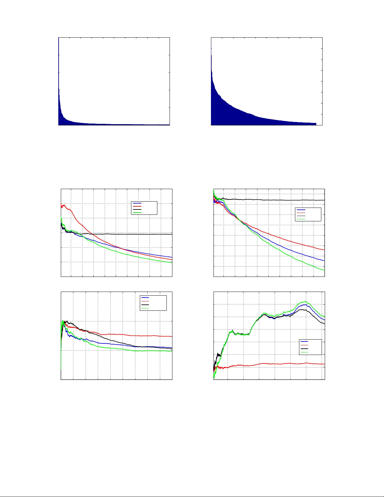
Graph Clustering Bandits f or Recommendation Shuai Li DiST A, Uni versity of Insubria, Italy shuaili.sli@gmail.com Claudio Gentile DiST A, Uni versity of Insubria, Italy claudio.gentile@uninsubria.it Alexandros Karatzoglou T elefonica Research, Spain alexk@tid.es May 3, 2016 Abstract W e in vestigate an efficient context-dependent clustering technique for recommender systems based on exploration-exploitation strategies through multi-armed bandits over multiple users. Our algorithm dynamically groups users based on their observed beha vioral similarity during a sequence of logged activities. In doing so, the algorithm reacts to the currently served user by shaping clusters around him/her but, at the same time, it explores the generation of clusters over users which are not currently engaged. W e moti vate the effecti veness of this clustering policy , and provide an extensi ve empirical analysis on real-world datasets, showing scalability and improv ed prediction performance over state-of- the-art methods for sequential clustering of users in multi-armed bandit scenarios. 1 Intr oduction Exploration-exploitation techniques a.k.a. Bandits are becoming an essential tool in modern recommenders systems [9, 12]. Most recommendation setting inv olve an e ver changing dynamic set of items, in man y domains such as news and ads recommendation the item set is changing so rapidly that is impossible to use standard collaborati ve filtering techniques. In these settings bandit algorithms such as contextual bandits hav e been pro ven to work well [10] since they provide a principled way to gauge the appeal of the new items. Y et, one drawback of contextual bandits is that they mainly work in a content-dependent regime, the user and item content features determine the preference scores so that any collaborativ e effects (joint user preferences ov er groups of items) that arise are being ignored. Incorporating collaborativ e effects into bandit algorithms can lead to a dramatic increase in the quality of recommendations. In bandit algorithms this has been mainly done by clustering the user . For instance, we may want to serve content to a group of users by taking adv antage of an underlying network of preference relationships among them. These preference relationships can either be e xplicitly encoded in a graph, where adjacent nodes/users are deemed similar to one another , or implicitly contained in the data, and giv en as the outcome of an inference process that recognizes similarities across users based on their past behavior . T o deal with this issue a new type of bandit algorithms has been dev eloped which work under the assumption that users can be grouped (or clustered) based on their selection of items e.g. [8, 11]. The main assumption is that users form a graph where the edges are constructed based on signals of similar preference (e.g. a number of similar item selections). By partitioning the graphs, one can find a coherent group of users with similar preference and online beha vior . While these algorithms hav e been prov en to perform 1 significantly better then classical contextual bandits, the y ”only” provide exploration on the set of items. For ne w users or users with sparse activity it is very dif ficult to find an accurate group assignment. This is a particularly important issue since most recommendation settings face unbalancedness of user activity le vels, that is, relati vely few users hav e very high activity while the vast majority of users hav e little to practically no acti vity at all (see Figure 2 in Section 4). In this work, we introduce a ne w bandit algorithm that adds an extra exploration component ov er the group of users. In addition to the standard exploration-exploitation strategy ov er items, this algorithm e x- plores different clustering assignments of new users and users with low activity . The experimental ev alua- tion on four real datasets against baselines and state-of-the-art methods confirm that the additional dynamic paradigm tends to translate into solid performance benefits. 2 Learning Setting As in pre vious work in this literature (e.g., [8, 4]), we assume that user behavior similarity is represented by an underlying (and unknown) clustering over the set of users. Specifically , if we let U = { 1 , . . . , n } be the set of n users, we assume U can be partitioned into a small number m of clusters U 1 , U 2 , . . . , U m , where m is expected to be much smaller than n . The meaning of this clustering is that users belonging to the same cluster U j tend to have similar behavior , while users lying in dif ferent clusters hav e significantly di verging behavior . Both the partition { U 1 , U 2 , . . . , U m } and the common user behavior within each cluster are unknown to the learning system, and hav e to be inferred on the fly based on past user activity . The above inference procedure has to be carried out within a sequential decision setting where the learn- ing system (henceforth “the learne”) has to continuously adapt to the newly received information provided by the users. T o this ef fect, the learning process is divided into a discrete sequence of rounds: in round t = 1 , 2 , . . . , the learner receiv es a user index i t ∈ U to serve content to. Notice that the user to serv e may change at ev ery round, though the same user can recur many times. The sequence { i t } is exogenously determined by the w ay users interact with the system, and is not under our control. In practice, very high un- balancedness lev els of user acti vity are often observed. Some users are very activ e, man y others are (almost) idle or newly registered users, and their preferences are either extremely sporadic or even do not exist [9]. Along with i t , the system recei ves in round t a set of feature vectors C i t = { x t, 1 , x t, 2 , . . . , x t,c t } ⊆ R d representing the content which is currently a vailable for recommendation to user i t . The learner picks some ¯ x t = x t,k t ∈ C i t to recommend to i t , and then observ es i t ’ s feedback in the form of a numerical payoff a t ∈ R . In this scenario, the learner’ s goal is to maximize its total payoff P T t =1 a t ov er a giv en number T of rounds. When the user feedback the learner observes is only the click/no-click behavior , the payof f a t can be naturally interpreted as a binary feedback, so that the quantity P T t =1 a t T becomes a click-through rate (CTR), where a t = 1 if the recommended item ¯ x t was clicked by user i t , and a t = 0 , otherwise. In our experiments (Section 4), when the data at our disposal only provide the payof f associated with the item recommended by the logged policy , CTR is our measure of prediction accuracy . On the other hand, when the data come with payoffs for all possible items in C i t , then our measure of choice will be the cumulativ e r e gr et of the learner , 1 defined as follo ws. Let a t,k be the payof f associated in the data at hand with item x t,k ∈ C i t . Then the regret r t of the learner at time t is the extent to which the payoff of 1 In fact, for the sake of clarity , our plots will actually display ratios of cumulati ve regrets and ratios of CTRs —see Section 4 for details. 2 the best choice in hindsight at user i t exceeds the payof f of the learner’ s choice, i.e., r t =  max k =1 ,...,c t a t,k  − a t,k t , and the cumulati ve regret is simply T X t =1 r t . Notice that the round- t regret r t refers to the behavior of the learner when predicting preferences of user i t , thus the cumulativ e regret takes into duly account the relati ve “importance” of users, as quantified by their acti vity lev el. The same claim also holds when measuring performance through CTR. 3 The Algorithm Our algorithm, called Graph Cluster of Bandits (GCLUB, see Figure 1), is a v ariant of the Cluster of Bandits (CLUB) algorithm originally introduced in [8]. W e first recall how CLUB works, point out its weakness, and then describe the changes that lead to the GCLUB algorithm. The CLUB algorithm maintains ov er time a partition of the set of users U in the form of connected components of an undirected graph G t = ( U , E t ) whose nodes are the users, and whose edges E t encode our current belief about user similarity . CLUB starts off from a randomly sparsified version of the com- plete graph (having O ( n log n ) edges instead of O ( n 2 ) ), and then progressiv ely deletes edges based on the feedback pro vided by the current user i t . Specifically , each node i of this graph hosts a linear function w i,t : x → w > i,t x which is meant to estimate the payof f user i would provide had item x been recom- mended to him/her . The hope is that this estimates gets better and better over time. When the current user is i t , it is only vector w i t ,t that is updated based on i t ’ s payoff signal, similar to a standard linear bandit algorithm (e.g., [2, 5, 1, 4]) operating on the context vectors contained in C i t . Ev ery user i ∈ U hosts such a linear bandit algorithm. The actual recommendation issued to i t within C i t is computed as follows. First, the connected component (or cluster) that i t belongs to is singled out (this is denoted by b j t in Figure 1). Then, a suitable aggregate prediction vector (denoted by ¯ w b j t ,t − 1 in Figure 1) is constructed which collects information from all uses in that connected component. The vector so computed is engaged in a standard upper confidence-based e xploration-exploitation tradef f to select the item ¯ x t ∈ C i t to recommend to user i t . Once i t ’ s payof f a t is receiv ed, w i t ,t − 1 gets updated to w i t ,t (through a t and ¯ x t ). In turn, this may change the current cluster structure, for if i t was formerly connected to, say , node ` and, as a consequence of the update w i t ,t − 1 → w i t ,t , vector w i t ,t is no longer close to w `,t − 1 , then this is taken as a good indication that i t and ` cannot belong to the same cluster , so that edge ( i t , ` ) gets deleted, and new clusters over users are possibly obtained. The main weakness of CLUB in shaping clusters is that when responding to the current user feedback, the algorithm operates only locally (i.e., in the neigborhood of i t ). While advantageous from a computational standpoint, in the long run this has the se vere drawback of ov erfocusing on the (typically few) very acti ve users; the algorithm is not responsi ve enough to those users on which not enough information has been gathered, either because they are not so activ e (typically , the majority of them) or because they are simply ne wly registered users. In other words, in order to make better recommendations it’ s worthy to discov er and capture the “niches” of user preferences as well. Since une ven acti vity lev els among users is a standard pattern when users are many (and this is the case with our data, too — see Section 4), GCLUB complements CLUB with a kind of stochastic exploration at the lev el of cluster shaping. In ev ery round t , GCLUB deletes edges in one of two ways: with independent high probability 1 − r > 1 / 2 , GCLUB operates on component b j t as in CLUB, while with low probability 3 r the algorithm picks a connected component uniformly at random among the av ailable ones at time t , and splits this component into two subcomponents by in v oking a fast graph clustering algorithm (thereby generating one more cluster). This stochastic choice is only made during an initial stage of learning (when t ≤ T / 10 in GCLUB’ s pseudocode), which we may think of as a cold start re gime for most of the users. The graph clustering algorithm we used in our experiments was implemented through the Gr aclus software package from the authors of [7, 6]. Because we are running it ov er a single connected component of an initially sparsified graph, this tool turned out to be quite fast in our e xperimentation. The rationale behind GCLUB is to add an extra layer of exploration-vs-exploitation tradeoff, which operates at the le vel of clusters. At this lev el, exploration corresponds to picking a cluster at random among the av ailable ones, while exploitation corresponds to working on the cluster the current user belongs to. In the absence of enough information about the current user and his/her neighborhood, exploring other clusters is intuiti vely beneficial. W e will see in the next section that this is indeed the case. 4 Experiments In this section, we briefly describe the setting and the outcome of our experimental in vestigation. 4.1 Datasets W e tested our algorithm on four freely av ailable real-world benchmark datasets against standard bandit baselines for multiple users. LastFM, Delicious, and Y ahoo datasets. For the sake of fair comparison, we carefully followed and implemented the experimental setup as described in [8] on these datasets, we refer the reader to that paper for details. The Y ahoo dataset is the one called “ Y ahoo 18k” therein. MovieLens dataset. This is the freely av ailable 2 benchmark dataset MovieLens 100k. In this dataset, there are 100 , 000 ratings from n = 943 users on 1682 movies, where each user has rated at least 20 movies. Each movie comes with a number of features, like id, movie title, release date, video release date, and genres. After some data cleaning, we extracted numerical features through a standard tf-idf procedure. W e then applied PCA to the resulting feature vectors so as to retain at least 95% of the original variance, gi ving rise to item vectors x t,k of dimension d = 19 . Finally , we normalized all features so as to have zero (empirical) mean and unit (empirical) variance. As for payoffs, we generated binary payoffs, by mapping any nonzero rating to payoff 1, and the zero rating to payoff 0. Moreover , for each timestamp in the dataset referring to user i t , we generated random item sets C i t of size c t = 25 for all t by putting into C i t an item for which i t provided a payoff of 1, and then picking the remaining 24 vectors at random from the av ailable movies up to that timestamp. Hence, each set C i t is likely to contain only one (or very few) movie(s) with payof f 1, out of 25. The total number of rounds was T = 100 , 000 . W e took the first 10 K rounds for parameter tuning, and the rest for testing. In Figure 2, we report the acti vity le vel of the users on the Y ahoo and the MovieLens datasets. As e vinced by these plots, 3 such lev els are quite div erse among users, and the emerging pattern is the same across these datasets: there are few v ery engaged users and a long tail of (almost) unengaged ones. 2 http://grouplens.org/datasets/mo vielens . 3 W ithout loss of generality , we take these two datasets to provide statistics, but similar shapes of the plots can be established for the other two datasets. 4 4.2 Algorithms W e compared GCLUB to three representativ e competitors: LinUCB-ONE, LinUCB-IND, and CLUB. LinUCB-ONE and LinUCB-IND are members of the LinUCB family of algorithms [2, 5, 1, 4] and are, in some sense, extreme solutions: LinUCB-ONE allocates a single instance of LinUCB across all users (thereby making the same prediction for all users – which would be effecti ve in a few-hits scenario), while LinUCB-IND (“LinUCB INDependent”) allocates an independent instance of LinUCB to each user , so as to provide personalized recommendations (which is likely to be effecti ve in the presence of many niches ). CLUB is the online clustering technique from [8]. On the Y ahoo dataset, we run the featureless version of the LinUCB-lik e algorithm in [4], i.e., a version of the UCB1 algorithm of [3]. The corresponding ONE and IND versions are denoted by UCB-ONE and UCB-IND, respecti vely . Finally , all algorithms ha ve also been compared to the tri vial baseline (denoted here as RAN) that selects the item within C i t fully at RANdom. W e tuned the parameters of the algorithms in the training set with a standard grid search as in [8], and used the test set to e valuate predictiv e performance. The training set was about 10% of the test set for all datasets, b ut for Y ahoo, where it turned out to be 4 around 6.2%. All e xperimental results reported here ha ve been av eraged ov er 5 runs (but in fact v ariance across these runs was fairly small). 4.3 Results Our results are summarized in Figure 3, where we report test set prediction performance. On LastFM, Delicious, and MovieLens, we measured the ratio of the cumulativ e regret of the algorithm to the cumulativ e regret of the random predictor RAN (so that the lower the better). On the Y ahoo dataset, because the only av ailable payof fs are those associated with the items recommended in the logs, we measured instead the ratio of Clickthrough Rate (CTR) of the algorithm to the CTR of RAN (so that the higher the better). Whereas all four datasets are generated by real online web applications, it is worth remarking that these datasets are indeed quite dif ferent in the way customers consume the associated content. For instance, the Y ahoo dataset is deri ved from the consumption of news that are often interesting for lar ge portions of users, hence there is no strong polarization into subcommunities (a typical “fe w hits” scenario). It is thus unsur- prising that on Y ahoo (Lin)UCB-ONE is already doing quite well. This also explains why (Lin)UCB-IND is so poor (almost as poor as RAN). At the other e xtreme lies Delicious, deri ved from a social bookmarking web service, which is a many niches scenario. Here LinUCB-ONE is clearly underperforming. On all these datasets, CLUB performs reasonably well (this is consistent with the findings in [8]), but in some cases the improvement ov er the best performer between (Lin)UCB-ONE and (Lin)UCB-IND is incremental. On LastFM, CLUB is e ven outperformed by LinUCB-IND in the long run. Finally , GCLUB tends to outperform all its competitors (CLUB included) in all cases. Though preliminary in nature, we belie ve these findings are suggestiv e of two phenomena: i. building clusters ov er users solely based on past user behavior can be beneficial; ii. in settings of highly diverse user engagement lev els (Figure 2), combining sequential clustering with a stochastic exploration mechanism operating at the le vel of cluster formation may enhance prediction performance e ven further . Refer ences [1] Y . Abbasi-Y adkori, D. P ´ al, and C. Szepesv ´ ari. Improv ed algorithms for linear stochastic bandits. Pr oc. NIPS , 2011. 4 Recall that on the Y ahoo dataset records are discarded on the fly , so training and test set sizes are not under our full control — see, e.g., [10, 8]. 5 [2] P . Auer . Using confidence bounds for exploration-exploitation trade-offs. J ournal of Machine Learning Resear ch , 3:397–422, 2002. [3] P . Auer , N. Cesa-Bianchi, and P . Fischer . Finite-time analysis of the multiarmed bandit problem. Machine Learning , 2001. [4] N. Cesa-Bianchi, C. Gentile, and G. Zappella. A gang of bandits. In Pr oc. NIPS , 2013. [5] W . Chu, L. Li, L. Reyzin, and R. E. Schapire. Contextual bandits with linear payof f functions. In Pr oc. AIST A TS , 2011. [6] I. Dhillon, Y . Guan, and B. Kulis. A fast kernel-based multile vel algorithm for graph clustering. In Pr oc. SIGKDD , 2005. [7] I. Dhillon, Y . Guan, and B. Kulis. W eighted graph cuts without eigenv ectors: A multilev el approach. In IEEE T ransactions on P attern Analysis and Machine Intelligence , 2007. [8] C. Gentile, S. Li, and G. Zappella. Online clustering of bandits. In Pr oc. ICML , 2014. [9] A. Lacerda, A. V eloso, and N. Zi viani. Exploratory and interactiv e daily deals recommendation. In Pr oc. RecSys , 2013. [10] L. Li, W . Chu, J. Langford, and R. Schapire. A conte xtual-bandit approach to personalized news article recommendation. In Pr oc. WWW , pages 661–670, 2010. [11] T . T . Nguyen and H. W . Lauw . Dynamic clustering of contextual multi-armed bandits. In Pr oc. CIKM , 2014. [12] L. T ang, Y . Jiang, L. Li, and T . Li. Ensemble contextual bandits for personalized recommendation. In Pr oc. RecSys , 2014. 6 Input : Exploration parameter α > 0 ; cluster exploration probability r < 1 / 2 . Init : • b i, 0 = 0 ∈ R d and M i, 0 = I ∈ R d × d , i = 1 , . . . n ; • Clusters ˆ U 1 , 1 = U , number of clusters m 1 = 1 ; • Graph G 1 = ( U , E 1 ) , G 1 has O ( n log n ) edges and is connected. for t = 1 , 2 , . . . , T do Receiv e i t ∈ U ; Set w i,t − 1 = M − 1 i,t − 1 b i,t − 1 , i = 1 , . . . , n ; Get item set C i t = { x t, 1 , . . . , x t,c t } ; Determine b j t ∈ { 1 , . . . , m t } such that i t ∈ ˆ U b j t ,t , and set ¯ M b j t ,t − 1 = I + X i ∈ ˆ U b j t ,t ( M i,t − 1 − I ) , ¯ b b j t ,t − 1 = X i ∈ ˆ U b j t ,t b i,t − 1 , ¯ w b j t ,t − 1 = ¯ M − 1 b j t ,t − 1 ¯ b b j t ,t − 1 ; Set k t = argmax k =1 ,...,c t  ¯ w > b j t ,t − 1 x t,k + C B b j t ,t − 1 ( x t,k )  , where C B b j t ,t − 1 ( x ) = α q x > ¯ M − 1 b j t ,t − 1 x log( t + 1) . Observe payof f a t ∈ [ − 1 , 1] ; Let ¯ x t = x t,k t ; Update weights: • M i t ,t = M i t ,t − 1 + ¯ x t ¯ x > t , • b i t ,t = b i t ,t − 1 + a t ¯ x t , • Set M i,t = M i,t − 1 , b i,t = b i,t − 1 for all i 6 = i t ; Update clusters: • Flip independent coin X t ∈ { 0 , 1 } with P ( X t = 1) = r . – If X t = 0 then delete from E t all ( i t , ` ) such that || w i t ,t − 1 − w `,t − 1 || > f C B i t ,t − 1 + f C B `,t − 1 , f C B i,t − 1 = α s 1 + log(1 + T i,t − 1 ) 1 + T i,t − 1 , T i,t − 1 = |{ s ≤ t − 1 : i s = i }| , i ∈ U ; – If X t = 1 and t ≤ T / 10 then pick at random index j ∈ { 1 , . . . , m t } , j 6 = b j t , and split ˆ U j,t into tw o subclusters ˆ U j,t, 1 and ˆ U j,t, 2 by means of a standard graph clustering procedure. Delete all edges between ˆ U j,t, 1 and ˆ U j,t, 2 . • Let E t +1 be the resulting set of edges, set G t +1 = ( U , E t +1 ) , and compute associated clusters ˆ U 1 ,t +1 , ˆ U 2 ,t +1 , . . . , ˆ U m t +1 ,t +1 . end for Figure 1: Pseudocode of the GCLUB algorithm. 7 0 200 400 600 800 1000 1200 1400 1600 1800 2000 0 0.5 1 1.5 2 2.5 x 10 4 User Count Yahoo 0 100 200 300 400 500 600 700 800 900 1000 0 100 200 300 400 500 600 700 800 User Count MovieLens Figure 2: User activity levels on the Y ahoo (left) and the MovieLens (right) datasets. Users are sorted in decreasing order according to the number of times they provide feedback to the learning system. For the sake of better visibility , on the Y ahoo dataset we truncated to the 2K most activ e users (out of 18K). 1 2 3 4 5 6 7 8 9 10 x 10 4 0.7 0.75 0.8 0.85 0.9 0.95 1 Rounds Cum. Regr. of Alg. / Cum. Regr. of RAN LastFM 100k CLUB LinUCB−IND LinUCB−ONE GCLUB 1 2 3 4 5 6 7 8 9 10 x 10 4 0.84 0.86 0.88 0.9 0.92 0.94 0.96 0.98 1 Rounds Cum. Regr. of Alg. / Cum. Regr. of RAN Delicious 100k CLUB LinUCB−IND LinUCB−ONE GCLUB 0 1 2 3 4 5 6 7 8 x 10 4 0.9 0.95 1 1.05 Rounds Cum. Regr. of Alg. / Cum. Regr. of RAN MovieLens 100k CLUB LINUCB−IND LINUCB−ONE GCLUB 1 2 3 4 5 6 7 x 10 4 0.5 1 1.5 2 2.5 3 3.5 4 Rounds CTR of Alg. / CTR of RAN Yahoo! 18k CLUB UCB−IND UCB−ONE GCLUB Figure 3: Results on the LastFM (top left), the Delicious (top right), MovieLens (bottom left), and the Y ahoo (bottom right) datasets. On the first three plots, we display the time ev olution of the ratio of the cumulativ e regret of the algorithm (“ Alg”) to the cumulativ e regret of RAN, where “ Alg” is either “GCLUB” (green), CLUB (blue), “LinUCB-IND” (red), or “LinUCB-ONE” (black). On the Y ahoo dataset, we instead plot the ratio of Clickthrough Rate (CTR) of “ Alg” to the Clickthrough Rate of RAN. Colors are consistent throughout the four plots. 8