Robust Probability Updating

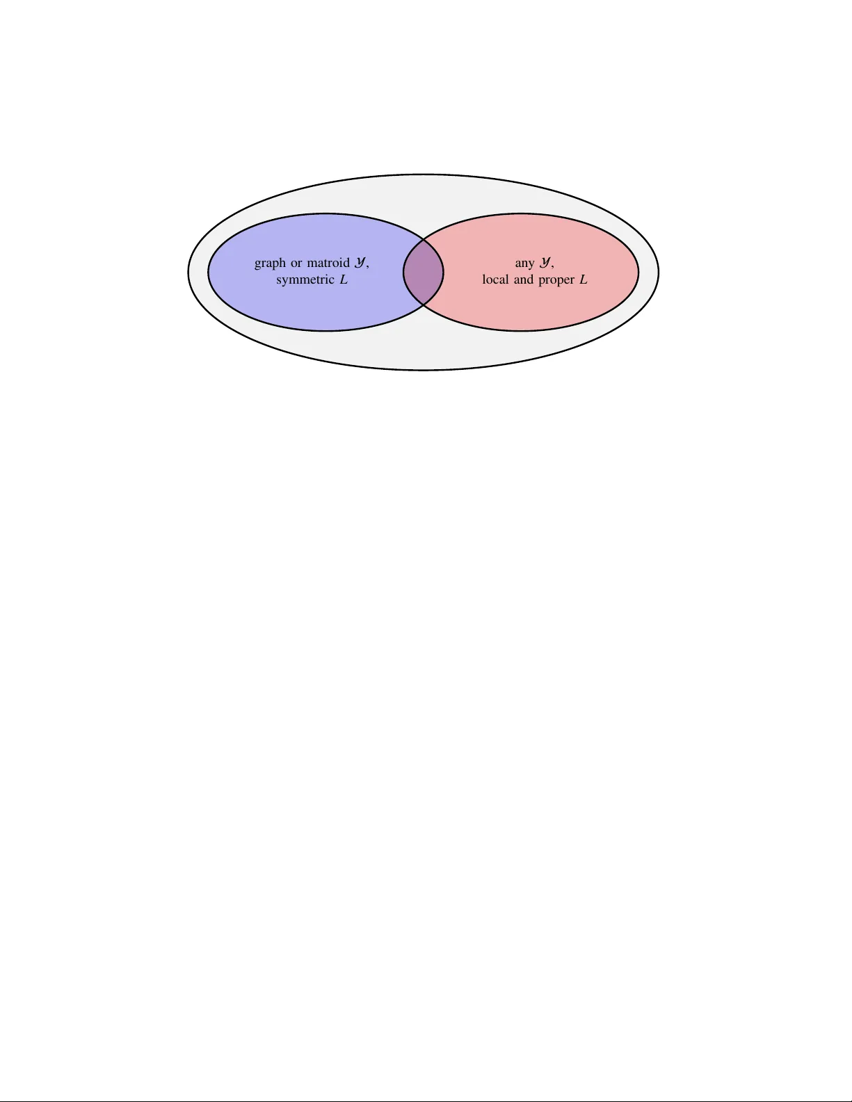
Rob ust Probability Updating I Thijs van Ommen a, ∗ , W outer M. K oolen b , Thijs E. Feenstra c , Peter D. Gr ¨ unwald b,c a Universiteit van Amster dam, Science P ark 904, 1098 XH Amsterdam, The Netherlands b Centrum W iskunde & Informatica, Science P ark 123, 1098 XG Amsterdam, The Netherlands c Universiteit Leiden, Niels Bohrwe g 1, 2333 CA Leiden, The Netherlands Abstract This paper discusses an alternati ve to conditioning that may be used when the probabil- ity distribution is not fully speciﬁed. It does not require any assumptions (such as CAR: coarsening at random) on the unknown distribution. The well-known Monty Hall prob- lem is the simplest scenario where neither naiv e conditioning nor the CAR assumption su ﬃ ce to determine an updated probability distribution. This paper thus addresses a generalization of that problem to arbitrary distrib utions on ﬁnite outcome spaces, arbi- trary sets of ‘messages’, and (almost) arbitrary loss functions, and provides existence and characterization theorems for robust probability updating strategies. W e ﬁnd that for logarithmic loss, optimality is characterized by an ele gant condition, which we call RCAR (re verse coarsening at random) . Under certain conditions, the same condition also characterizes optimality for a much larger class of loss functions, and we obtain an objective and general answer to how one should update probabilities in the light of new information. K e ywor ds: probability updating, maximum entropy, loss functions, minimax decision making 1. Introduction There are many situations in which a decision maker receiv es incomplete data and still has to reach conclusions about these data. One type of incomplete data is coarse data: instead of the real outcome of a random e vent, the decision maker observes a subset of the possible outcomes, and kno ws only that the actual outcome is an element of this subset. An example frequently occurs in questionnaires, where people may be asked if their date of birth lies between 1950 and 1960 or between 1960 and 1970 et cetera. Their exact year of birth is unkno wn to us, but at least we no w know for sure in which decade they are born. W e introduce a simple and concrete motiv ating instance of coarse data with the following e xample. I This work is adapted from dissertation [1, Chapters 6 and 7], which extends MSc. thesis [2]. ∗ Corresponding author Email addr esses: T.vanOmmen@uva.nl (Thijs van Ommen), wmkoolen@cwi.nl (W outer M. K oolen), pdg@cwi.nl (Peter D. Gr ¨ unwald) © 2016. This accepted manuscript is made available under the CC-BY -NC-ND 4.0 licence: http: // creativecommons. org/ licenses/ by- nc- nd/ 4. 0/ . Published in International Journal of Appr ox- imate Reasoning (2016) pp. 30–57, http: // dx. doi. org/ 10. 1016/ j. ijar. 2016. 03. 001 Example A (Fair die) . Suppose I thro w a fair die. I get to see the result of the throw , but you do not. Now I tell you that the result lies in the set { 1 , 2 , 3 , 4 } . This is an example of coarse data. Y ou kno w that I used a fair die and that what I tell you is true. Now you are asked to gi ve the probability that I rolled a 3. Likely , you would say that the probability of each of the remaining possible results is 1 / 4. This is the knee-jerk reaction of someone who studied probability theory , since this is standard conditioning . But is this always correct? Suppose that there is only one alternati ve set of results I could gi ve you after rolling the die, namely the set { 3 , 4 , 5 , 6 } . I can now follow a coarsening mechanism : a pro- cedure that tells me which subset to reveal gi ven a particular result of the die roll. If the outcome is 1, 2, 5, or 6, there is nothing for me to choose. Suppose that if the out- come is 3 or 4, the coarsening mechanism I use selects set { 1 , 2 , 3 , 4 } or set { 3 , 4 , 5 , 6 } at random, each with probability 1 / 2. If I throw the die 6000 times, I expect to see the outcome 3 a thousand times. Therefore I expect to report the set { 1 , 2 , 3 , 4 } ﬁv e hun- dred times after I see the outcome 3. It is clear that I expect to report the set { 1 , 2 , 3 , 4 } 3000 times in total. So for die rolls where I told you { 1 , 2 , 3 , 4 } , the probability of the true outcome being 3 is actually 1 / 6 with this coarsening mechanism. W e see that the prediction of 1 / 4 from the ﬁrst paragraph was not correct, in the sense that the prob- abilities computed there do not correspond to the long-run relati ve frequencies. W e conclude that the knee-jerk reaction is not always correct. In Example A we hav e seen that standard conditioning does not alw ays give the correct answers. Heitjan and Rubin [3] answer the question under what circumstances standard conditioning of coarse data is correct. They discovered a necessary and suf- ﬁcient condition of the coarsening mechanism, called coarsening at random (CAR) . A coarsening mechanism satisﬁes the CAR condition if, for each subset y of the out- comes, the probability of choosing to report y is the same no matter which outcome x ∈ y is the true outcome. It depends on the arrangement of possible re vealed subsets whether a coarsening mechanism e xists that satisﬁes CAR. It holds automatically if the subsets that can be rev ealed partition the sample space. As noted by Gr ¨ unwald and Halpern [4] howe ver , as soon as events ov erlap, there exist distributions on the space for which CAR does not hold. In many such situations it e ven cannot hold; see Gill and Gr ¨ unwald [5] for a complete characterization of the — quite restricted — set of situ- ations in which CAR can hold. No coarsening mechanism satisﬁes the CAR condition for Example A. W e hasten to add that we neither question the validity of conditioning nor do we want to replace it by something else. The real problem lies not with conditioning, but with conditioning within the wrong sample space, in which the coarsening mechanism cannot be represented. If we had a distribution P on the correct, larger space, which allows for statements like ‘the probability is α that I choose { 1 , 2 , 3 , 4 } to rev eal if the outcome is 3’, then conditioning would give the correct results. The problem with coarse data is though that we often do not have enough information to identify P — e.g. we do not know the v alue of α and do not want to assume that it is 1 / 2. Hence- forth, we shall refer to conditioning in the ov erly simple space as ‘naiv e conditioning’. In this paper we propose update rules for situations in which naiv e conditioning gi ves the wrong answer , and conditioning in the right space is problematic because the un- 2 derlying distribution is partially unknown. These are in variably situations in which tw o or more of the potentially observed e vents ov erlap. W e illustrate this further with a famously counter-intuiti ve example: the Monty Hall puzzle, posed by Selvin [6] and popularized years later in Ask Marilyn, a weekly column in Parade Magazine by Marilyn v os Sav ant [7]. Example B (Monty Hall) . Suppose you are on a game show and you may choose one of three doors. Behind one of the doors a car can be found, but the other two only hide a goat. Initially the car is equally likely to be behind each of the doors. After you hav e picked one of the doors, the host Monty Hall, who knows the location of the prize, will open one of the other doors, rev ealing a goat. Now you are asked if you would like to switch from the door you chose to the other unopened door . Is it a good idea to switch? At this moment we will not answer this question, but we show that the problem of choosing whether to switch doors is an e xample of the coarse data problem. The unknown random value we are interested in is the location of the car: one of the three doors. When the host opens a door di ﬀ erent from the one you picked, re vealing a goat, this is equiv alent to reporting a subset. The subset he reports is the set of the two doors that are still closed. For example, if he opens door 2, this tells us that the true value, the location of the car, is in the subset { 1 , 3 } . Note that if you hav e by chance picked the correct door, there are tw o possible doors Monty Hall can open, so also two subsets he can report. This implies that Monty has a choice in reporting a subset. How does Monty’ s coarsening mechanism inﬂuence your prediction of the true location of the car? The CAR condition can only be satisﬁed for very particular distributions of where the prize is: the probability that the prize is hidden behind the initially chosen door must be either 0 or 1, otherwise no CAR coarsening mechanism exists [4, Example 3.3] 1 . If the prize is hidden in any other way , for example uniformly at random as we assume, then CAR cannot hold, and naiv e conditioning will result in an incorrect conclusion for at least one of the two subsets. Examples A and B are just two instances of a more general problem: the number of outcomes may be arbitrary; the initial distrib ution of the true outcome may be any dis- tribution; and the subsets of outcomes that may be reported to the decision maker may be any family of sets. Our goal is to deﬁne general procedures that tell us how to update the probabilities of the outcomes after making a coarse observation, in such situations where naiv e conditioning is not adequate. W e are aiming for modular methods that do not enforce a particular interpretation of probability . In Example A, we saw “object- iv e” probabilities: the original distributions were kno wn, and the updated probabilities we found could again be interpreted as frequencies over many repetitions of the same experiment. The original distribution of the outcomes could howe ver also express a subjectiv e prior belief of how likely each outcome is. For example, in Example B, the uniform distribution of the location of the car requires an assumption on the frequent- 1 This uses the weak version of CAR in the terminology of Jaeger [8], in which outcomes with probability 0 are e xempt from the equality constraint. A strong CAR coarsening mechanism does not e xist regardless of the probabilities with which the prize is hidden. 3 ist’ s part, while it may be a reasonable choice of prior for a subjective Bayesian [9]. In this case, the updated probabilities after a coarse observation take the role of the Bayesian posterior distrib ution. In any case, we will refer to the initial probability of an outcome, regardless of observ ations, as the mar ginal probability . W ithout any assumptions on the quizmaster’ s strategy (i.e. the coarsening mech- anism), the conditional distributions of outcomes gi ven observ ations will be unknown, and this uncertainty cannot be fully expressed by a single probability distrib ution over the outcomes. One way to deal with this is by means of imprecise probability , i.e. by explicitly tracking all possible quizmaster strategies and their e ﬀ ects [10]. W e ho wever focus on obtaining a single (precise) updated probability . T o get such a single answer , we could make some assumption about ho w the quizmaster chooses his strategy . As- suming that the coarsening mechanism satisﬁes CAR is one such approach, but as we saw in the two examples, there are scenarios where this assumption cannot hold. W e instead take a worst-case appr oach , treating the coarsening of the observation and the subsequent probability update as a game between two players: the quizmaster and the contestant (named for their roles in the Monty Hall scenario). The subset of outcomes communicated by the quizmaster to the contestant will be called the message . In this ﬁctional game, the quizmaster’ s goal is the opposite of the contestant’ s, namely to mak e predicting the true outcome as hard as possible for the contestant. This type of zero-sum game, in which some information is revealed to the contestant was also considered by Gr ¨ unwald and Halpern [11] and Ozdenoren and Peck [12]. Such situations are rare in practice: The sender of a message might be moti vated by interests other than informing us (for example, a ne wspaper may be trying to optimize its sales ﬁgures, or a compan y may want to present its performance in the best light), b ut rarely by trying to be as uninformati ve as possible (though see Section 5.5, where we consider the case that the players’ goals are not diametrically opposed). In other situations, the ‘sender’ might not be a rational being at all, but just some unknown process. Y et this game is a useful way to look at the problem of updating our probabilities even if we do not believ e that the coarsening mechanism is chosen adversarially: if we simply do not know how ‘nature’ chooses which message to gi ve us and do not want to make any assumptions about this, then choosing the worst-case (or minimax ) optimal probability update as deﬁned here guarantees that we incur at most some ﬁxed expected loss, while any other probability update may lead to a larger expected loss depending on the unknown coarsening mechanism. While from a Bayesian point of vie w , such a choice might at ﬁrst seem ov erly pessimistic, we note that in all cases we consider , our approach is fully consistent with a Bayesian one — our results can be interpreted as recommending a certain prior on the quizmaster’ s assignment of messages to outcomes, which in simple cases (such as Monty Hall) coincides with a prior that Bayesians would be tempted to adopt as well. W e will employ a loss function to measure how well the quizmaster and the contest- ant are doing at this game. Our results apply to a wide v ariety of loss functions. For an analysis of the Monty Hall g ame, 0-1 loss would be appropriate, as the contestant must choose a single door; this is the approach used by Gill [9] and Gnedin [13]. Other loss functions, such as logarithmic loss and Brier loss (see e.g. Gr ¨ unwald and Dawid [14]), also allow the contestant to formulate their prediction of where the prize is hidden as an arbitrary probability distribution o ver the outcomes. 4 W e model probability updating as a game as follows. An outcome x is drawn with known marginal probability p x and shown to the quizmaster , who picks a consistent message y 3 x using his coarsening mechanism P ( y | x ). Seeing only y , the contestant makes a prediction in the form of a probability mass function Q ( · | y ) on outcomes. Then x is revealed and the prediction quality measured using the loss function L . The quizmaster / contestant aim to maximize / minimize the expected loss X x p x X y 3 x P ( y | x ) L  x , Q ( · | y )  . (1) For the Monty Hall game with logarithmic or Brier , i.e. squared loss, the worst-case optimal answer for the contestant is to put probability 1 / 3 on his initially chosen door and 2 / 3 on the other door . (These probabilities agree with the literature on the Monty Hall game.) Surprisingly , we will see (in Example D on page 17) that for very similar games, logarithmic and Brier loss may lead to two di ﬀ erent answers! W e will ﬁnd that for ﬁnite outcome spaces, both players in our game have worst- case optimal strategies for many loss functions: the quizmaster has a strategy that makes the contestant’ s prediction task as hard as possible, and the contestant has a strat- egy that is guaranteed to gi ve good predictions no matter ho w the quizmaster coarsens. W e gi ve characterizations that allow us to recognize such strategies, for di ﬀ erent con- ditions on the loss functions. Example A (continued). For logarithmic loss, the worst-case optimal prediction of the die roll conditional on the rev ealed subset is found with the help of Theorem 10. The worst-case optimal prediction giv en that you observe the set { 1 , 2 , 3 , 4 } is: predict outcomes 1 and 2 each with probability 1 / 3, and predict 3 and 4 each with probability 1 / 6. Symmetrically , giv en that you observe the set { 3 , 4 , 5 , 6 } , the worst-case optimal prediction is: 3 and 4 with probability 1 / 6, and 5 and 6 with probability 1 / 3. These probabilities correspond with the uniform coarsening mechanism giv en ear- lier . Howe ver , it is a good prediction ev en if you do not know what coarsening mech- anism I am using. An intuitiv e argument for this is the follo wing: If I wanted, I could use a very e xtreme coarsening mechanism, al ways choosing to rev eal the set { 1 , 2 , 3 , 4 } when the die comes up 3 or 4. But this is balanced by the possibility that I might be us- ing the opposite coarsening mechanism, which always rev eals { 3 , 4 , 5 , 6 } if the result is 3 or 4. The worst-case optimal prediction gi ven above hedges against both possibilities. 1.1. Overview of contents In Section 2, we will giv e a precise deﬁnition of the ‘conditioning game’ we de- scribed. In Section 3, we ﬁnd general conditions on the loss function under which worst-case optimal strategies for the quizmaster and contestant exist, and we charac- terize such strategies. (See Figure 3 for a visual illustration of the concepts used in this section.) If stronger conditions hold, worst-case optimal strategies for both play- ers may be easier to recognize. This is explored for two classes of loss functions in Section 4; in particular , we ﬁnd that for local proper loss functions (among which loga- rithmic loss), worst-case optimal strategies for the quizmaster are characterized by a simple condition on their probabilities that we call the RCAR (r everse CAR) condition. RCAR bears a striking similarity to CAR, but with the roles of outcomes and messages 5 graph or matroid Y , symmetric L an y Y , local and proper L RCAR Figure 1: Classes of games for which the RCAR condition characterizes optimality . Y is the set of messages and L is the loss function. interchanged. Also, by Lemma 14, if a betting game is played repeatedly and the con- testant is allowed to distribute in vestments over di ﬀ erent outcomes and to rein vest all capital gained so far in each round, then the same strategy is optimal, r egar dless of the pay-o ﬀ s! An overvie w of the theorems and the conditions under which they apply is giv en in T able 1 on page 13. Then in Section 5 we look at the inﬂuence of the set of av ailable messages, im- posing only the minimal symmetry requirement on the loss function. W e prov e that for graph and matroid games (and only these) the optimality condition is again RCAR. As RCAR is independent of the loss function, for such games probability updating can hence be meaningfully deﬁned and performed completely agnostic of the task at hand. Many examples are included to illustrate (the limits of) the theoretical results. Section 6 giv es some concluding remarks. An ov erview of the results in this work is presented in Figure 1. All proofs are given in Appendix A. Highlight. A central feature of probability distributions is that they summarize what a decision maker would do under a v ariety of circumstances (loss functions): for each particular loss function the decision maker minimizes expected loss (maximizes util- ity) using the same distrib ution no matter what speciﬁc loss function is used. Since we generalize conditioning by using a minimax approach, one might e xpect that for di ﬀ er- ent loss functions one ends up with di ﬀ erent updated probabilities. Still, we show that for a rich selection of scenarios optimality is characterized by the RCAR condition, which is independent of the loss function. As a result, our updated probabilities are application-independent , and we may hence think of them — if we are willing to take a cautious (minimax) approach — as expressing what an experimenter should believe after having recei ved the data. W e isolate two distinct classes of scenarios where such application independence obtains. First, games with graph and matroid message sets (e xtending Monty Hall) and symmetric loss functions. Second, graphs with arbitrary message sets and proper local loss functions, including the symmetric logarithmic loss as well as its asymmetric gen- eralizations appropriate for Kelly gambling with arbitrary payo ﬀ s. In these scenarios 6 our application-independent update rule has an objecti ve appeal, and we feel that its importance may transcend that of being “merely” minimax optimal. This work is an extension of Feenstra [2] to loss functions other than logarithmic loss, and to the case where the worst-case optimal strategy for the quizmaster assigns prob- ability 0 to some combinations of outcomes x and messages y with x ∈ y . It can also be seen as a concrete application of the ideas in Gr ¨ unwald and Da wid [14] about minimax optimal decision making and its relation to entropy . A more extensi ve discussion of worst-case optimal probability updating can be found in V an Ommen [1]; in particular , there the question of e ﬃ cient algorithms for determining w orst-case optimal strategies is also considered. 2. Deﬁnitions and problem f ormulation A (pr obability updating) game G is deﬁned as a quadruple ( X , Y , p , L ), where X is a ﬁnite set, Y is a family of distinct subsets of X with S y ∈Y y = X , p is a strictly positiv e probability mass function on X , and L is a function L : X × ∆ X → [0 , ∞ ], where ∆ X is the set of all probability mass functions on X . W e call X the outcome space , Y the message structure , p the marginal distribution , and L the loss function . It is clear that outcomes with zero marginal probability p do not contribute to the objectiv e (1), so we may exclude them without loss of generality . Let us illustrate these deﬁnitions by applying them to our example. Example B (continued). W e assume the car is hidden uniformly at random behind one of the three doors. W ith this assumption, we can abstract a way the initial choice of a door by the contestant: by symmetry , we can assume without loss of generality that he always picks door 2. Then the probability updating game starts with the quizmaster opening door 1 or 3, thereby giving the message “the car is behind door 2 or 3” or “the car is behind door 1 or 2”, respectively . This can be expressed as follows in our formalization: • outcome space X = { x 1 , x 2 , x 3 } ; • message space Y = { y 1 , y 2 } with y 1 = { x 1 , x 2 } and y 2 = { x 2 , x 3 } ; • marginal distrib ution p uniform on X . If a loss function L is also giv en, this fully speciﬁes a game. One example is random- ized 0-1 loss, which is giv en by L ( x , Q ) = 1 − Q ( x ). Here x is the true outcome, and Q is the contestant’ s prediction of the true outcome in the form of a probability distrib ution. Thus the prediction Q is awarded a smaller loss if it assigned a larger probability Q ( x ) to the outcome x that actually obtained. W e will see other examples of loss functions in Section 2.2. A function from some ﬁnite set S to the reals R = ( −∞ , ∞ ) corresponds to an | S | - dimensional v ector when we ﬁx an order on the elements of S . W e write R S for the set of such functions / vectors. Even if no order on S is speciﬁed, this allows us to apply concepts from linear algebra to R S without ambiguity . For example, we may say that 7 some set is an a ﬃ ne subspace of R S . (This identiﬁcation and the resulting notation are also used by Schrijver [15].) Using this correspondence, we identify the elements of ∆ X with the |X| -dimensional vectors in the unit simplex, though we use ordinary function notation P ( x ) for its ele- ments. The probability mass function p that is part of a game’ s deﬁnition is also a vector in ∆ X . V ector notation p x will be used to refer to its elements to set p apart from P , which will denote distributions chosen by the quizmaster rather than ﬁxed by the game. For any message y ⊆ X , we deﬁne ∆ y = { P ∈ ∆ X | P ( x ) = 0 for x < y } . Note that these are vectors of the same length as those in ∆ X , though contained within a lower -dimensional a ﬃ ne subspace. A loss function L is called pr oper if P ∈ arg min Q ∈ ∆ X E X ∼ P L ( X , Q ) for all P ∈ ∆ X , and strictly pr oper if this minimizer is unique (this is standard terminology; see for instance Gneiting and Raftery [16]). Thus if a predicting agent belie ves the true distribution of an outcome to be gi ven by some P , such a loss function will encourage him to report Q = P as his prediction. 2.1. Strate gies Strategies for the players are speciﬁed by conditional distributions: a strategy P for the quizmaster consists of distributions on Y , one for each possible x ∈ X , and a strategy Q for the contestant consists of distributions on X , one for each possible y ∈ Y . These strategies deﬁne how the two players act in any situation: the quizmaster’ s strategy deﬁnes ho w he chooses a message containing the true outcome (the coarsening mechanism), and the contestant’ s strategy deﬁnes his prediction for each message he might receiv e. W e write P ( · | x ) for the distrib ution on Y the quizmaster plays when the true outcome is x ∈ X . Because p x > 0, this conditional distribution can be reco vered from the joint P ( x , y ) : = P ( y | x ) p x ; we will use this joint distribution to specify a strategy for the quizmaster . If P ( y ) : = P x ∈ y P ( x , y ) > 0, we may also write P ( · | y ) for the vector in ∆ y giv en by P ( x | y ) : = P ( x , y ) / P ( y ). No such rewrites can be made for Q , as no marginal Q ( y ) is speciﬁed by the game or by the strategy Q . T o shorten notation and to emphasize that Q is not a joint distribution, we write Q | y rather than Q ( · | y ) for the distribution that the contestant plays in response to message y . W e restrict the quizmaster to conditional distributions P for which P ( y | x ) = 0 if x < y ; that is, he may not ‘lie’ to the contestant. W e make no similar requirement on the contestant’ s choice of Q , though for proper loss functions, and in fact all other loss functions we will consider in our e xamples, the contestant can gain nothing from using a strategy Q for which Q | y ( x ) > 0 where x < y . P x 1 x 2 x 3 y 1 1 / 3 1 / 6 − y 2 − 1 / 6 1 / 3 p x 1 / 3 1 / 3 1 / 3 (2) Example B (continued). The table to the right spe- ciﬁes all aspects of a game except for its loss function: its outcome space (here, for the Monty Hall game, X = { x 1 , x 2 , x 3 } ), message space ( Y = { y 1 , y 2 } with y 1 = { x 1 , x 2 } and y 2 = { x 2 , x 3 } ) and marginal distribu- tion ( p uniform on X ). In this table we ha ve ﬁlled in a strategy P for the quizmaster in 8 the form of a joint distribution on pairs of x and y . The cells in the table where x < y are marked with a dash to indicate that P may not assign positiv e probability there. The probabilities in each column sum to the marginal probabilities at the bottom, so this joint distribution P has the correct marginal distribution on the outcomes. For this particular strategy , if the true outcome is x 2 , the quizmaster will giv e message y 1 or y 2 to the contestant with equal probability . More formally , write R ( X , Y ) as an abbreviation for the set of pairs { ( x , y ) | y ∈ Y , x ∈ y } . In the case of the Monty Hall game, there are four such pairs: R ( X , Y ) = { ( x 1 , y 1 ) , ( x 2 , y 1 ) , ( x 2 , y 2 ) , ( x 3 , y 2 ) } . The notation R R ( X , Y ) ≥ 0 represents the set of all func- tions from R ( X , Y ) to R ≥ 0 . If P is an element of this set and ( x , y ) ∈ R ( X , Y ), the value of P at ( x , y ) is denoted by P ( x , y ). For ( x , y ) with x < y , the notation P ( x , y ) does not correspond to a value of the function, b ut is taken to be 0. W e again identify the elements of R R ( X , Y ) ≥ 0 with vectors. Thus the mass function P shown in (2) is identiﬁed with a four -element v ector ( 1 / 3 , 1 / 6 , 1 / 6 , 1 / 3 ). (W e could have chosen a di ﬀ erent ordering instead.) W e deﬁne the set P of strate gies for the quizmaster as { P ∈ R R ( X , Y ) ≥ 0 | P y 3 x P ( x , y ) = p x for all x } ; this is a con vex set. The set of strategies for the contestant is Q : = ∆ Y X = { ( Q | y ) y ∈Y | Q | y ∈ ∆ X for each y ∈ Y } . For gi ven strategies P and Q , the expected loss the contestant incurs (1) is X x ∈X p x X y ∈Y : x ∈ y P ( y | x ) L ( x , Q | y ) = E X ∼ p E Y ∼ P ( ·| X ) L ( X , Q | Y ) = E ( X , Y ) ∼ P L ( X , Q | Y ) . (3) W e allow L to take the value ∞ ; if this value occurs with positiv e probability , then the contestant’ s expected loss is inﬁnite. Ho wev er , for terms where the probability is zero, we deﬁne 0 · ∞ = 0, as is consistent with measure-theoretic probability . W e model the probability updating problem as a zero-sum game between two play- ers with objective (3): the quizmaster chooses P ∈ P to maximize (3), while simul- taneously (that is, without kno wing P ) the contestant chooses Q ∈ Q to minimize that quantity . The game ( X , Y , p , L ) is common knowledge for the tw o players. If the contestant knew the quizmaster’ s strategy , he would pick a strategy Q that for each y minimizes the expected loss of predicting x giv en y . When the contestant receiv es a message and knows the distrib ution P ∈ ∆ X ov er the outcomes giv en that message, this expected loss is written as H L ( P ) : = inf Q ∈ ∆ X X x P ( x ) L ( x , Q ) = inf Q ∈ ∆ X E X ∼ P L ( X , Q ) . (4) This is the generalized entr opy of P for loss function L [14]. (Note that in the preceding display , P and Q are not strategies but simply distributions ov er X .) If the contestant picks his strategy Q this way , (3) becomes the expected generalized entr opy of the quizmaster’ s strategy P ∈ P : X y ∈Y P ( y ) H L ( P ( · | y )) , (5) where we again deﬁne terms with P ( y ) = 0 as 0. W e say a strategy P is worst-case optimal for the quizmaster if it maximizes this expected generalized entropy over all 9 P ∈ P . W e call the version of the game where the quizmaster has to play ﬁrst the maximin game, where the order of the words ‘max’ and ‘min’ reﬂects the order in which they appear in the expression for the value of this game as well as the order in which the maximizing and minimizing players take their turns. Similarly , if the contestant were to play ﬁrst (the minimax g ame), his goal might be to ﬁnd a strategy Q that minimizes his worst-case expected loss max P ∈P X x ∈ y P ( x , y ) L ( x , Q | y ) = max P ∈P E ( X , Y ) ∼ P L ( X , Q | Y ) . (6) (In this case, the maximum is always achie ved so we can write max rather than sup: for each x , the quizmaster can choose P that puts all mass on a y 3 x with the max- imum loss.) W e call a strategy worst-case optimal for the contestant if it achiev es the minimum of (6). It is an elementary result from game theory that if worst-case optimal strate gies P ∗ and Q ∗ exist for the two players, their e xpected losses are related by X y ∈Y P ∗ ( y ) H L ( P ∗ ( · | y )) ≤ max P ∈P X x ∈ y P ( x , y ) L ( x , Q ∗ | y ) (7) [17, Lemma 36.1: “maximin ≤ minimax”]. The inequality expresses that in a sequen- tial game where one of the players kno ws the other’ s strategy before choosing his o wn, the player to mov e second may have an adv antage. In the ne xt section, we will see that in many probability updating games, worst-case optimal strategies for both players exist (but may not be unique), and the maximum expected generalized entropy equals the minimum w orst-case expected loss: X y ∈Y P ∗ ( y ) H L ( P ∗ ( · | y )) = max P ∈P X x ∈ y P ( x , y ) L ( x , Q ∗ | y ) . (8) When this is the case, we say that the minimax theorem holds [18, 19]. W e remark here that our setting, while a zero-sum g ame, di ﬀ ers from the usual setting of zero-sum games in some respects: W e consider possibly inﬁnite loss and (in general) inﬁnite sets of strategies av ailable to the players, but do not allow the players to randomize over these strategies. Randomizing over P would not give the quizmaster an adv antage, as P is con ve x and he could just play the corresponding con vex combination directly; because (3) is linear in P , this results in the same expected loss. (Another way to view this is that, essentially , the quizmaster is randomizing, over a ﬁnite set of strategies.) For the contestant, Q is also con vex, b ut in general (depending on L ), playing a con ve x combination of strategies does not correspond to randomizing over those strategies. The two do correspond in the case of randomized 0-1 loss, where L is linear . If L is con vex, then playing the con vex combination is at least as good for him as randomizing (and if L is strictly con ve x, better), so allo wing randomization would again not gi ve an advantage. When (8) holds, any pair of worst-case optimal strategies ( P ∗ , Q ∗ ) forms a (pur e strate gy) Nash equilibrium , a concept introduced by Nash [20]: neither player can beneﬁt from deviating from their worst-case optimal strate gy if the other player leaves 10 his strategy unchanged. This means that the deﬁnitions of worst-case optimality given abov e are also meaningful in the game we are actually interested in, where the players mov e simultaneously in the sense that neither knows the other’ s strategy when choosing his own. 2.2. Thr ee standard loss functions Three commonly used loss functions are logarithmic loss, Brier loss, and random- ized 0-1 loss. These are deﬁned as follows [14]: Logarithmic loss is a strictly proper loss function, gi ven by L ( x , Q ) = − log Q ( x ) . Its entropy is the Shannon entropy H L ( P ) = P x − P ( x ) log P ( x ). The functions L and H L are displayed in Figure 2a for the case of a binary prediction (i.e. a prediction between two possible outcomes). The (three-dimensional) graph of H L for the case of three outcomes will appear in Figure 3 on page 16. Brier loss is another strictly proper loss function, corresponding to squared Euc- lidean distance: L ( x , Q ) = X x 0 ∈X  1 x 0 = x − Q ( x 0 )  2 = (1 − Q ( x )) 2 + X x 0 ∈X , x 0 , x Q ( x 0 ) 2 . Its entropy function is H L ( P ) = 1 − P x ∈X P ( x ) 2 ; L and H L are displayed in Figure 2b for a binary prediction. Note that for 3 outcomes and beyond, the Brier loss on outcome x is not simply a function of Q ( x ), it depends on the entire distrib ution Q . The third loss function we will often refer to is randomized 0-1 loss , gi ven by L ( x , Q ) = 1 − Q ( x ) . It is improper: an optimal response Q to some distribution P puts all mass on out- come(s) with maximum P ( x ). Its entropy function is H L ( P ) = 1 − max x ∈X P ( x ) (see Figure 2c). It is related to har d 0-1 loss , which requires the contestant to pick a single outcome x 0 and gi ves loss 0 if x 0 = x and 1 otherwise. Randomized 0-1 loss essentially allows the contestant to randomize his prediction: L ( x , Q ) equals the e xpected value of hard 0-1 loss when x 0 is distributed according to Q . An important di ﬀ erence between games with hard and randomized 0-1 loss will be sho wn later in Example F. 2.3. On duplicate messages and outcomes Our deﬁnition of a game rules out duplicate messages in Y , which would not mean- ingfully change the options of either player as the two messages represent the same mov e for the quizmaster; this will be made precise in Lemma 2. The deﬁnition does allow duplicate outcomes: pairs of outcomes x 1 , x 2 ∈ X such that x 1 ∈ y if and only if x 2 ∈ y for all y ∈ Y . W e will see later (in Example D) that games with such outcomes cannot generally be solved in terms of games without, and thus we must analyse them in their own right. 11 0 0.5 1 0 1 2 3 4 Q(x) L(x, Q) 0 0.5 1 0 0.5 1 P(x) entropy (a) Logarithmic loss (natural base) 0 0.5 1 0 0.5 1 1.5 2 Q(x) L(x, Q) 0 0.5 1 0 0.5 1 P(x) entropy (b) Brier loss 0 0.5 1 0 0.5 1 Q(x) L(x, Q) 0 0.5 1 0 0.5 1 P(x) entropy (c) Randomized 0-1 loss Figure 2: Three standard loss functions on a binary prediction. The left ﬁgures show the loss L ( x , Q ) when probability Q ( x ) is assigned to true outcome x ∈ { 0 , 1 } . The right ﬁgures show the entrop y H L ( P ). 12 T able 1: Results on worst-case optimal strategies for di ﬀ erent loss functions Conditions on L Results Example H L ﬁnite and continuous P ∗ exists and is characterized by The- orem 3 hard 0-1 loss H L ﬁnite and continuous; all minimal supporting hyperplanes realizable Q ∗ exists and a Nash equilibrium exists by Theorem 5; Q ∗ characterized by The- orem 7 randomized 0-1 loss L proper and continuous; H L ﬁnite and continuous all the abov e simpliﬁed by Theorem 9 Brier loss L local and proper; H L ﬁnite and continuous characterization of P ∗ simpliﬁed further by Theorem 10 (RCAR condition) logarithmic loss 3. W orst-case optimal strategies In this section, we present characterization theorems that allow worst-case optimal strategies for the quizmaster and contestant to be recognized for a large class of loss functions. In order to be applicable to a wide range of loss functions, this section is rather technical, and the characterizations of w orst-case optimal strategies we ﬁnd here are not always easy to use (though the abstract results in these sections are illustrated by concrete examples in Sections 3.1.1 and 3.2.3). W e will ﬁnd simpler characterizations for smaller classes of loss functions in Section 4. An overvie w of these results is gi ven in T able 1. W e will need the following properties of H L throughout our theory: Lemma 1. F or all loss functions L, if H L is ﬁnite, then it is also concave and lower semi-continuous. If L is ﬁnite everywher e, then H L is ﬁnite, concave, and continuous. (When we talk about (semi-)continuity , this is always with respect to the extended real line topology of losses, as in Rockafellar [17, Section 7].) 3.1. W orst-case optimal strate gies for the quizmaster W e start by studying the probability updating game from the perspecti ve of the quizmaster . Using just the conca vity of the quizmaster’ s objecti ve (5) (which is a linear combination of concav e generalized entropies), we can prov e the follo wing intuitiv e result. Lemma 2 (Message subsumption) . Suppose that for P ∈ P ther e ar e two messages y 1 , y 2 ∈ Y such that any outcome x ∈ y 2 with P ( x , y 2 ) > 0 is also in y 1 . Then if H L is concave, the quizmaster can do at least as well without using y 2 . Mor e precisely , P 0 13 given by P 0 ( x , y ) =              P ( x , y 1 ) + P ( x , y 2 ) for y = y 1 ; 0 for y = y 2 ; P ( x , y ) otherwise. is also in P and its e xpected generalized entr opy is at least as larg e as that of P. In particular , if P is worst-case optimal, then so is P 0 . In particular , if y 1 ⊃ y 2 , any strategy P can be replaced by a strategy P 0 with P 0 ( y 2 ) = 0 without making things worse for the quizmaster . Thus the quizmaster, who wants to maximize the contestant’ s expected loss, never needs to use a message that is contained in another . A dominating hyperplane to a function f from D ⊆ R X to R is a hyperplane in R X × R that is no where belo w f . A supporting hyperplane to f (at P ) is a domin- ating hyperplane that touches f at some point P . 2 A concave function has at least one supporting hyperplane at ev ery point [17, Theorem 11.6], but it may be ver- tical. A non vertical hyperplane can be described by a linear function ` : R X → R : ` ( P ) = α + P x P ( x ) λ x , where α ∈ R and λ ∈ R X . While H L is deﬁned as a function on ∆ X , we will often need to talk about supporting hyperplanes to the function H L restricted to ∆ y for some message y ∈ Y . W e use the notation H L  ∆ y for the restriction of H L to the domain ∆ y . (Recall that we deﬁned ∆ y as a subset of ∆ X .) A supporting hyperplane to H L  ∆ y is not a supporting hyperplane to H L itself if it goes below H L at some P ∈ ∆ X \ ∆ y . A super gradient is a generalization of the gradient: a supergradient of a concav e function at a point is the gradient of a supporting hyperplane. If H L  ∆ y is ﬁnite and continuous (and thus concave by Lemma 1), then for any v ector λ ∈ R X , a unique supporting hyperplane to H L  ∆ y can be found having that vector as its gradient, by choosing α appropriately in ` ( P ) = α + P x P ( x ) λ x [17, Theorem 27.3]. It will often be con venient in our discussion to talk about supporting hyperplanes rather than supergradients because the y ﬁx this choice of α . Theorem 3 (Existence and characterization of P ∗ ) . F or H L ﬁnite and upper semi- continuous (thus continuous), a worst-case optimal strate gy for the quizmaster (that is, a P ∈ P maximizing (5)) e xists, and P ∗ is such a strate gy if and only if ther e e xists a λ ∗ ∈ R X such that H L ( P 0 ) ≤ X x ∈ y P 0 ( x ) λ ∗ x for all y ∈ Y and P 0 ∈ ∆ y , with equality if P ∗ ( y ) > 0 and P 0 = P ∗ ( · | y ) . That is, for y with P ∗ ( y ) > 0 , the linear function P x ∈ y P ( x ) λ ∗ x deﬁnes a supporting hyperplane to H L  ∆ y at P ∗ ( · | y ) , and a dominating hyperplane for other y. A vector λ ∗ ∈ R X that satisﬁes the above for some worst-case optimal P ∗ satisﬁes it for all worst-case optimal P ∗ and is called a Kuhn-T ucker vector (or KT -vector ). 2 W e deviate slightly from standard terminology here: what we call a supporting hyperplane to a concav e function f is usually called a supporting hyperplane to { ( u , v ) ∈ R X × R | v ≤ f ( u ) } , the hypograph of f . 14 Section 3.1.1 includes sev eral examples illustrating the application of Theorem 3; a graphical illustration of the theorem is also included there (Figure 3). W e will see in Section 3.2 that KT -vectors form the bridge between worst-case optimal strategies for the quizmaster and for the contestant. 3.1.1. Application to standar d loss functions The generalized entropy for logarithmic loss has only vertical supporting hyper- planes at the boundary of ∆ y for any y ∈ Y . These hyperplanes do not correspond to any KT -vector λ ∗ ∈ R X , from which it follows that for any y with P ∗ ( y ) > 0, the worst-case optimal strategy will not have P ∗ ( · | y ) at the boundary of ∆ y . The same is not generally true: we will see belo w ho w for randomized 0-1 loss (in Example B on page 15, and Example D) and Brier loss (in Example E), games may ha ve a worst-case optimal strategy for the quizmaster that has P ∗ ( y ) > 0, yet P ∗ ( x | y ) = 0 for some y ∈ Y , x ∈ y . Of the three loss functions we saw earlier , Brier loss and 0-1 loss are ﬁnite, so by Lemma 1, all conditions of Theorem 3 are satisﬁed for them. Logarithmic loss is inﬁnite when the obtained outcome was predicted to ha ve probability zero. The gener- alized entropy is still ﬁnite, because for any true distrib ution P , there exist predictions Q that giv e ﬁnite expected loss (in particular, Q = P does this). The entropy is also continuous: − P ( x ) log P ( x ) is continuous as a function of P ( x ) with our conv ention that 0 · ∞ = 0, and H L is the sum of such continuous functions. Thus we can apply Theorem 3 to analyse the Monty Hall problem for each of these three loss functions. Example B (continued). For Monty Hall, the strategy P ∗ of choosing a message uni- formly when the true outcome is x 2 is worst-case optimal for the quizmaster , for all three loss functions. It is easy to verify that the theorem is satisﬁed by this strategy combined with the appropriate KT -vector: for logarithmic loss: λ ∗ = − log 2 3 , − log 1 3 , − log 2 3 ! ; for Brier loss: λ ∗ = 2 9 , 8 9 , 2 9 ! ; for randomized 0-1 loss: λ ∗ = (0 , 1 , 0) . The situation for logarithmic loss is illustrated in Figure 3. W e also ﬁnd that for logarithmic loss and Brier loss, P ∗ is the unique worst-case optimal strategy , as the hyperplanes speciﬁed by λ ∗ touch the generalized entropy func- tions at only one point each. For randomized 0-1 loss, on the other hand, all quizmaster strategies are worst-case optimal, as the hyperplane speciﬁed by λ ∗ touches H L  ∆ y 1 at all P ( · | y 1 ) with P ( x 1 | y 1 ) ≥ 1 / 2. 15 λ ∗ x 1 λ ∗ x 2 λ ∗ x 3 P ∗ ( · | y 1 ) P ∗ ( · | y 2 ) x 1 x 2 x 3 ∆ y 1 ∆ y 2 ∆ X Figure 3: The worst-case optimal strategy for the quizmaster in the Monty Hall game with logarithmic loss, as characterized by Theorem 3. The triangular base is the full simplex ∆ X , on which the entropy function H L is deﬁned (this is the grey dome); the points labelled x 1 , x 2 and x 3 are the elements of this simplex putting all mass on that single outcome; and the line segments ∆ y 1 and ∆ y 2 are the subsets of ∆ X consisting of all distributions supported on y 1 and y 2 respectiv ely . Restricted to the domain ∆ y 1 , the vector λ ∗ deﬁnes a linear function (having height λ ∗ x at each x ∈ X ) that is a supporting hyperplane to H L at P ∗ ( · | y 1 ) (and similar for y 2 ). Note that when the linear function deﬁned by λ ∗ is extended to all of ∆ X , it may go below H L there, but not in ∆ y 1 or ∆ y 2 . 16 P x 1 x 2 x 3 x 4 y 1 1 / 5 1 / 5 − − y 2 − 0 0 − y 3 − − 1 / 5 2 / 5 p x 1 / 5 1 / 5 1 / 5 2 / 5 Example C (The quizmaster discards a message) . Consider a di ﬀ erent game, with X = { x 1 , x 2 , x 3 , x 4 } , Y = {{ x 1 , x 2 } , { x 2 , x 3 } , { x 3 , x 4 }} , p giv en by p x 4 = 2 / 5 and p x = 1 / 5 else where, and L logarithmic loss. In the terminology of the Monty Hall puzzle, there is no initial choice by the contestant that determines what mov es are available to the quizmaster, but the quizmaster will again leave two doors closed: the one hiding the car, and another adjacent to it. Then one strategy for the quiz- master is to ne ver giv e message y 2 to the contestant; i.e. to pick the strategy P ∈ P with P ( y 2 ) = 0 shown to the right. The depicted strategy P is worst-case optimal: When applying the theorem, we see that the KT -vector λ ∗ = (log 2 , log 2 , log 3 , − log(2 / 3)) giv es supporting hyperplanes to H L  ∆ y 1 and H L  ∆ y 3 , but a non-supporting domin- ating hyperplane to H L  ∆ y 2 . This strategy can be seen to be intuitiv ely reasonable because when the contestant receives message y 3 = { x 3 , x 4 } , he knows that the prob- ability of the true outcome being x 4 is at least twice as large as the probability of it being x 3 . By always giving message y 3 when the true outcome is x 3 , the quizmaster can keep this di ﬀ erence from becoming lar ger . P is also the unique worst-case optimal strategy for Brier loss (as shown by the same analysis) and for randomized 0-1 loss (where the KT -vector is not unique: ( a , 1 − a , 1 , 0) for any a ∈ [0 , 1] is a KT -vector). In the pre vious examples, the worst-case optimal strategies P coincided for loga- rithmic and Brier loss. The following example sho ws that this is not always the case. P x 1 x 2 x 3 x 4 y 1 1 / 3 1 / 6 − − y 2 − 1 / 6 1 / 6 1 / 6 p x 1 / 3 1 / 3 1 / 6 1 / 6 Example D (Dependence on loss function) . Consider the family of games with X = { x 1 , x 2 , x 3 , x 4 } , Y = {{ x 1 , x 2 } , { x 2 , x 3 , x 4 }} , p x 1 = p x 2 = 1 / 3, and p x 3 = p x 4 = 1 / 6: This game is also similar to Monty Hall, but now one door has been ‘split in two’: the quiz- master will either open door 1, or doors 3 and 4. The strategy P shown to the right is worst-case optimal for logarithmic loss, but not for Brier loss: for both loss functions, there is a unique supporting hyperplane for both y that touches H L  ∆ y at P ( · | y ) for P as shown in the table, but for Brier loss, these two hyperplanes do not hav e the same height at the common outcome x 2 . (Using The- orem 9 from page 22, we can ﬁnd the worst-case optimal strategy for the quizmaster under Brier loss by solving a quadratic equation with one unkno wn; this strategy has P ( x 2 , y 1 ) = 11 / 3 − 2 √ 3 ≈ 0 . 20 and P ( x 2 , y 2 ) = 2 √ 3 − 10 / 3 ≈ 0 . 13.) For randomized 0-1 loss, neither the worst-case optimal strategy nor the KT -vector are unique: the KT -vectors are (0 , 1 , a , 1 − a ) for any a ∈ [0 , 1]; the w orst-case optimal strategies are the P gi ven above, the strategy that always giv es message y 1 when the true outcome is x 2 , and all con vex combinations of these. 17 P x 1 x 2 x 3 x 4 y 1 0 . 45 0 . 05 − − y 2 − 0 0 . 25 0 . 25 p x 0 . 45 0 . 05 0 . 25 0 . 25 Example E (The quizmaster discards a mes- sage-outcome pair) . Again consider the game from the previous example, b ut no w with a di ﬀ erent mar- ginal as shown to the right. The strate gy P is w orst- case optimal for Brier loss, with KT -vector λ ∗ = (0 . 02 , 1 . 62 , 0 . 5 , 0 . 5) . P displays another curious property (that we also saw for randomized 0-1 loss in the previous e xample): while the quizmaster uses message y 2 for some outcomes, he does not use it in combination with outcome x 2 . In the theorem, the hyperplane on ∆ y 2 is supporting at P ( · | y 2 ), but is not a tangent plane: compared to the tangent plane, it has been ‘lifted up’ at the opposite verte x of the simplex ∆ y 2 ( x 2 ) to the same height as the supporting hyperplane on ∆ y 1 . This behaviour cannot occur in games with logarithmic loss: as we observed at the beginning of Section 3.1.1, if a worst-case optimal strategy P ∗ has P ∗ ( y ) > 0 for some y ∈ Y , then it must assign positi ve probability to P ∗ ( x | y ) for all x ∈ y . 3.2. W orst-case optimal strate gies for the contestant W e no w turn our attention to worst-case optimal strategies for the contestant. T o this end, we look at the relation between the KT -vectors that appeared in Theorem 3 and the set of strategies Q the contestant can choose from. 3.2.1. Realizable hyperplanes For any y ∈ Y , ∆ y is deﬁned in Section 2 as a ( | y | − 1)-dimensional subset of R X ≥ 0 . Thus a linear function ` : ∆ y → R can be e xtended to a linear function ¯ ` on the domain R X ≥ 0 in di ﬀ erent ways. Hence many di ﬀ erent vectors λ ∈ R X representing supporting hyperplanes will correspond to what we can view as a single supergradient, because the hyperplanes agree on ∆ y . W e can make the extension unique by requiring ¯ ` to be zero at the origin and at the vertices of the simplex ∆ X\ y . Because such a normalized function ¯ ` : R X ≥ 0 → R obeys ¯ ` (0) = 0, it can be written as ¯ ` ( P ) = P > λ for some λ . These functions are thus uniquely identiﬁed by their gradients λ , allo wing us to refer to them using ‘the (supporting) hyperplane λ ’. Let Λ y be the set of all gradients of such normalized functions that represent dominating hyperplanes to H L  ∆ y ; in formula, let Λ y = { λ ∈ R X | λ x = 0 for x < y , and ∀ P ∈ ∆ y : P > λ ≥ H L ( P ) } . For each nonv ertical supporting hyperplane of H L  ∆ y , clearly the gradient is in Λ y ; that is, all ﬁnite supergradients of this restricted function have a normalized represent- ativ e in Λ y . The set also includes vectors λ for which P > λ > H L ( P ) for all P ∈ ∆ y , which do not correspond to supporting hyperplanes. Not all vectors λ ∈ Λ y may be av ailable to the contestant as responses to a play of y ∈ Y by the quizmaster . As a trivial example, consider logarithmic loss and a vector λ with P x ∈ y e − λ x < 1 and λ x = 0 for x < y . Then λ ∈ Λ y because the hyperplane deﬁned by λ is dominating to H L  ∆ y (thus the expected loss from λ is larg er than what the contestant could achiev e), but clearly there is no distribution Q ∈ ∆ X that results in 18 these losses on x ∈ y . W e say that a vector λ ∈ Λ y is realizable on y if there exists a Q ∈ ∆ X such that L ( x , Q ) = λ x for all x ∈ y , and then we say that such a Q r ealizes λ . A partial order on vectors λ, λ 0 ∈ R X is giv en by: λ ≤ λ 0 if and only if λ x ≤ λ 0 x for all x ∈ X . W e write λ < λ 0 when λ ≤ λ 0 and λ , λ 0 . For all y ∈ Y , this partial order has the follo wing property: For λ, λ 0 ∈ Λ y , we ha ve λ ≤ λ 0 if and only if for all P ∈ ∆ y , P > λ ≤ P > λ 0 (since any linear function is maximized over the simplex at a verte x). Therefore if Q , Q 0 ∈ ∆ X realize λ, λ 0 ∈ Λ y respectiv ely and λ ≤ λ 0 , the contestant is nev er hurt by using Q instead of Q 0 as a prediction giv en the message y . Any minimal element with respect to this partial order deﬁnes a supporting hyper - plane to H L  ∆ y . For P in the relative interior of ∆ y , the con verse also holds: all supporting hyperplanes at P are minimal elements. This is not the case for P at the relativ e boundary of ∆ y , where some supporting hyperplanes (the ones that ‘tip over’ the boundary) are not minimal. Lemma 4. If H L is ﬁnite and continuous on ∆ y , then the following hold: 1. If λ ∈ Λ y is not a supporting hyperplane to H L  ∆ y , then there e xists a support- ing hyperplane λ 0 ∈ Λ y with λ 0 < λ ; 2. If λ ∈ Λ y is a supporting hyperplane to H L  ∆ y at P but is not minimal in Λ y , then ther e exists a minimal λ 0 < λ in Λ y ; 3. If λ ∈ Λ y is a supporting hyperplane to H L  ∆ y at P, then any λ 0 ≤ λ in Λ y is a supporting hyperplane at P and obeys λ 0 x = λ x for all x ∈ y with P ( x ) > 0 . Thus the contestant ne ver needs to play a Q | y realizing a non-minimal element of Λ y . 3.2.2. Existence W ith the help of Lemma 4, we can formulate su ﬃ cient conditions for the existence of a worst-case optimal strate gy Q ∗ for the contestant that, together with P ∗ for the quizmaster , forms a Nash equilibrium. Theorem 5 (Existence of Q ∗ ) . Suppose that H L is ﬁnite and continuous and that for all y ∈ Y , all minimal supporting hyperplanes λ ∈ Λ y to H L  ∆ y ar e r ealizable on y. Then ther e exists a worst-case optimal strate gy Q ∗ ∈ Q for the contestant that achieves the same e xpected loss in the minimax game as P ∗ achie ves in the maximin game: ( P ∗ , Q ∗ ) is a Nash equilibrium. W e will see in Theorem 9 that a (or rather , at least one) Nash equilibrium exists for logarithmic loss and Brier loss. The existence of a Nash equilibrium in games with randomized 0-1 loss is shown by the follo wing consequence of Theorem 5. Proposition 6. In games with randomized 0-1 loss, a Nash equilibrium exists. The follo wing example sho ws what may go wrong if some supporting hyperplanes are not realizable. 19 P ∗ x 1 x 2 x 3 y 1 1 / 6 1 / 6 − y 2 − 1 / 6 1 / 6 y 3 1 / 6 − 1 / 6 p x 1 / 3 1 / 3 1 / 3 Example F (Hard 0-1 loss) . Consider the game with X , Y and p as shown in the table, and with hard 0-1 loss (so that the contestant is not allowed to randomize): L ( x , Q ) =        0 if Q ( x ) = 1; 1 otherwise. This loss function has the same entropy function as randomized 0-1 loss, so the two loss functions are the same from the quizmaster’ s perspective. The table shows the unique worst-case optimal strategy for the quizmaster , with KT -vector λ ∗ = ( 1 / 2 , 1 / 2 , 1 / 2 ) and expected loss 1 / 2. For randomized 0-1 loss, the (as we will see below: unique) worst-case optimal strategy for the contestant would be to respond to any message y with the uniform distrib ution on y . Howe ver , for all y ∈ Y , λ given by λ x = 1 x ∈ y λ ∗ x is not realizable on y under hard 0-1 loss, so Theorem 5 does not apply . In fact, for any strategy Q the contestant might use, there exists a strategy P for the quizmaster that gives expected loss 2 / 3 or larger (because for at least two outcomes x , there must be a y 3 x such that L ( x , Q | y ) = 1). Thus the inequality (7) is strict: there is no Nash equilibrium, and a worst-case optimal strategy for either player is optimal only in the minimax / maximin sense. This e xample also sho ws that the condition on e xistence of supporting hyperplanes in Theorem 5 cannot be replaced by the weaker condition that the inﬁmum appearing in the deﬁnition (4) of H L is always attained. Games without Nash equilibria. W e will no w brieﬂy go into the situation seen in the preceding example, where Theorem 5 does not apply . While for some games with L hard 0-1 loss, no Nash equilibrium may e xist, worst- case optimal strategies for the contestant do exist, and can be characterized using stable sets of a graph. A stable set is a set of nodes no two of which are adjacent [21, Chapter 64]. Consider the graph with node set X and with an edge between two nodes if and only if they occur together in some message. A set S ⊆ X is stable in this graph if and only if there exists a strategy Q ∈ Q for the contestant such that for all x ∈ S , max y ∈Y : x ∈ y L ( x , Q | y ) = 0, and equal to 1 otherwise. The worst-case loss obtained by this strategy is 1 − P x ∈ S p x . Thus ﬁnding the worst-case optimal strategy Q for the contestant is equiv alent to ﬁnding a stable set S with maximum weight. Algorithmically , this is an NP-hard problem in general, though polynomial-time algorithms exist for certain classes of graphs, including perfect (this includes bipartite) graphs and claw-free graphs [21]. W ith the exception of two examples in Section 4.1 illustrating the limits of our theory , we will not look at games without Nash equilibria any more from no w on. 3.2.3. Characterization and nonuniqueness The concept of a KT -vector , which helped characterize worst-case optimal strat- egies for the quizmaster in Theorem 3, no w returns for a similar role in the character- ization of worst-case optimal strategies for the contestant. 20 Theorem 7 (Characterization of Q ∗ ) . Under the conditions of Theor em 5 ( H L ﬁnite and continuous, all minimal supporting hyperplanes r ealizable), a strate gy Q ∗ ∈ Q is worst- case optimal for the contestant if and only if the vector given by λ x : = max y 3 x L ( x , Q ∗ | y ) is a KT -vector . If the loss L ( x , Q ∗ | y ) equals λ x for all x ∈ y , then the worst-case optimal strategy Q ∗ is an equalizer strategy [19]: the expected loss of Q ∗ does not depend on the quizmaster’ s strategy . Not all games have an equalizer strategy as worst-case optimal strategy , as Example H below sho ws. The following examples demonstrate that a worst-case optimal strategy for the con- testant is in general not unique. x 1 x 2 x 3 x 4 y 1 ∗ ∗ − − y 2 − ∗ ∗ − y 3 − − ∗ ∗ y 4 ∗ − − ∗ p x 1 / 4 1 / 4 1 / 4 1 / 4 Example G ( λ ∗ not unique) . Consider the game with X , Y and p as in the table to the right, and with ran- domized 0-1 loss. For the quizmaster , any P ∗ that is uniform giv en each y is worst-case optimal, and any λ a = ( a , 1 − a , a , 1 − a ) with a ∈ [0 , 1] is a KT -vector . T o each λ a corresponds a unique worst-case optimal Q ∗ , namely the strategy that puts conditional probabil- ity 1 − a on outcome x 1 or x 3 (whichev er is in the given message), and probability a on x 2 or x 4 . Note that if we replace randomized 0-1 loss by a strictly proper loss function such as logarithmic or Brier loss, the KT -vector and the worst-case optimal strategy for the contestant become unique, while the same set of strategies as before continues to be worst-case optimal for the quizmaster . This sho ws that the freedom for the contestant we see here for randomized 0-1 loss is due to the nonuniqueness of the KT -vector , not due to the nonuniqueness of P ∗ . P ∗ x 1 x 2 x 3 y 1 1 / 5 3 / 10 − y 2 − 3 / 10 1 / 5 y 3 0 − 0 p x 1 / 5 3 / 5 1 / 5 Example H (Minimal λ not unique) . Consider the game as shown in the table with logarithmic loss; the strategy P ∗ shown in this table is the unique worst-case optimal strat- egy for the quizmaster . Because logarithmic loss is proper , we kno w that Q ∗ | y 1 = P ∗ ( · | y 1 ) and Q ∗ | y 2 = P ∗ ( · | y 2 ) are optimal responses for the contestant, but this does not tell us what Q ∗ | y 3 should be in a worst-case optimal strategy for the contestant. W e see that P ∗ assigns probability zero to message y 3 , and the KT -vector λ ∗ = ( − log 2 5 , − log 3 5 , − log 2 5 ) speciﬁes a hyperplane that does not support H L in ∆ y 3 . Hence the construction of Q ∗ | y 3 in the proof of Theorem 5 allows freedom in the choice of a minimal element λ ∈ Λ y 3 less than ( − log 2 / 5 , 0 , − log 2 / 5): the v alid choices are ( − log q , 0 , − log(1 − q )) for any q ∈ [2 / 5 , 3 / 5]; each of these is realized on y 3 by Q | y 3 = ( q , 0 , 1 − q ). Using Theorem 7, we can verify that these choices of Q ∗ | y 3 deﬁne worst-case optimal strate gies: the vector λ deﬁned there equals the KT -vector λ ∗ giv en above. 21 This also sho ws that worst-case optimal strategies for the contestant cannot be char- acterized simply as ‘optimal responses to P ∗ ’: in this example, P ∗ ( · | y 3 ) is undeﬁned, yet there is a nontrivial constraint on Q | y 3 in the worst-case optimal strategy Q for the contestant. 4. Results for well-beha ved loss functions In the preceding sections, we hav e established characterization results for the worst- case optimal strategies of both players. While these results are applicable to many loss functions, they ha ve the disadv antage of being complicated, in volving supporting hyperplanes. For some common loss functions, simpler characterizations can be gi ven. 4.1. Pr oper continuous loss functions Recall from page 8 that for a pr oper loss function, the contestant’ s expected loss for a giv en message is minimized if his predicted probabilities equal the true probabil- ities. Such loss functions are natural to consider in our probability updating game, as our goal will often be to ﬁnd these true probabilities. Howe ver , simplifying our theor- ems requires further restrictions on the class of loss functions. In this subsection, we consider loss functions that are both proper and continuous. Lemma 8. If the loss function L ( x , Q ) is pr oper and continuous as a function of Q for all x and H L is ﬁnite, then H L is di ﬀ er entiable in the following sense: for all y ∈ Y and all P ∈ ∆ y , ther e is at most one element of Λ y that is a minimal supporting hyperplane to H L  ∆ y at P; if P is in the r elative interior of ∆ y , ther e is e xactly one. If it e xists, the minimal supporting hyperplane at P is realized by Q | y = P. The uniqueness of minimal supporting hyperplanes in Λ y is equiv alent to there be- ing exactly one equi valence class of supergradients, where supergradients are taken to be equiv alent if their corresponding supporting hyperplanes coincide on ∆ y . The prop- erty shown in the above lemma is then related to di ﬀ erentiability by Rockafellar [17, Theorem 25.1], which says that for a ﬁnite, concave function such as H L , uniqueness of the supergradient at P is equiv alent to di ﬀ erentiability at P . Theorem 9. F or L pr oper and continuous and H L ﬁnite and continuous, 1. worst-case optimal strate gies for both players exist and form a Nash equilibrium; 2. ther e is a unique KT -vector; 3. a strate gy P ∗ ∈ P for the quizmaster is worst-case optimal if and only if there exists λ ∗ ∈ R X such that L ( x , P ∗ ( · | y )) = λ ∗ x for all x ∈ y with P ∗ ( x , y ) > 0 , L ( x , P ∗ ( · | y )) ≤ λ ∗ x for all x ∈ y with P ∗ ( x , y ) = 0 , P ∗ ( y ) > 0 , and ∃ Q ∗ | y : L ( x , Q ∗ | y ) ≤ λ ∗ x for all x ∈ y with P ∗ ( y ) = 0 ; 22 4. a strate gy Q ∗ for the contestant is worst-case optimal if and only if ther e exists a worst-case optimal P ∗ such that for all x, max y 3 x L ( x , Q ∗ | y ) = max y 3 x , P ∗ ( y ) > 0 L ( x , P ∗ ( · | y )) , (9) which holds if and only if (9) holds for all worst-case optimal P ∗ . Using this theorem, many observations made about logarithmic loss and Brier loss in the examples we hav e seen so far can now be more easily veriﬁed. F or instance, in the worst-case optimal strategy we saw in Example E on page 18, we verify that L ( x 2 , P ∗ ( · | y 2 )) = 1 . 5 ≤ 1 . 62 = λ ∗ x 2 = L ( x 2 , P ∗ ( · | y 1 )). Theorem 9 requires that L is both proper and continuous. If either condition is remov ed then the conclusions of the theorem may fail to hold. Counterexamples for either case where no Nash equilibrium exists are giv en by V an Ommen [1, Examples 6.J and 6.K]. While uniqueness of λ ∗ was established by the theorem, we do not have uniqueness of P ∗ or Q ∗ . Multiple worst-case optimal strategies Q ∗ for the contestant may exist as soon as a message is unused, as in Example H. Multiple worst-case optimal strategies P ∗ for the quizmaster are also possible, ev en for strictly proper L : see Example G. The worst-case optimality criterion does not provide any guidance for selecting particular strategies in such cases. One might mak e use of symmetry and / or v arious kinds of lim- its to select a speciﬁc recommendation, or search for an analogue of subgame perfect equilibria. W e will leave such interesting e xtensions to future research. 4.2. Local loss functions Logarithmic loss is an example of a local loss function: a loss function where the loss L ( x , Q ) depends on the probability assigned by the prediction Q to the obtained outcome x , but not on the probabilities assigned to outcomes that did not occur . The following theorem sho ws ho w for suc h loss functions, worst-case optimality of the quizmaster’ s strategy can be characterized purely in terms of probabilities, without con verting them to losses. Theorem 10 (Characterization of P ∗ for local L ) . F or L local and pr oper and H L ﬁnite and continuous, P ∗ ∈ P is worst-case optimal if ther e exists a vector q ∈ [0 , 1] X such that q x = P ∗ ( x | y ) for all y ∈ Y , x ∈ y with P ∗ ( y > 0) , and X x ∈ y q x ≤ 1 for all y ∈ Y . (10) If additionally H L  ∆ y is strictly concave for all y ∈ Y , only such P ∗ ar e worst-case optimal for L . Among loss functions that are ‘smooth’ for all x , logarithmic loss is, up to some transformations, the only proper local loss function [22]. W e do not know what non- smooth local proper loss functions may exist. In particular , it is conceiv able (yet un- likely) that a discontinuous L exists satisfying the conditions of Theorem 10, but not those of Theorem 9. 23 If L is also continuous, then Theorem 9 applies, and it follo ws that Q ∗ ∈ Q is a worst-case optimal strategy for the contestant if Q ∗ | y ( x ) ≥ q x for all y ∈ Y , x ∈ y . For strictly proper loss functions such as logarithmic loss, this fully characterizes the worst-case optimal strategies for the contestant. P ∗ x 1 x 2 x 3 y 1 1 / 5 3 / 10 − y 2 − 3 / 10 1 / 5 y 3 0 − 0 p x 1 / 5 3 / 5 1 / 5 Example H (continued). Consider again the game sho wn to the right with logarithmic loss. The conditionals P ∗ ( x | y ) agree with the vector q = ( 2 / 5 , 3 / 5 , 2 / 5 ). For all y ∈ Y with P ∗ ( y ) > 0, this implies that P x ∈ y q x = 1; for y 3 , we see that this sum equals 4 / 5 ≤ 1. Thus P ∗ is veriﬁed to be worst- case optimal. The equality of conditionals P ∗ ( x | y ) with the same x in the statement of Theorem 10 is oddly similar to the CAR condition we saw in Section 1, but re versing the roles of outcomes and messages. W e may say that a strategy P ∗ satisfying (10) is RCAR (sometimes with vector q ), for ‘re verse CAR’. Note that whether a strategy is RCAR does not depend on the loss function. A vector q is called an RCAR vector if a strategy P ∗ ∈ P e xists such that P ∗ and q satisfy (10). This deﬁnition is also independent of the loss function. If q is an RCAR vector , then q x > 0 for all x ∈ X ; otherwise we would get P ∗ ( x ) = 0 < p x . Like the KT -vector λ ∗ in Theorem 9, the RCAR vector is unique: Lemma 11. Given X , Y , p, ther e exists a unique RCAR vector q ∈ [0 , 1] X . If each message in Y contains an outcome x not contained in any other message, then any strategy P ∗ must have P ∗ ( y ) > 0 for all y ∈ Y . Then the ﬁrst line of (10) implies that P x ∈ y q x = 1 for all y . Thus the second line is no w satisﬁed automatically , allowing the theorem to be simpliﬁed for this case: Corollary 12. A strate gy P ∗ ∈ P with P ∗ ( y ) > 0 for all y ∈ Y that satisﬁes P ∗ ( x | y ) = P ∗ ( x | y 0 ) for all y , y 0 3 x (11) is worst-case optimal for the loss functions cover ed by Theorem 10 In this case, P ∗ is an equalizer strategy [19]. The symmetry between versions of CAR and RCAR is clearest in Corollary 12: the condition (11) is the mirror image of the deﬁnition of str ong CAR in Jaeger [8]. Thus we may call it str ong RCAR . Ordinary RCAR (10) imposes an inequality on q for messages with probability 0, which has no analogue in the CAR literature that we know of: the deﬁnition of weak CAR in [8] puts no requirement at all on outcomes with probability 0. Strict conca vity of H L occurred as a new condition in Theorem 10. The main loss function of interest here is logarithmic loss, and its entropy is strictly concave. For other loss functions, the following lemma relates strict concavity of H L to conditions we hav e seen before. Lemma 13. If L is strictly pr oper and all minimal supporting hyperplanes λ ∈ Λ y to H L  ∆ y ar e r ealizable on y for all y ∈ Y , then H L is strictly concave on H L  ∆ y for all y ∈ Y . 24 A ﬃ ne transformations of the loss function. Pre viously , we mentioned that logarithmic loss is the only local proper loss function up to some transformations. The transforma- tions considered in Bernardo [22] are a ﬃ ne transformations, of the form L 0 ( x , Q ) = a L ( x , Q ) + b x (12) for a ∈ R > 0 and b ∈ R X . (This transformation can result in a function L 0 that can take negati ve values, so that it does not satisfy our deﬁnition of a loss function. Ho wev er, our results can easily be e xtended to loss functions bounded from below by an arbitrary real number , so we allow such transformations here.) The following lemma sho ws that, for logarithmic loss as well as for other loss functions, the transformation (12) does not change how the players of the probability updating game should act. Lemma 14. Let L be a loss function for which H L is ﬁnite and continuous, and let L 0 be an a ﬃ ne transformation of L as in (12). Then a strate gy P ∗ is worst-case optimal for the quizmaster in the game G 0 : = ( X , Y , p , L 0 ) if and only if P ∗ is worst-case optimal in G : = ( X , Y , p , L ) . If G also satisﬁes the conditions of Theor em 5, then the same equivalence holds for worst-case optimal strate gies Q ∗ for the contestant. Lemma 14 has highly important implications when applied to the logarithmic loss. While multiplying logarithmic loss by a constant a , 1 merely corresponds to changing the base of the logarithm, adding constants b x allows the logarithmic loss to become the appropriate loss function for a very wide class of games. This means that the RCAR characterization of worst-case optimal strategies for logarithmic loss is also valid for all these games. W e are referring to so-called Kelly gambling games, also known as horse race games [23] in the literature. In such games (with terminology adapted to our setting), for any outcome x the contestant can buy a ticket which costs e 1 and which pays o ﬀ a positi ve amount e c x if x actually obtains; if some x 0 , x is realized, nothing is paid so the e 1 is lost. The contestant is allo wed to distribute his capital ov er sev eral tickets (outcomes), and he is also allowed to buy a fractional nonnegati ve number of tickets. For e xample, if X = { 1 , 2 } and c 1 = c 2 = 2, then the contestant is guaranteed to neither win nor lose any mone y if he splits his capital ﬁfty-ﬁfty over both outcomes. Now consider a contestant with some initial capital (say , e 1), who faces an i.i.d. sequence ( X 1 , Y 1 ) , ( X 2 , Y 2 ) , . . . ∼ P of outcomes in X × Y . At each point in time i he observes ‘side information’ Y i = y i and he distributes his capital gained so far over all x ∈ X , putting some fraction Q | y i ( x ) of his capital on outcome x . Then he is paid out according to the x i that was actually realized. Here each Q | y is a probability distribution ov er X , i.e. for all y ∈ Y , all x ∈ X , Q | y ( x ) ≥ 0 and P x ∈X Q | y ( x ) = 1. So if his capital was U i before the i -th round, it will be U i · Q | y i ( x i ) c x i after the i -th round. By the la w of large numbers, his capital will gro w (or shrink, depending on the odds on o ﬀ er) almost surely exponentially fast, with exponent E X , Y ∼ P [log Q | Y ( X ) c X ] = E X , Y ∼ P [log Q | Y ( X ) − b X ], where b x = − log c x [23, Chapter 6]. Thus, the contestant’ s capital will grow fastest, among all constant strategies and against an adversarial distribution P ∈ P , if he plays a worst-case optimal strategy for gains log Q ( x ) − b x , i.e. for loss function L 0 ( x , Q ) = − log Q ( x ) + b x . By Lemma 14 above, this worst-case optimal strategy Q ∗ is just the Q ∗ that is also worst-case optimal for logarithmic loss — it does not depend 25 on the pay-o ﬀ s (‘odds’ in the horse race interpretation) c x . Clearly , if data are i.i.d. then this continues to hold ev en if the pay-o ﬀ s are allowed to change over time, and ev en if the contestant is allowed to use di ﬀ erent strategies at di ﬀ erent time points: the worst-case optimal capital growth rate is always achieved by choosing Q ∗ at all time points. The upshot is that whenev er (a) the probability updating game is played repeatedly , and (b) the contestant is allowed to reinv est and redistrib ute his capital ov er all out- comes at each point in time, then his worst-case optimal strategy is equal to the worst- case optimal Q ∗ for logarithmic loss irr espective of the pay-o ﬀ s . This makes the loga- rithmic loss, and hence the RCAR characterization, appropriate for a very wide class of settings. 5. The RCAR characterization for general loss functions Our results so far have focused on properties of the loss function L . This section will focus on understanding a game’ s message structure Y . For the purpose of summar- izing our main theorems in simpliﬁed form, we restrict attention to irreducible games. Those are games which are connected (a game is disconnected if the outcome space can be partitioned such that each message is contained within one of the parts) and contain no dominated messages (a message is dominated if it is a strict subset of another mes- sage). W e say that a game is a graph game (Section 5.3) if all its messages are binary , and we call it a matr oid game (Section 5.4) if its messages satisfy the basis exchange property [24, Corollary 1.2.5] detailed below . The abstract matroid property holds for a rich class of games, including e.g. ne gation games , where each message excludes a single outcome. Monty Hall (Example B) is both a graph and a matroid game. W e also need a mild condition on loss functions. W e call a loss function r egular if it is in variant under permutations of the outcomes, and has ﬁnite and continuous associated entropy function H L . T o solve a quizmaster-contestant game, we are typically looking for a Nash equilib- rium (saddle point strategy pair). In general, not only the contestant’ s optimal response but also the optimal quizmaster strategy will depend on the loss function. This de- pendence renders probability updating an application-dependent endeav our . Our main result in this section is that for an important class of games (and only these) the op- timal quizmaster strate gy is independent of the loss function. For these cases we deri ve a probability update rule that is application independent, like standard probability con- ditioning, but that applies much more broadly . The following is the summary result of this section (the precise statements can be found in Theorems 18, 19 and 20). Theorem 15. F ix an irreducible game with set of messa ges Y . Then Y is a graph or a matr oid i ﬀ for any mar ginal on outcomes, the worst-case optimal strate gy for the quizmaster is identical for all r e gular loss functions W e ﬁrst show a simple method of simplifying message structures in Section 5.1; there we will also see that if Y is a partition of X , naiv e conditioning is worst-case optimal. 26 In Section 5.2, we consider symmetry properties that worst-case optimal strategies must ha ve, provided that the loss function also obeys a form of symmetry . Then in Sections 5.3 and 5.4, we show two classes of message structures for which the worst- case optimal strategy for the quizmaster can be characterized by the RCAR condition (10). This is the condition that also characterizes worst-case optimal strategies for local loss functions and for Kelly gambling with arbitrary payo ﬀ s (by Theorem 10 and Lemma 14); the results in this section show that the same characterization sometimes holds for a much more general class of loss functions. This leads to an interesting property of those (and only those) message structures, discussed in Section 5.5: the same strategy P ∗ will be optimal for the quizmaster regardless of the loss function. W e will look at the game from the perspective of the quizmaster, and consider worst-case optimal strategies P ∗ for him. In games for which a Nash equilibrium exists, the contestant’ s worst-case optimal strategies can be found easily once we know P ∗ and a KT -vector certifying its optimality as in Theorem 3: giv en a KT -vector , Q ∗ can be constructed message-by-message to satisfy the condition in Theorem 7. This is even easier in the case of proper loss functions, where for each y with P ∗ ( y ) > 0, an optimal response is simply Q ∗ | y = P ∗ ( · | y ). Another advantage of looking at the game from the quizmaster’ s side is that our Theorem 3 characterizing worst-case optimal P ∗ requires weaker conditions than Theorem 7 characterizing worst-case optimal Q ∗ . 5.1. Decomposition of games For some message structures, re gardless of the marginal and loss function, the prob- lem of ﬁnding a worst-case optimal strategy for the quizmaster can be solved by con- sidering a smaller message structure instead. It will be useful to look at such simpli- ﬁcations ﬁrst, so that in the coming sections we will only need to deal with message structures that hav e already been simpliﬁed. W e hav e already seen one example of the type of result we are looking for ear- lier , in Lemma 2 on page 13, where we saw that if a message is dominated by another (meaning that it is a subset of the other), then the quizmaster always has a worst-case optimal strategy that assigns probability 0 to the dominated message. In this subsec- tion, we introduce a second simpliﬁcation, by means of decomposition into connected components. Connectivity is a fundamental concept from graph theory . Ho wev er, in general, our message structures are not graphs, but hypergr aphs . Like an ordinary graph, a hypergraph is deﬁned by a set of nodes and a set of edges, but the edges are allo wed to be arbitrary subsets of the nodes; in a graph, all edges must contain exactly two nodes. Thus for a probability updating game, we can talk about the hypergraph ( X , Y ), having the outcomes as its nodes and the messages as its edges. The terminology of connectivity can be generalized from graphs to hypergraphs [15]. W e will say that a game is connected if its underlying hypergraph is connected. This leads to the following deﬁnitions. If for some game G = ( X , Y , p , L ), there is a set ∅ ( S ( X such that for each message y , either y ⊆ S or y ⊆ X \ S , then the game can be decomposed into two games G 1 = ( X 1 , Y 1 , p (1) , L ) and G 2 = ( X 2 , Y 2 , p (2) , L ) with X 1 = S , X 2 = X \ S , Y i = { y ∈ Y | y ⊆ X i } , and p ( i ) ( x ) = p ( x ) / P x 0 ∈X i p ( x 0 ). If no such set S exists, we say the game G is connected . 27 Lemma 16 (Decomposition) . If a game G can be decomposed into G 1 and G 2 as described above, and its loss function L is such that H L is ﬁnite and continuous and H L ( P ) = inf Q ∈ ∆ y P x ∈ y P ( x ) L ( x , Q ) for each y ∈ Y and each P ∈ ∆ y , then a strate gy P ∗ is worst-case optimal for the quizmaster in G if and only if ther e exist worst-case optimal strate gies for the quizmaster P ∗ 1 and P ∗ 2 in G 1 and G 2 r espectively such that P ∗ ( x , y ) =        P ∗ 1 ( x , y ) · P x 0 ∈X 1 p ( x 0 ) for x ∈ X 1 ; P ∗ 2 ( x , y ) · P x 0 ∈X 2 p ( x 0 ) for x ∈ X 2 . (The extra condition on L is necessary to exclude some ‘very improper’ loss func- tions: those that re ward the contestant for predicting outcomes known to have prob- ability 0.) In particular , if the messages of G form a partition of X , then G can be decomposed into g ames that each contain only one message. In a game G of this form, the quizmaster has only one strategy to choose from. If the loss function is proper , naiv e conditioning is an optimal response to this strategy , and thus worst-case optimal. T ogether with Lemma 2, this lemma allo ws us to reduce any game in which we want to ﬁnd a worst-case optimal strategy for the quizmaster to a set of connected games containing no dominated messages. These reduced games will not contain any messages of size one, unless one of the games consists of only that message: a message of size one is either dominated, or it forms a trivial component containing no other messages. 5.2. Outcome symmetry Sometimes, the problem of ﬁnding a worst-case optimal strategy is simpliﬁed be- cause certain ‘symmetry’ properties of the message structure and loss function allo w us to conclude that worst-case optimal strategies satisfying an additional condition must hav e the same symmetries. 5.2.1. Symmetry of loss functions W e now brieﬂy return to the topic of loss functions to deﬁne a property we will need next. For a probability distribution Q ∈ ∆ X and x 1 , x 2 distinct elements of X , deﬁne Q x 1 ↔ x 2 as Q x 1 ↔ x 2 ( x ) =              Q ( x 2 ) for x = x 1 ; Q ( x 1 ) for x = x 2 ; Q ( x ) otherwise, and similarly for a contestant’ s strategy Q ∈ Q by applying this transformation to the conditional for each y . W e say L is symmetric between x 1 and x 2 if for all Q ∈ ∆ X , we have L ( x 1 , Q ) = L ( x 2 , Q x 1 ↔ x 2 ) and L ( x , Q ) = L ( x , Q x 1 ↔ x 2 ) for all x ∈ X \ { x 1 , x 2 } . If L is symmetric between x 1 and x 2 and between x 2 and x 3 , then it is also symmetric between x 1 and x 3 , because (( Q x 1 ↔ x 2 ) x 2 ↔ x 3 ) x 1 ↔ x 2 = Q x 1 ↔ x 3 . In words: we can apply the ﬁrst symmetry , then the second, then the ﬁrst again to ﬁnd that we have exchanged x 1 and x 3 . W e also consider any loss function to be symmetric between x and x for any x . So this symmetry of L is an equiv alence relation on X , and we are justiﬁed in talking about L being symmetric on sets S ⊆ X , meaning that all pairs of elements of that set can be exchanged. If L is symmetric on X , we say it is fully symmetric . 28 The loss functions we hav e seen so far were fully symmetric. The a ﬃ ne transform- ations of loss functions discussed at the end of Section 4.2 may change the symmetries of a loss function, while they do not change which strategies are worst-case optimal for the two players. This means that sometimes, an asymmetric loss function can be trans- formed into an essentially equiv alent loss function with better symmetry properties. Y et not all loss functions can be transformed this w ay . The following two examples are about loss functions exhibiting this kind of inher ent asymmetry . Example I (Matrix loss) . Given a [0 , ∞ )-v alued X × X matrix of losses A , deﬁne har d matrix loss by L ( x , Q ) =        A x , x 0 if Q ( x 0 ) = 1 for some x 0 ; ∞ otherwise. This generalizes hard 0-1 loss, which is obtained for the matrix A with zeroes on the diagonal and ones else where (except that the deﬁnition abov e may giv e inﬁnite loss for some Q , but a rational contestant would nev er use such Q ). It is symmetric between x 1 and x 2 if and only if swapping ro w x 1 with x 2 and column x 1 with x 2 results in matrix A again; that is, if and only if A x 1 , x 1 = A x 2 , x 2 , A x 1 , x 2 = A x 2 , x 1 , A x 0 , x 1 = A x 0 , x 2 , and A x 1 , x 0 = A x 2 , x 0 , for all x 0 ∈ X \ { x 1 , x 2 } . W e can also deﬁne randomized matrix loss as an analogous generalization of ran- domized 0-1 loss, by taking an expectation o ver Q in hard matrix loss: L ( x , Q ) = X x 0 ∈X Q ( x 0 ) A x , x 0 . It has the same symmetry properties as hard matrix loss. The proof of Proposition 6 also applies to randomized matrix loss without modiﬁcation, sho wing that a Nash equi- librium exists in games using this loss function. Example J (Skewed logarithmic loss) . Fix a vector c ∈ R X ≥ 0 , and deﬁne the function F : ∆ X → R ≥ 0 by F ( P ) : = − X x ∈X c x P ( x ) log P ( x ) . This is a sum of di ﬀ erentiable conca ve functions, and therefore di ﬀ erentiable and con- cav e; if c ∈ R X > 0 , it is strictly concav e (in fact, it is also strictly concav e if c contains a single 0). W e use the construction of Bre gman scor es in Gr ¨ unwald and Dawid [14, Section 3.5.4] to construct a proper loss function L having F as its generalized entropy , and ﬁnd L ( x , Q ) = F ( Q ) + ( e x − Q ) · ∇ F ( Q ) = − c x (1 + log Q ( x )) + X x 0 ∈X c x 0 Q ( x 0 ) , where e x is the distribution that puts all mass on x . This loss function is strictly proper if H L is strictly concave. Unlike logarithmic loss and its a ﬃ ne transformations, it is not local for |X| > 2. Also, it is not generally fully symmetric, but is symmetric between pairs of outcomes x 1 , x 2 ∈ X with c x 1 = c x 2 . 29 5.2.2. Symmetry of KT -vectors Using the deﬁnition of symmetry of loss functions introduced in the pre vious sec- tion, we can now state the follo wing lemma. Lemma 17 (Loss e xchange) . Consider a game with y 1 , y 2 ∈ Y , y 1 \ y 2 = { x 1 } , y 2 \ y 1 = { x 2 } , H L ﬁnite and continuous and L symmetric between x 1 and x 2 . If a worst-case optimal str ategy P ∗ for the quizmaster exists with P ∗ ( x 1 , y 1 ) > 0 , then all KT -vectors λ ∗ satisfy λ ∗ x 1 ≤ λ ∗ x 2 (so if in addition P ∗ ( x 2 , y 2 ) > 0 then λ ∗ x 1 = λ ∗ x 2 ). When two messages y 1 , y 2 ∈ Y satisfy y 1 \ y 2 = { x 1 } and y 2 \ y 1 = { x 2 } , we say that they di ﬀ er by the e xchange of one outcome. It will be useful to have a term for the symmetry conditions on L that allo w us to apply Lemma 17 to any pair of messages in some set Y 0 ⊆ Y satisfying the statement of the lemma. W e say L is symmetric with r espect to exc hanges in Y 0 if L is symmetric between an y pair of outcomes x 1 , x 2 such that messages y 1 , y 2 ∈ Y 0 exist with y 1 \ y 2 = { x 1 } and y 2 \ y 1 = { x 2 } . W e saw in Theorem 10 that for logarithmic loss, worst-case optimal strategies for the quizmaster can be characterized in terms of a simple condition, the RCAR condition (10). W e also saw that sometimes (in Examples B and C on pages 15 and 17, but not in Example D), those same strategies were also worst-case optimal for other loss functions. This suggests that ev en for some types of games where Theorem 10 does not apply , it is possible to recognize worst-case optimal strategies using the easily veriﬁable RCAR condition. W e show that there are two classes of message structures in which this is possible regardless of the marginal, and explore the consequences in Section 5.5. 5.3. Graph games The ﬁrst of these classes consist of all message structures Y for which each message contains at most two outcomes. After removing singleton messages (which are either dominated or are decomposable from the rest of the game), we hav e | y | = 2 for all y ∈ Y . This corresponds to a simple undirected graph (that is, a graph containing no loops or multiple edges) with a node for each outcome in X and an edge for each message in Y . For this reason, a game where each message in Y contains at most two outcomes is called a graph game . Many games we saw in previous examples were graph games. Their underlying graphs are shown in Figure 4. Theorem 18 (RCAR for graph games) . If each message in Y contains at most two outcomes and P ∗ ∈ P is an RCAR strate gy , then P ∗ is worst-case optimal for all L symmetric with r espect to exchanges in { y ∈ Y | | y | = 2 } with H L ﬁnite and continuous. If additionally H L is strictly concave, only such P ∗ ar e worst-case optimal for L. The statement of the theorem is very similar to that of Theorem 10 in Section 4.2, and the restrictions on L in the present theorem (except for symmetry) were also seen in the previous theorem. Su ﬃ cient conditions for these restrictions to hold were given by Lemma 1 in Section 3.1 ( H L ﬁnite and continuous) and Lemma 13 in Section 4.2 (strict concavity of H L ). 30 x 1 x 2 x 3 y 1 y 2 (a) Example B (Monty Hall) x 1 x 2 x 3 x 4 y 1 y 2 y 3 (b) Example C x 1 x 2 x 3 y 1 y 2 y 3 (c) Examples F and H x 1 x 2 x 3 x 4 y 1 y 2 y 3 y 4 (d) Example G Figure 4: Underlying graphs of the graph games seen in the examples The intuition behind the proof is that for binary predictions Q , the probability as- signed by Q to one outcome determines the probability Q assigns to the other outcome. Thus all loss functions are essentially local when used to assess such predictions, and their behaviour is similar to logarithmic loss. 5.4. Matr oid games The other class is that of matr oid games . A matr oid over a ﬁnite gr ound set X can be deﬁned by a nonempty f amily Y of subsets of X (the bases of the matroid) satisfying the basis exc hange property [24, Corollary 1.2.5]: for all y 1 , y 2 ∈ Y and x 1 ∈ y 1 \ y 2 , ( y 1 \ { x 1 } ) ∪ { x 2 } ∈ Y for some x 2 ∈ y 2 \ y 1 . (13) In words, for any pair of messages, if an outcome that is not in the second message is remov ed from the ﬁrst message, it must be possible to replace it by an outcome from the second message that is not in the ﬁrst message, in such a way that the resulting set of outcomes is again a message. A matroid game is a game in which Y is the set of bases of a matroid. The Monty Hall game (Example B) is a matroid game: taking one of the two messages and repla- cing the outcome unique to it by the only other outcome will result in the other message. By our deﬁnition of a game, it is required in addition to (13) that each element of the ground set X of the matroid occurs in some basis. Many alternative characterizations of matroids exist. For example, a matroid with ground set X and bases Y can also be represented by its family of independent sets I = { I ⊆ X | I ⊆ y for some y ∈ Y } , and a di ﬀ erent set of axioms analogous to (13) characterizes whether a giv en set I is the family of independent sets of some matroid. The concept of a matroid was introduced by Whitney [25] to study the abstract properties of the notion of dependence, as seen for example in linear algebra and graph theory (explained below). Di ﬀ erent characterizations of the concept, applied to dif- ferent examples, were gi ven independently by other authors, but then turned out to be 31 equiv alent to matroids. One ﬁeld where matroids play an important role is combinat- orial optimization. W e refer to Schrijver [21, Section 39.10b] for extensi ve historical notes. W e giv e two example classes of matroids, taken from Schrijv er [21, Section 39.4]: • Giv en an m × n matrix A ov er some vector space, let X = { 1 , 2 , . . . , n } and I the family of all subsets I of X such that the set of column vectors with inde x in I is linearly independent. Then I is the family of independent sets of a matroid. A subset that spans the column space of A is a basis of this matroid. • Giv en a simple undirected graph G , let X be its set of edges and I consist of all acyclic subsets of X . Then I is the family of independent sets of a matroid. This matroid is called the cycle matr oid of G . The bases are the maximal independent sets; if G is connected, these are its spanning trees. One interesting class of games for which Y are the bases of a matroid is the class of ne gation games . In such a g ame, each element of Y is of the form X \ { x } for some x . (Not all sets of this form need to be in Y .) Thus the quizmaster will tell the contestant, “The true outcome is not x , ” as in the original Monty Hall problem where one of the three doors is opened to reveal a goat. A family Y of this form satisﬁes (13) tri vially: for y 1 , y 2 distinct elements of Y , there is only one choice for each of x 1 and x 2 , and with these choices we get ( y 1 \ { x 1 } ) ∪ { x 2 } = y 2 ∈ Y . Another class of matroids is formed by the uniform matr oids , in which every set of some ﬁxed size k is a basis. These also ha ve a natural interpretation when they occur as the message structure of a game: the quizmaster is allowed to leave any set of k doors shut. As the following theorem sho ws, matroid games share with graph games the prop- erty that RCAR strategies are worst-case optimal for a wide v ariety of loss functions. Theorem 19 (RCAR for matroid games) . If Y are the bases of a matroid and P ∗ ∈ P is an RCAR strate gy , then P ∗ is worst-case optimal for all L symmetric with r espect to exc hanges in Y with H L ﬁnite and continuous. If additionally H L is strictly concave, only such P ∗ ar e worst-case optimal for L. 5.5. Loss in variance W e saw in the preceding sections that in graph and matroid games, worst-case op- timal strate gies for the quizmaster are characterized by the RCAR property . This prop- erty does not depend on what loss function is used in the game (though the theorems do put some conditions on the loss function, such as some symmetry requirements). Consequently , in such games, strategies exist that are worst-case optimal regardless of what loss function is used (at least, for a large class of loss functions). W e call this phenomenon loss in variance . For such message structures, we can really think of the worst-case optimal strat- egies as ‘conditioning’ (as a purely probability-based operation) rather than as worst- case optimal strategies for some game. This conditioning operation can be seen as the generalization of nai ve conditioning to message structures other than partitions (where naiv e conditioning giv es the right answer). Unlike nai ve conditioning, which requires 32 just the distribution p and the message y to compute P ( x | y ), we also need the message structure Y to compute that conditional probability . But like naiv e conditioning, we do not need to ﬁx a loss function in order to talk about the worst-case optimal prediction of x given a message y . A subtlety appears when improper loss functions are considered. Our theorems show that the worst-case optimal strategies for the quizmaster are characterized inde- pendently of the loss function; howe ver , the worst-case optimal strategies for the con- testant will not necessarily coincide with these if the loss function is not proper . In this case, loss in variance tells us that the loss function does not a ﬀ ect what the contestant should believe about the true outcome, but it may a ﬀ ect ho w the contestant translates this belief into a prediction. In the cases of graph and matroid games, our analysis of worst-case optimal strat- egies becomes more widely applicable in situations where the probability updating game is really played by two players (as opposed to being a theoretical tool for deﬁn- ing safe updating strategies): • the same strategies continue to be worst-case optimal if the two players use dif- ferent loss functions (so that the game is no longer zero-sum); • both players will be able to play optimally without kno wing the loss function(s) in use. This is true for the Monty Hall game (Example B), which lies in the intersection of graph and matroid games. This provides some justiﬁcation for the prev ailing intuition that the Monty Hall problem should be analysed using probability theory , without men- tion of loss functions. Theorems 18 and 19 apply only to loss functions that are su ﬃ ciently symmetric and for which H L is continuous and ﬁnite. W e make no claim about the question whether RCAR strate gies are also worst-case optimal for loss functions that do not satisfy these properties. Howe ver , note that by Lemma 14, sometimes a ﬃ ne transformations can be used to con vert an asymmetric loss function into a symmetric one without a ﬀ ecting the players’ strategies. Lemma 14 also sho ws that a limited form of loss in variance holds regardless of the message structure. If the players are using di ﬀ erent a ﬃ ne transformations of the same loss function (for example, of logarithmic loss; this corresponds to Kelly gambling where the pay-o ﬀ s for the contestant are di ﬀ erent from those for the quizmaster), both players can play optimally without knowing the transformations in use. An obvious question that remains is: are there any other classes of message struc- ture for which we have loss in v ariance? This is answered in the negati ve by the follow- ing theorem. Theorem 20. If a connected game containing no dominated messages is neither a matr oid game nor a graph game, then ther e exists a mar ginal such that no strate gy P for the quizmaster is worst-case optimal for both logarithmic loss and Brier loss. 33 6. Conclusion Conditioning is the method of choice for updating probabilities to incorporate new information. W e started by revie wing why naive conditioning gi ves incorrect answers when the set of messages is not a partition of the set of outcomes. For in this case the association of messages to outcomes (the coarsening mechanism, or quizmaster strategy) needs to be taken into account. In general howe ver , this mechanism is un- known. Previous work showed that conditioning is correct if the mechanism satisﬁes (variants of) the CAR (coarsening at random) condition. In this article we take a dif- ferent route and inv estigate minimax probability updating strategies that are robust to the worst-case coarsening mechanism. T o this end we modelled probability updating as a two-player zero sum game between a quizmaster and a contestant. In Section 3 we discussed the optimal strategies for both players, characterizing both the hardest coarsening mechanism (quizmaster strategy) and the worst-case optimal way to incor- porate ne w information (contestant strategy). In Section 4 we specialized the results to di ﬀ erent classes of loss functions. A summary of these theorems was given in T able 1 on page 13. Then in Section 5 we inv estigated graph and matroid games, and show that for these games the worst-case optimal strate gy does not depend on which loss function is used by both players, so that the updated probabilities are independent of the intended application. 6.1. Futur e work There are many scenarios in which our results currently do not apply , but to which they might be extended. For example, the quizmaster’ s hard constraint y 3 x could be replaced by some soft constraint, so that each message y still carries information about the true outcome, b ut no longer in the form of a subset of X . One way to achie ve this might be by a ﬃ ne transformations of the loss function as discussed at the end of Section 4.2, b ut allowing the constants to depend on both x and y . This could gi ve a worst-case analogue to J e ﬀ re y conditioning or minimum r elative entropy updating [4]. Possible extensions would be to inﬁnite outcome and message spaces. W e are also interested in probability updating in sequential (online) interaction protocols [26]. Other questions concern the comparison between di ﬀ erent alternativ e approaches the contestant might use to update his probabilities. For example, can we bound the di ﬀ erence in expected loss between worst-case optimal and nai ve conditioning? What about ignoring the message and always predicting with the marginal, or ignoring the constraints imposed on the quizmaster by the marginal and predicting with the max- imum entropy distribution on y ? (Both these strategies are overly pessimistic.) Con- versely , we might wonder ho w much the contestant loses by playing a worst-case op- timal strategy when the quizmaster is not adv ersarial, but for instance chooses from the av ailable messages uniformly at random. In this context it is also of interest ho w to resolve the problem of non-unique worst-case optimal strate gies in a principled way . Acknowledgments. V an Ommen and Gr ¨ unwald gratefully acknowledge support from NWO V ici grant 639.073.04. W e would like to thank T eddy Seidenfeld and Erik Quae- ghebeur for insightful discussions. K oolen was supported by a Queensland Univ er- sity of T echnology V ice-Chancellor’ s Research Fellowship and by NWO V eni grant 639.021.439. 34 References [1] T . van Ommen, Better predictions when models are wrong or underspeciﬁed, Ph.D. thesis, Mathematical Institute, Faculty of Science, Leiden, 2015. [2] T . E. Feenstra, Conditional prediction without a coarsening at random condition, Master’ s thesis, Leiden University , thesis adviser: P . D. Gr ¨ unwald, 2012. [3] D. F . Heitjan, D. B. Rubin, Ignorability and coarse data, The Annals of Statistics 19 (1991) 2244–2253. [4] P . D. Gr ¨ unwald, J. Y . Halpern, Updating probabilities, Journal of Artiﬁcial Intel- ligence Research 19 (2003) 243–278. [5] R. D. Gill, P . D. Gr ¨ unwald, An algorithmic and a geometric characterization of coarsening at random, The Annals of Statistics 36 (2008) 2409–2422. [6] S. Selvin, A problem in probability , The American Statistician 29 (1975) 67, letter to the editor . [7] M. vos Sa vant, Ask Marilyn, P arade Magazine 15 (1990) 15. [8] M. Jaeger , Ignorability for categorical data, The Annals of Statistics 33 (2005) 1964–1981. [9] R. D. Gill, The Monty Hall problem is not a probability puzzle (It’ s a challenge in mathematical modelling), Statistica Neerlandica 65 (2011) 58–71. [10] G. de Cooman, M. Za ﬀ alon, Updating beliefs with incomplete observations, Ar- tiﬁcial Intelligence 159 (12) (2004) 75–125, ISSN 0004-3702. [11] P . D. Gr ¨ unwald, J. Y . Halpern, Making decisions using sets of probabilities: Up- dating, time consistency , and calibration, Journal of Artiﬁcial Intelligence Re- search (J AIR) 42 (2011) 393–426. [12] E. Ozdenoren, J. Peck, Ambiguity av ersion, games against nature, and dynamic consistency , Games and Economic Behavior 62 (1) (2008) 106–115. [13] A. V . Gnedin, The Monty Hall problem in the game theory class, arXi v preprint arXiv:1107.0326 . [14] P . D. Gr ¨ unwald, A. P . Dawid, Game theory , maximum entropy , minimum discrep- ancy and robust Bayesian decision theory , The Annals of Statistics 32 (4) (2004) 1367–1433. [15] A. Schrijver , Combinatorial optimization: Polyhedra and e ﬃ ciency , vol. A, Springer , Berlin, 2003. [16] T . Gneiting, A. E. Raftery , Strictly proper scoring rules, predictions, and estima- tion, Journal of the American Statistical Association 102 (477) (2007) 359–378. [17] R. T . Rockafellar, Con vex analysis, Princeton Uni versity Press, New Jersey , 1970. 35 [18] J. v on Neumann, Zur Theorie der Gesellschaftsspiele, Mathematische Annalen 100 (1928) 295–320. [19] T . S. Fer guson, Mathematical statistics: A decision theoretic approach, Academic Press, New Y ork, 1967. [20] J. Nash, Non-cooperati ve games, Annals of Mathematics 54 (2) (1951) 286–295. [21] A. Schrijver , Combinatorial optimization: Polyhedra and e ﬃ ciency , vol. B, Springer , Berlin, 2003. [22] J. M. Bernardo, Expected information as expected utility , The Annals of Statistics 7 (3) (1979) 686–690. [23] T . M. Cover , J. A. Thomas, Elements of information theory , W iley-Interscience, New Y ork, 1991. [24] J. Oxley , Matroid theory , Oxford Univ ersity Press, New Y ork, second edn., 2011. [25] H. Whitney , On the abstract properties of linear dependence, American Journal of Mathematics 57 (3) (1935) 509–533. [26] N. Cesa-Bianchi, G. Lugosi, Prediction, learning, and games, Cambridge Uni ver- sity Press, Cambridge, UK, 2006. Appendix A. Proofs Proof of Lemma 1. For ﬁnite H L , concavity of H L is shown by Gr ¨ unwald and Dawid [14, Proposition 3.2], and lo wer semi-continuity by Rockafellar [17, Theorem 10.2] (using that the domain of H L is a simplex). If L is ﬁnite, then picking any Q ∈ ∆ X giv es an upper bound to H L , so that H L is in particular ﬁnite. Concavity no w follows by the ﬁrst claim, and continuity by Gr ¨ unwald and Dawid [14, Corollary 3.3; an important condition is in Corollary 3.2]. Proof of Lemma 2. If P ( y 2 ) = 0 then P 0 = P and the result is tri vial; if P ( y 2 ) > 0 but P ( y 1 ) = 0, then P ( · | y 2 ) = P 0 ( · | y 1 ) so P and P 0 hav e the same expected generalized entropy . Otherwise P ( · | y 1 ) and P ( · | y 2 ) are well-deﬁned, and P 0 ( · | y 1 ) = ( P ( y 1 ) P ( · | y 1 ) + P ( y 2 ) P ( · | y 2 )) / ( P ( y 1 ) + P ( y 2 )) is a con vex combination of them. By concavity of H L , P y P 0 ( y ) H L ( P 0 ( · | y )) ≥ P y P ( y ) H L ( P ( · | y )). Proof of Theor em 3. Rockafellar [17, Theorem 27.3] gi ves conditions under which a con vex minimization problem has a solution attaining the minimum. These are satisﬁed by P and − H L : P is nonempty , closed, conv ex, and bounded (thus has no direction of recession), and − H L is con vex (Lemma 1), ﬁnite for all P ∈ P (thus proper), and lo wer semi-continuous (thus closed). By Rockafellar [17, Corollary 28.2.2], a KT -vector λ ∗ exists, so that for the re- maining claims of the theorem, it su ﬃ ces to sho w that P ∗ is worst-case optimal and λ ∗ is a KT -vector if and only if the gi ven conditions on ( P ∗ , λ ∗ ) hold. T o prove this, we re write the maximin problem to a con vex optimization problem where P may range 36 ov er P ∈ R R ( X , Y ) ≥ 0 , a strict superset of P . In this larger set, P ( x | y ) : = P ( x , y ) / P ( y ) still deﬁnes a conditional probability distribution for y with P ( y ) > 0, because any scale factor cancels out. The following function extends the quizmaster’ s objective function (5) (the expec- ted generalized entropy of P ∈ P ) to the domain R R ( X , Y ) ≥ 0 : f 0 ( P ) : = inf Q ∈Q X y ∈Y , x ∈ y P ( x , y ) L ( x , Q | y ) = X y ∈Y : P ( y ) > 0 inf Q | y ∈ ∆ X X x ∈ y P ( x , y ) L ( x , Q | y ) = X y ∈Y : P ( y ) > 0 P ( y ) H L ( P ( · | y )) . Using this conca ve function (inﬁmum of linear functions), the con vex optimization problem is giv en by maximize f 0 ( P ) subject to X y 3 x P ( x , y ) = p x for all x ∈ X , with P ∈ R R ( X , Y ) ≥ 0 . By Rockafellar [17, Theorem 28.3], P ∗ ∈ R R ( X , Y ) ≥ 0 maximizes this and λ ∗ ∈ R X is a KT -vector if and only if P ∗ ∈ P and at P ∗ , the zero vector is a supergradient to f 0 ( P ∗ ) − X x ∈X λ ∗ x         X y 3 x P ∗ ( x , y ) − p x         . (A.1) The term being subtracted is linear , with gradient ¯ λ ∈ R R ( X , Y ) giv en by ¯ λ x , y : = ∂ ∂ P ∗ ( x , y ) X x ∈X λ ∗ x         X y 3 x P ∗ ( x , y ) − p x         = λ ∗ x . (A.2) By Rockafellar [17, Theorem 23.8], 0 is a supergradient to (A.1) if and only if ¯ λ is a supergradient to f 0 at P ∗ . For any P ∗ that is not everywhere zero, we hav e for all c ≥ 0 that f 0 ( cP ∗ ) = c f 0 ( P ∗ ), so that a supporting hyperplane to f 0 at any P ∗ ∈ P must go through the origin. Then the supporting hyperplane with gradient ¯ λ has as deﬁning equation the linear expression P x , y P ( x , y ) ¯ λ x , y . If P x , y P ( x , y ) ¯ λ x , y deﬁnes a supporting hyperplane to f 0 at P ∗ , then 1. at every y ∈ Y with P ∗ ( y ) > 0, it is a supporting hyperplane to H L  ∆ y at P ∗ ( · | y ), and 2. for ev ery y with P ∗ ( y ) = 0, H L ( P 0 ) ≤ P x P 0 ( x ) ¯ λ x , y for all P 0 ∈ ∆ y . The con verse also holds: we hav e for all y ∈ Y and P 0 ∈ ∆ y that H L ( P 0 ) ≤ P x ∈ y P 0 ¯ λ x , y , with equality if P ∗ ( y ) > 0 and P 0 = P ∗ ( · | y ); taking the conv ex combination with coef- ﬁcients P ∗ ( y ) sho ws that the hyperplane deﬁned by P x , y P ( x , y ) ¯ λ x , y is no where below f 0 and touches it at P = P ∗ . For ¯ λ of the required form (A.2), this is in turn equiv alent to the characterization giv en in the statement of the theorem. 37 Proof of Lemma 4. The function P x ∈ y λ x P ( x ) − H L ( P ) attains its minimum d on ∆ y at some P [17, Theorem 27.3]. Let λ 0 ∈ Λ y be given by λ 0 x = λ x − d for all x ∈ y : this deﬁnes a hyperplane to H L  ∆ y that is supporting at the minimizing P , pro ving the ﬁrst part of the lemma. For the third part, let λ , λ 0 and P be as described. λ 0 ≤ λ implies P > λ 0 ≤ P > λ . Neither can be smaller than H L ( P ), and since the right hand side must equal H L ( P ) because λ is supporting at P , so must the left hand side, showing that λ 0 is also sup- porting at P . If P ( x ) = 1 for some x ∈ y , then P > λ 00 = λ 00 x for any λ 00 , so in particular λ 0 x = λ x = H L ( P ). For other P ∈ ∆ y , we use that two linear functions obeying an inequality on their domain D : = ∆ { x ∈ y | P ( x ) > 0 } and coinciding at a point in the relati ve interior of D must coincide e verywhere on D , so that again λ 0 x = λ x for x ∈ y with P ( x ) > 0. It remains to show that gi ven such a λ , a minimal λ 0 ≤ λ exists in Λ y . Consider the set Λ 0 : = { λ 0 ∈ Λ y | λ 0 ≤ λ } . The set of supporting hyperplanes to H L  ∆ y at P in Λ y is closed [17, Section 23, deﬁnition subdi ﬀ erential (page 215)]; Λ 0 is a subset of this set (as we just saw), obtained by adding further non-strict linear constraints, so it too is closed. It also has the property that if λ 0 ∈ Λ 0 is minimal in that set, it is also minimal in Λ y . Now ﬁx an y P 0 in the relati ve interior of ∆ y , and pick some λ 0 ∈ Λ 0 that minimizes P 0 > λ 0 (this minimum must be attained because the expression is bounded below and Λ 0 is closed). Such a λ 0 is also minimal in the partial order , so it is the element we are looking for . Proof of Theor em 5. T ake a worst-case optimal strategy P ∗ for the quizmaster and KT -vector λ ∗ . For each y ∈ Y , deﬁne a vector λ 0 x =        λ ∗ x for x ∈ y 0 for x < y . By the statement of Theorem 3, λ 0 ∈ Λ y . Let λ be a minimal element of Λ y with λ ≤ λ 0 : such an element exists by parts 1 and 2 of Lemma 4. (If λ 0 is itself minimal, λ = λ 0 ). By assumption, λ is realizable on y . Let Q ∗ | y be giv en by this Q . By playing this Q ∗ , the contestant will achiev e expected loss (against any strategy P ∈ P for the quizmaster , for λ ∗ any KT -vector) X x , y P ( x , y ) L ( x , Q ∗ | y ) ≤ X x , y P ( x , y ) λ ∗ x = X x p x λ ∗ x . The right-hand side is the maximum loss the quizmaster can achieve in the maximin game. By (7), the re verse inequality also holds, so we ﬁnd that the values of the min- imax and maximin games must be equal. Proof of Pr oposition 6. W e ﬁrst introduce some additional terminology in order to apply a corollary from Rockafellar [17]. A non vertical hyperplane deﬁned by λ ∈ R X is geometrically a subset of R X × R , namely { ( P 0 , z 0 ) ∈ R X × R | z 0 = P 0 > λ } . This set is the boundary of the half-space H λ = { ( P 0 , z 0 ) ∈ R X × R | z 0 ≤ P 0 > λ } . A hyperplane λ is supporting to a concave 38 function f : R X → R at the point P ∈ R X with f ( P ) = P > λ if and only if the hypograph of f is a subset of H λ . A column vector ( − αλ, α ) is called normal to a conv ex set C at a point ( P , z ) ∈ C if ( P 0 − P , z 0 − z ) > ( − αλ, α ) ≤ 0 for all ( P 0 , z 0 ) ∈ C [17]; that is, if C ⊆ { ( P 0 , z 0 ) | ( P 0 − P , z 0 − z ) > ( − αλ, α ) ≤ 0 } . This latter set is equal to H λ if α > 0 and z = P > λ . So if C is the hypograph of f and f ( P ) = z = P > λ , then λ is a supporting hyperplane to f at P if and only if ( − λ, 1) is normal to C . The set of all vectors normal to C at ( P , z ) is called the normal cone at ( P , z ). The normal cone to H λ at giv en ( P , P > λ ) is the half-line { ( − αλ, α ) | α ∈ [0 , ∞ ) } . For L randomized 0-1 loss, let the function f 0 : R X → R be giv en by f 0 ( P ) = min Q ∈ ∆ X P x 0 ∈X P ( x 0 ) L ( x 0 , Q ); note that f 0  ∆ X = H L , and that for all y ∈ Y , any minimal supporting hyperplane λ ∈ Λ y to H L  ∆ y can be extended to a supporting hyperplane λ 0 to f 0 with λ 0 x = λ x for all x ∈ y . The hypograph of f 0 is C = T x ∈X H λ ( x ) , with λ ( x ) x 0 = L ( x 0 , e x ) (where e x is the distribution that puts all mass on x ). By Rockafellar [17, Corollary 23.8.1], for C of this form and ( P , z ) a point on the boundary of C , the normal cone of C at ( P , z ) is the sum of the indi vidual normal cones. The normal cone of any set at a point in the interior of that set is just { 0 } , so we can ignore those halfspaces when determining the normal cone. Then the corollary says that any v ector ( − λ, 1) normal to f 0 at ( P , f 0 ( P )) can be written as P x ∈X : P > λ ( x ) = f 0 ( P ) ( − α x λ ( x ) , α x ): λ is a con ve x combination of those λ ( x ) . Conclusion: any minimal supporting hyperplane λ to H L  ∆ y at P ∈ ∆ y with randomized 0-1 loss is a con vex combination of the hyperplanes realized by hard 0-1 loss that are supporting at P . Therefore, randomizing allows the contestant to realize λ . Proof of Theor em 7. From Theorem 5, we know that a strate gy exists for the contest- ant that achiev es loss P x p x λ ∗ x where λ ∗ is any KT -vector , and that this is worst-case optimal. Hence Q ∗ is worst-case optimal if and only if it achie ves the same worst-case expected loss. The worst-case expected loss of a strate gy Q ∈ Q is max P ∈P X x , y P ( x , y ) L ( x , Q | y ) = X x p x max y 3 x L ( x , Q | y ) . Therefore if for all x , y with x ∈ y , we have L ( x , Q | y ) ≤ λ ∗ x for some KT -vector λ ∗ , Q is worst-case optimal. For the conv erse, pick any Q ∈ Q and suppose that the vector giv en by λ x : = max y L ( x , Q | y ) is not a KT -vector . Then by Theorem 3, there is no P ∈ P such that P and λ satisfy the conditions of that theorem. Equiv alently , for all P ∈ P , there either is a message y such that the hyperplane deﬁned by λ passes below H L somewhere in ∆ y , or there is a message y with P ( y ) > 0 but the hyperplane lies strictly above H L at P ( · | y ). The former contradicts the deﬁnition of H L , so for λ not a KT -vector , the latter must be the case. But then against any P ∈ P (in particular against worst-case optimal P ), there is a di ﬀ erent strategy Q 0 ∈ Q that is equal to Q except for its response to the message y : Q 0 | y realizes a supporting h yperplane to H L  ∆ y at P ( · | y ). This strategy Q 0 obtains strictly smaller expected loss than Q , so Q is not worst-case optimal. (In other words: in a Nash equilibrium ( P ∗ , Q ∗ ), the contestant can only do worse against P ∗ by changing strategy , but here he can do better .) 39 Proof of Lemma 8. For proper loss functions, L and H L are related as follo ws: at all y ∈ Y and P ∈ ∆ y , if the vector λ = L ( · , P ) is ﬁnite at all x ∈ y , it describes the non vertical hyperplane realized by P , which is a supporting hyperplane to H L  ∆ y at P . Now suppose that at some P ∈ ∆ y , there exists a minimal supporting hyperplane λ 0 ∈ Λ y other than λ : = L ( · | P ), the supporting hyperplane realized by P (here we al- low v ertical hyperplanes, for which λ may include inﬁnities). Let x ∈ y be an outcome where λ 0 x < λ x , which exists by minimality of λ 0 . Write e x for the probability distrib u- tion that puts all mass on this outcome, and deﬁne P α : = (1 − α ) P + α e x for α ∈ (0 , 1]. For each of these points P α , the hyperplane L ( · , P α ) realized by P α is at most as high as λ 0 at P α (because L ( · , P α ) is supporting there) and at least as high as λ 0 at P (where λ 0 is supporting), so L ( x , P α ) is bounded away from λ x by λ 0 x : L ( x , P α ) ≤ λ 0 x < λ x . Therefore lim α ↓ 0 L ( x , P α ) , L ( x , P ), and L is not continuous. For L proper and continuous, this prov es the ‘at most one’ part of the lemma. For the ‘exactly one’ part: by Rockafellar [17, Theorem 23.3], a non vertical sup- porting hyperplane may only fail to exist at P if there is a line segment through P falling inside ∆ y on one side of P and outside on the other; that is, for P on the relativ e boundary of ∆ y . Finally , suppose that λ = L ( · , P ) (the hyperplane realized by P ) is ﬁnite at all x ∈ y but not minimal. Then by Lemma 4, a di ﬀ erent minimal supporting hyperplane λ 0 exists at P , which by the abo ve gi ves a contradiction. This sho ws that if λ is ﬁnite, it is the minimal supporting hyperplane. Proof of Theor em 9. Theorem 3 applies, showing existence of a KT -vector and a worst-case optimal strategy for the quizmaster . A worst-case optimal Q ∗ exists and forms a Nash equilibrium with P ∗ : For each y ∈ Y and each P ∈ ∆ y , by Lemma 8 there is at most one minimal supporting hyperplane at P which is then realized by Q = P . So all minimal supporting hyperplanes are realizable on y , and Theorem 5 applies. Next we show that the characterization of P ∗ and λ ∗ in Theorem 3 is equiv alent to the one in this theorem. W e consider y with P ∗ ( y ) > 0 ﬁrst. If P ∗ is a worst-case optimal strategy for the quizmaster λ ∗ deﬁnes a supporting hyperplane to H L  ∆ y at P ∗ ( · | y ), then by Lemma 4 there exists a minimal λ 0 ∈ Λ y which is also supporting at P ∗ ( · | y ) and which satisﬁes λ 0 x ≤ λ x for x ∈ y , with equality for P ∗ ( x | y ) > 0. By Lemma 8, λ 0 x = L ( · , P ∗ ( · | y )) for all x ∈ y , showing that the conditions of this theorem hold. Con versely , if λ ∗ satisﬁes the equality in this theorem, then P x ∈ y P ∗ ( x | y ) L ( x , P ( · | y )) = H L ( P ∗ ( · | y )), so λ ∗ deﬁnes a supporting hyperplane at P ∗ ( · | y ). For y with P ∗ ( y ) = 0, if the hyperplane deﬁned by λ ∗ is nowhere belo w H L  ∆ y as in Theorem 3, then using Lemma 4 it can be lowered to become a minimal supporting hyperplane, for which a realizing Q ∗ | y exists; con versely , the existence of a supporting hyperplane to H L  ∆ y at Q ∗ | y that is nowhere abo ve λ ∗ implies that λ ∗ is itself nowhere below H L  ∆ y . Uniqueness of the KT -vector: For any worst-case optimal strategy P ∗ , the char- acterization in this theorem puts an equality constraint on λ ∗ x for each x , so only one vector can satisfy these conditions. W e just saw that these conditions are equiv alent to those in Theorem 3, so λ ∗ is the unique KT -vector . 40 Characterization of Q ∗ : By Theorem 7, Q ∗ is worst-case optimal for the contestant if and only if the (unique) KT -vector equals the left-hand side of (9). Similarly , if a strategy P ∗ is worst-case optimal for the quizmaster, then the KT -vector equals the right-hand side of (9). Therefore: if for giv en Q ∗ a worst-case optimal P ∗ exists for which (9) holds, then both sides equal the KT -vector and Q ∗ is worst-case optimal; if Q ∗ is worst-case optimal, then (9) holds for all worst-case optimal P ∗ ; and if, for giv en Q ∗ , (9) holds for all worst-case optimal P ∗ , then it holds for at least one worst-case optimal P ∗ by the existence of worst-case optimal P ∗ . Proof of Theor em 10. For local L , by deﬁnition L ( x , Q ) = f x ( Q ( x )) for some se- quence of functions f x : [0 , 1] → [0 , ∞ ]. Gi ven a point P ∈ ∆ y , the vector λ giv en by λ x = f x ( P ( x )) deﬁnes a supporting hyperplane to H L  ∆ y at P , because L is proper . Each f x is nonincreasing. (T o see this, consider moving the point P along any line that goes through the v ertex of the simple x ∆ X which puts all mass on some x . Because H L is concave along this line, the farther aw ay P is from that vertex, the higher a supporting hyperplane to H L at P will be at that vertex.) Giv en P ∗ and q satisfying the conditions in this theorem, let λ ∗ x be f x ( q x ) for each x ∈ X . W e sho w that P ∗ is worst-case optimal by verifying that P ∗ and λ ∗ satisfy Theorem 3. For each y with P ∗ ( y ) > 0, λ ∗ deﬁnes a supporting hyperplane to H L  ∆ y at P ∗ ( · | y ). For each other y , consider a supporting hyperplane to H L  ∆ y at Q | y ( x ) = q x / P x 0 ∈ y q x 0 : because Q | y ( x ) ≥ q x , f x ( Q | y ( x )) ≤ f x ( q x ) = λ ∗ x , the hyperplane deﬁned by λ ∗ is ev erywhere at least as high as this supporting hyperplane, as required. For the conv erse: For strictly concav e H L , f x is strictly decreasing. Deﬁne functions g x as follows: g x ( λ x ) = inf { q ∈ [0 , 1] | f x ( q ) ≤ λ x } . If f x is continuous, g x is just the ordinary inv erse of f x , b ut if f x has a jump discontinuity at q , there will be an interval where g x is constantly equal to q . In either case, g x satisﬁes g x ( f x ( q )) = q for all q ∈ [0 , 1]. T ake P ∗ some worst-case optimal strategy , and λ ∗ a KT -vector . Deﬁne q ∈ [0 , 1] X by q x = g x ( λ ∗ x ). W e use Theorem 3 to show that q satisﬁes (10). For each y ∈ Y , let λ 0 ∈ Λ y be a minimal supporting hyperplane to H L  ∆ y that obeys λ 0 ≤ λ ∗ ; such a λ 0 exists by Lemma 4. Let Q | y be the (unique) point at which λ 0 supports H L  ∆ y . It satisﬁes f x ( Q | y ( x )) = λ 0 x , from which it follows that g x ( λ 0 x ) = g x ( f x ( Q | y ( x ))) = Q | y ( x ). Applying g x to both sides of λ 0 x ≤ λ ∗ x , we get Q | y ( x ) ≥ q x for all x ∈ y , so that P x ∈ y q x ≤ P x ∈ y Q | y ( x ) = 1. If P ∗ ( y ) > 0, then the hyperplane deﬁned by λ ∗ is itself a supporting hyperplane and Q | y is the point where it touches H L  ∆ y , namely the point P ∗ ( · | y ). Because Q | y ( x ) also satisﬁes Q | y ( x ) = g x ( λ ∗ x ) = q x , the equality q x = Q | y ( x ) = P ∗ ( x | y ) follows. Proof of Lemma 11. At least one v ecto r q must e xist because for the game with loga- rithmic loss and X , Y , p as in the lemma, a worst-case optimal strategy P ∗ must exist by Theorem 3, and an associated RCAR vector q must exist for it by Theorem 10 using that H L is strictly concav e. For logarithmic loss, the RCAR vector q and KT -vector λ ∗ are related by λ ∗ x = − log q x . By Theorem 3, any strategy P ∈ P that does not agree with the KT -vector λ ∗ is not worst-case optimal, sho wing that q is unique. 41 Proof of Lemma 13. W e will show that any non vertical supporting hyperplane λ ∈ Λ y is supporting at no more than one point P ∈ ∆ y . By Lemma 4, if a supporting hyperplane e xists at P , then a minimum supporting hyperplane also e xists at that point, so it su ﬃ ces to restrict our attention to minimal λ ∈ Λ y . W e know that such a λ is realizable on y ; let Q be a distrib ution realizing it. Then Q minimizes the expected loss against any P at which λ supports H L  ∆ y . For strictly proper L , there can be at most one such P , proving strict concavity . Proof of Lemma 14. The generalized entropy function of L 0 is giv en by H L 0 ( P ) = a H L ( P ) + X x ∈X b x P ( x ) , where a ∈ R > 0 and b ∈ R X are the constants in the a ﬃ ne transformation (12). H L 0 is again ﬁnite and continuous. If P ∗ is worst-case optimal for the quizmaster in game G , then by Theorem 3 there exists a KT -vector λ ∗ satisfying that theorem’ s conditions. Deﬁne a transformed vector by λ 0 = a λ ∗ + b . This is a KT -vector for G 0 , showing that P ∗ is also worst-case optimal in that game. If the conditions of Theorem 5 hold for G , then they also holds for G 0 : If λ 0 is a minimal supporting hyperplane to H L 0  ∆ y , then λ = (1 / a )( λ 0 − b ) is a minimal supporting hyperplane to H L  ∆ y . By assumption, λ is realizable on y in game G , say by Q ∈ ∆ X . Then the same Q also realizes λ 0 in game G 0 . If Q ∗ is worst-case optimal for the contestant in G , then by Theorem 7, λ given by λ x : = max y 3 x L ( x , Q ∗ | y ) is a KT -vector . The transformed vector λ 0 = a λ + b is then a KT -vector in G 0 , so that by Theorem 7, Q ∗ is worst-case optimal in that game. Because the a ﬃ ne transformation from L into L 0 can be rev ersed by a second a ﬃ ne transformation (with a 0 = 1 / a and b 0 = − (1 / a ) b ), the re verse implications follo w . Proof of Lemma 16. For each y ∈ Y , assume without loss of generality that y ∈ Y 1 . Then observ e that the generalized entropies for G and G 1 are identical on ∆ y ; P ∗ ( y ) > 0 if and only if P ∗ 1 ( y ) > 0; and P ∗ ( x | y ) = P ∗ 1 ( x | y ) for all x ∈ y . No w the claim follows from Theorem 3. Proof of Lemma 17. By Theorem 3, λ ∗ is supporting to H L  ∆ y 1 at P ∗ ( · | y 1 ). Deﬁne λ 1 ∈ Λ y 1 equal to λ ∗ on y 1 . Then by Lemma 4, any λ 0 ∈ Λ y 1 with λ 0 ≤ λ 1 obeys λ 0 x 1 = λ 1 x 1 . Again by Theorem 3, λ ∗ is dominating to H L  ∆ y 2 . Deﬁne λ 2 by λ 2 x = λ ∗ x for x ∈ y 1 ∩ y 2 , λ 2 x 1 = λ ∗ x 2 , and 0 elsewhere. Because L is symmetric between x 1 and x 2 , λ 2 ∈ Λ y 1 . For x ∈ y 1 ∩ y 2 , λ 1 x = λ 2 x . If λ 2 x 1 ≤ λ 1 x 1 , then λ 2 ≤ λ 1 ; then we must have λ 2 x 1 = λ 1 x 1 . So λ 2 x 1 < λ 1 x 1 is impossible, and we ﬁnd λ ∗ x 1 = λ 1 x 1 ≤ λ 2 x 1 = λ ∗ x 2 . Proof of Theor em 18. For graph games, all loss functions are essentially local. W e will make this precise by constructing functions f x , analogous to those in the proof of Theorem 10: they hav e the property that for all y ∈ Y , a supporting hyperplane to H L  ∆ y at P ∈ ∆ y is giv en by λ with λ x = f x ( P ( x )) for all x ∈ y . (Note that we may not get f x ( Q ( x )) = L ( x , Q ) as in the case of local proper loss functions in the proof of Theorem 10, because the hyperplane realized by Q may not be supporting at Q if L is improper .) 42 For each x ∈ X , if the only message in which x occurs is { x } , then f x ( q ) is only deﬁned for q = 1, where it is f x (1) = H L ( e x ) (where e x is the unique element of ∆ y ). For other x , pick any message y ∈ Y with y 3 x and | y | = 2. For all these y , the generalized entropies H L  ∆ y are identical copies of the same function, by symmetry of L . F or each q ∈ [0 , 1], pick a supporting hyperplane λ to H L  ∆ y at the unique P ∈ ∆ y with P ( x ) = q , and let f x ( q ) = λ x . If H L is not di ﬀ erentiable at P (including when q ∈ { 0 , 1 } ), we can choose a supporting hyperplane arbitrarily as long as the same one is used to deﬁne f x ( q ) and f x 0 (1 − q ) where ver { x , x 0 } ∈ Y . (In particular this means that if a connected component of Y viewed as a graph contains an odd cycle, f x (1 / 2) must take the same v alue for all x in that component.) As for local L , each f x is nonincreasing because H L is concav e, and f x is strictly decreasing if H L is strictly concave. The rest of the proof is the same as for Theorem 10. Proof of Theor em 19. W e know from Theorem 10 that a quizmaster strategy P ∗ is worst-case optimal for logarithmic loss if and only if it is RCAR, and from Theorem 3 that such a P ∗ exists. T ake any such P ∗ . Let λ be the KT -vector with respect to log arith- mic loss, and Y P ∗ = { y ∈ Y | P ∗ ( y ) > 0 } . For any pair y ∈ Y P ∗ , y 0 ∈ Y , we will show that there exists a bijection π from y \ y 0 to y 0 \ y such that λ x ≤ λ π ( x ) for all x ∈ y \ y 0 . This follows from Schrijver [21, Corollary 39.12a], but here we giv e a direct proof by induction on | y 0 \ y | : • | y 0 \ y | = 1: Apply Lemma 17 to y 1 = y and y 2 = y 0 (using that for an RCAR strategy , P ∗ ( y 1 ) > 0 implies P ∗ ( x 1 , y 1 ) > 0 for all x 1 ∈ y 1 ) to ﬁnd the required inequality . • | y 0 \ y | > 1: Let y 0 1 = y 0 and pick any x 1 ∈ y \ y 0 . Starting with i = 1, apply the basis exchange property on y \ { x i } and y 0 i to ﬁnd x 0 i (it will be in y 0 i \ y ⊆ y 0 ); then apply it again on y 0 i \ { x 0 i } and y to ﬁnd x i + 1 ∈ y \ y 0 i , deﬁning the message y 0 i + 1 = y 0 i \ { x 0 i } ∪ { x i + 1 } (which may not be in Y P ∗ ). Continue until x i + 1 = x 1 . Now π deﬁned by π ( x 1 ) = x 0 1 , . . . , π ( x i ) = x 0 i is a bijection from { x 1 , . . . , x i } = ( y ∩ y 0 i + 1 ) \ y 0 ⊆ y \ y 0 to { x 0 1 , . . . , x 0 i } = y 0 \ y 0 i + 1 ⊆ y 0 \ y (to see this, note that an element x 0 j found in the basis exchange from y is then removed from y 0 j + 1 so that it will not be found again; an element x j + 1 found in the other basis exchange is added to y 0 j + 1 with the same result), and for each 1 ≤ j ≤ i , applying Lemma 17 to y and y ∪ { x 0 j } \ { x j } tells us that λ x j ≤ λ x 0 j as required. If y 0 i + 1 = y , then this is the bijection we are looking for; otherwise, it can be completed by combining it with a bijection from y \ y 0 i + 1 to y 0 i + 1 \ y , which exists by the induction hypothesis. If also y 0 ∈ Y P ∗ , a bijection π 0 from y 0 \ y to y \ y 0 such that λ x 0 ≤ λ π 0 ( x 0 ) is found by the same argument. T ogether , π and π 0 divide the outcomes in the tw o sets into disjoint cycles that must all hav e the same value for λ , deﬁning an equiv alence relation ∼ on y ⊕ y 0 . For logarithmic loss, the RCAR vector q obeys q x = e − λ x , so it must also be constant within each equi valence class of ∼ . Because the entrop y of logarithmic loss is strictly concav e, the conditionals of P ∗ must agree with q by Theorem 10. Now tak e an arbitrary loss function L satisfying the conditions in the theorem, and the same strategy P ∗ . At an arbitrary message y with P ∗ ( y ) > 0, choose a supporting 43 hyperplane λ 0 ∈ Λ y to H L  ∆ y at P ∗ ( · | y ) with the property that λ 0 x = λ 0 x 0 for all x , x 0 ∈ y with λ x = λ x 0 and between which L is symmetric: there P ∗ ( x | y ) = P ∗ ( x 0 | y ), so such a supporting hyperplane exists. For all x , x 0 ∈ y with q x > q x 0 (equiv alently , λ x < λ x 0 ) between which L is symmetric, this λ 0 satisﬁes λ 0 x ≤ λ 0 x 0 . (A supporting hyperplane to H L  ∆ y at P ∗ ( · | y ) with λ 0 x > λ 0 x 0 would be lower at ( P ∗ ) x ↔ x 0 ( · | y ) than at P ∗ ( · | y ), while by symmetry H L is the same at those points: a contradiction.) For each y 0 ∈ Y P ∗ other than y , we saw that each x 0 ∈ y 0 \ y is in the same equiv alence class of ∼ as some x ∈ y \ y 0 . In addition to λ x = λ x 0 , x ∼ x 0 implies that L is symmetric between x and x 0 (because L is symmetric with respect to exchanges in Y , and π and π 0 were constructed using such e xchanges). W e extend the deﬁnition of λ 0 to y 0 by setting λ 0 x 0 = λ 0 x . This way , λ 0 deﬁnes a supporting hyperplane to H L  ∆ y 0 at P ∗ ( · | y 0 ). W e repeat this for all y 0 ∈ Y P ∗ , deﬁning λ 0 on all of X . Also, for each y 0 ∈ Y \ Y P ∗ and y ∈ Y P ∗ , we have that a bijection π exists from y \ y 0 to y 0 \ y such that for all x ∈ y \ y 0 , L is symmetric between x and π ( x ), and λ x ≤ λ π ( x ) ; then also λ 0 x ≤ λ 0 π ( x ) , so λ 0 deﬁnes a dominating hyperplane to H L  ∆ y 0 . Thus λ 0 is a KT -vector certifying that P ∗ is also worst-case optimal for L . For the conv erse: If H L is strictly concav e, the supporting hyperplanes deﬁned by a KT -vector λ 0 each touch H L  ∆ y at only one point, so that any worst-case optimal strategy P 0 for the quizmaster must have P 0 ( x | y ) = q x for all x ∈ y with P 0 ( y ) > 0. Therefore any worst-case optimal P 0 must be RCAR. Proof of Theor em 20. W e will ﬁrst show how to construct a vector q ∈ R X > 0 that sat- isﬁes P x ∈ y q x ≤ 1 for all y ∈ Y , and for all x ∈ X , there is a message x ∈ y ∈ Y with P x ∈ y q x = 1. Then we will determine a mar ginal so that this vector q is the RCAR vector of the game with that marginal. W e will additionally ﬁnd two intersecting mes- sages, both having sum 1, such that q represents the uniform distribution on one, b ut not on the other . T wo di ﬀ erent constructions are gi ven: one for nonuniform and one for uniform games. If the game is not uniform, let k 2 be the size of the lar gest message in Y . By con- nectedness, there exists a message of size less than k 2 that has nonempty intersection with a message of size k 2 . From among such messages, let y 1 be one of maximum size, and let k 1 < k 2 be that size. Finally , let y 2 be a messages of size k 2 that maximizes | y 2 ∩ y 1 | . Set initial values for q as follo ws: q x =              1 k 1 for x ∈ y 1 ; | y 1 \ y 2 | | y 2 \ y 1 | · 1 k 1 for x ∈ y 2 \ y 1 ; 1 | y 2 \ y 1 | · 1 k 1 otherwise. Note that the three cases of q x are listed in nonincreasing order . Now P x ∈ y 1 q x = P x ∈ y 2 q x = 1, while P x ∈ y q x ≤ 1 for general y ∈ Y : max x q x = 1 / k 1 , so a message y ∈ Y with | y | ≤ k 1 will have sum at most 1; a message with | y | = k 2 will share no more outcomes with y 1 than y 2 does and thus cannot have a larger sum; and because a message with k 1 < | y | < k 2 has empty intersection with y 2 , the k 1 − 1 largest elements of ( q x ) x ∈ y sum to at most ( k 1 − 1) / k 1 , while the fewer than | y 2 \ y 1 | remaining elements all equal 1 / ( | y 2 \ y 1 | · k 1 ) and hence sum to less than 1 / k 1 . 44 A greedy algorithm that repeatedly increments some q x until none can be increased further , while maintaining the inequality P x ∈ y q x ≤ 1 on each y , will terminate with a q satisfying the conditions stated at the beginning of the proof. This q will be unchanged and thus still be uniform on y 1 , while on the intersecting message y 2 , q also still sums to 1 but is not uniform. For the case of uniform games, the construction is similar . Let k be the size of the game’ s messages. By Oxley [24, Corollary 2.1.5], a nonempty family of sets Y is the collection of bases of a matroid if and only if for all y 1 , y 2 ∈ Y and x 2 ∈ y 2 \ y 1 , y 1 ∪ { x 2 } \ { x 1 } ∈ Y for some x 1 ∈ y 1 \ y 2 . (A.3) Because our Y is not a matroid, it follows that there exist y 1 , y 2 ∈ Y and x 2 ∈ y 2 \ y 1 for which no corresponding x 1 exists. For k ≥ 3 (which holds because the game we consider is not a graph game), we claim something stronger: that there exist y 1 , y 2 , x 2 as abov e with the additional property that y 1 and y 2 intersect. The proof of this claim is below . Using such y 1 and x 2 and some 0 <  < 1 / k , initialize q as follows: q x =              1 k for x ∈ y 1 ; 1 k +  for x = x 2 ; 1 k −  otherwise. Because any message containing x 2 also contains at least one other outcome not in y 1 , we again hav e P x ∈ y q x ≤ 1 for all y ∈ Y . For k ≥ 3, the initial q has the property that the set of outcomes x for which q x cannot be increased further (we call these outcomes maximized ) is connected by mes- sages y with P x ∈ y x = 1 (that is, the maximized outcomes cannot be partitioned into two nonempty sets such that each sum-1 message is contained in one of these sets); this is because y 1 has sum 1, and an y other message with sum 1 must intersect y 1 . (For k = 2, this would not be the case: the only messages having sum 1 would be y 1 and all messages that contain x 2 , but y 1 would not intersect any of these.) W e can have the greedy algorithm maintain this as an inv ariant: Because the game is connected, there is always a message partially in the set of maximized outcomes and partially outside. W e call such a message a crossing message. Each round, we pick an outcome x that is not maximized yet and is contained in a crossing message; if x 2 is not maximized, we always pick x = x 2 (using that it is contained in the crossing message y 2 ). The tightest constraint on increasing q x will come from a crossing message, because for any non- crossing message y 3 x , we hav e P x 0 ∈ y \{ x } q x 0 = ( k − 1)(1 / k −  ), which is the smallest possible value of this sum. So increasing q x as much as possible will cause a crossing message to get sum equal to 1. This message connects x to the set of previously max- imized outcomes, and any other outcomes that were maximized by this increment must be contained in some message that also contains x . When the greedy algorithm terminates, q will still be uniform on y 1 , while there will be another message on which q sums to one but is not uniform. (This may not be y 2 , which may not have sum 1.) Because all outcomes are connected by sum-1 messages, we can also ﬁnd a pair of intersecting messages, one of which is uniform and one of which is not. Use these two messages as y 1 and y 2 in the sequel. 45 Having found, for both nonuniform and uniform games, a vector q and messages y 1 and y 2 as described above, we let strategy P be RCAR with vector q and P ( y ) uni- form on { y | P x ∈ y q x = 1 } . This P is a worst-case optimal strategy for the game with logarithmic loss and marginal p x = P y 3 x P ( x , y ), and q is its unique RCAR v ector . W e will show that P is not worst-case optimal for the game with the same mar ginal and Brier loss. Brier loss is proper and continuous, so by Theorem 9, L ( x , P ( · | y 1 )) = L ( x , P ( · | y 2 )) for worst-case optimal P . These are squared Euclidean distances from a verte x of the simplex to the predicted distribution. Howe ver , the equality will not hold for P : Among all predictions in ∆ y i with Q ( x ) = q x for each x ∈ y 1 ∩ y 2 (this set of predictions is the intersection of ∆ y i with an a ﬃ ne subspace), the squared Euclidean distance L ( x , Q ) between such Q and gi ven vertex x ∈ y 1 ∩ y 2 is uniquely minimized by Q uniform on the outcomes not in y 1 ∩ y 2 (this is the orthogonal projection of the vertex onto that subspace). For a uniform game, P ( · | y 1 ) is uniform and thus L ( x , P ( · | y 1 )) equals this minimum; P ( · | y 1 ) di ﬀ ers from the uniform distribution at some outcomes not in y 1 ∩ y 2 and thus L ( x , P ( · | y 2 )) is larger than the minimum. For a nonuniform game, P ( · | y 1 ) is uniform on y 1 \ y 2 and P ( · | y 2 ) is uniform on y 2 \ y 1 , so both minimize the distance to the verte x in their respectiv e subspaces. Howe ver , the subspace for y 2 is isomorphic to a subspace contained in the subspace for y 1 and not containing P ( · | y 1 ). Therefore L ( x , P ( · | y 1 )) < L ( x , P ( · | y 2 )). Proof of claim. Suppose for a contradiction that any pair of intersecting messages y , y 0 obeys the abo ve exchange property (A.3) for all x 0 ∈ y 0 \ y . Let y 1 , y 2 be two messages that fail (A.3) for some outcome x 2 ∈ y 2 \ y 1 ; it follows from our assumption that they are disjoint. Because Y is connected, there exists a sequence of messages starting with y 1 and ending with y 2 in which adjacent messages intersect. Using (A.3), we can extend this sequence to one where adjacent messages di ﬀ er by the exchange of one outcome: giv en intersecting y , y 00 ∈ Y with d : = | y 00 \ y | > 1, we ﬁnd y 0 ∈ Y with | y 0 \ y | = 1 and | y 00 \ y 0 | = d − 1. Write the entire sequence as y 0 = y 1 , y 1 , . . . , y n = y 2 . W e ha ve n ≥ k , because n < k would imply that y 1 ∩ y 2 , ∅ . If n > k , we can ﬁnd a shorter sequence as follo ws: pick 0 ≤ i < j ≤ n − k for which y i ∩ y j + 1 , ∅ ; this holds if j + 1 − i < k , so such i , j can alw ays be found if k ≥ 3. Let x 0 be the unique outcome in y j + 1 \ y j . • If x 0 < y j + k (intuitiv ely , adding x 0 leads us on a detour that can be a voided when going to y j + k ): In each of the k exchange steps from y j to y j + k , one outcome was remov ed. One of those outcomes was x 0 , which is not in y j , so at most k − 1 outcomes from y j were removed. Thus y j and y j + k intersect, and a shorter path between them can be found using (A.3). • If x 0 ∈ y j + k and x 0 ∈ y i (removing x 0 is the start of a detour): W e can use (A.3) to ﬁnd a shorter path between y i and y j + k . • If x 0 ∈ y j + k but x 0 < y i (adding x 0 is apparently useful, but can be done sooner): Apply (A.3) to messages y i and y j + 1 (which intersect) and outcome x 0 (which is in y j + 1 but not in y i ) to ﬁnd a message y 0 that is one step aw ay from y i and contains x 0 . From y 0 , we can ﬁnd a path to y j + k by (A.3) taking fewer than k steps. Thus we can get from y i to y j + k in at most k steps. 46 Thus we can always ﬁnd a sequence with n = k . Giv en such a sequence y 0 , y 1 , . . . , y n , we will no w show a contradiction with the assumption that y 1 = y 0 and y 2 = y n fail (A.3) by sho wing that for any x 2 ∈ y 2 , a message exists that di ﬀ ers from y 1 by adding x 2 and removing one other outcome. If x 2 ∈ y 1 , then y 1 is such a message and we are done. Otherwise, we can apply (A.3) to y 1 and x 2 ∈ y 2 to ﬁnd a message y 0 containing x 2 ; because k ≥ 3, this message still intersects y 1 , so applying (A.3) to y 1 and x 2 ∈ y 0 giv es the message we are looking for . This shows by contradiction that if a connected uniform game with k ≥ 3 is not a matroid game, there exists a pair of intersecting messages y 1 , y 2 and an outcome x 2 ∈ y 2 \ y 1 that do not satisfy (A.3). 47

Robust Probability Updating

Original Paper

Comments & Academic Discussion

Leave a Comment

Original Paper

Related Papers

Comments & Academic Discussion

Leave a Comment