Semi-supervised Vocabulary-informed Learning

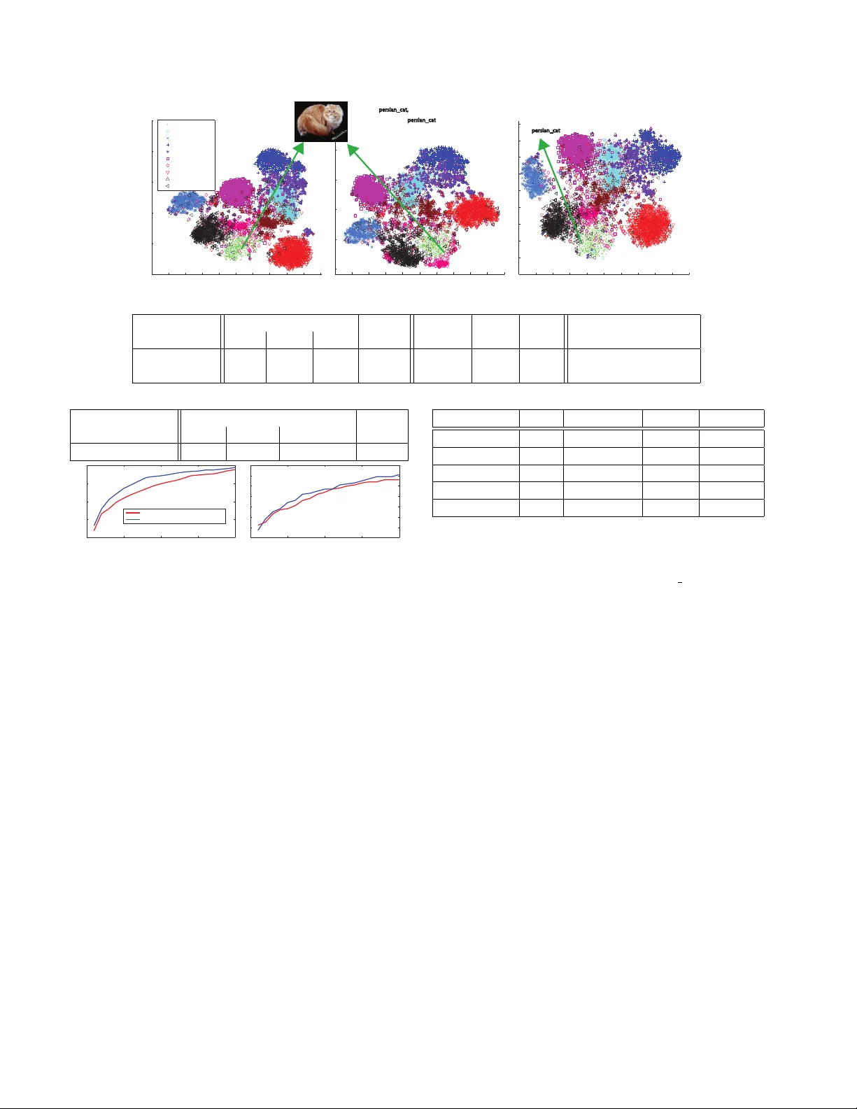
Semi-supervised V ocab ulary-inf ormed Lear ning Y anwei Fu and Leonid Sigal Disney Research y.fu@qmul.ac.uk, lsigal@disneyresearch.com Abstract Despite significant pr o gr ess in object cate gorization, in r ecent years, a number of important c hallenges r emain; mainly , ability to learn fr om limited labeled data and ability to r ecognize object classes within lar ge, potentially open, set of labels. Zer o-shot learning is one way of addressing these challenges, but it has only been shown to work with limited sized class vocabularies and typically r equires sep- aration between supervised and unsupervised classes, al- lowing former to inform the latter but not vice versa. W e pr opose the notion of semi-supervised vocab ulary-informed learning to alleviate the above mentioned challenges and addr ess pr oblems of supervised, zer o-shot and open set r ecognition using a unified frame work. Specifically , we pr o- pose a maximum mar gin framework for semantic manifold- based r ecognition that incorpor ates distance constraints fr om (both supervised and unsupervised) vocab ulary atoms, ensuring that labeled samples ar e pr ojected closest to their corr ect pr ototypes, in the embedding space, than to others. W e show that r esulting model shows impr ovements in super- vised, zer o-shot, and lar ge open set reco gnition, with up to 310K class vocabulary on A wA and ImageNet datasets. 1. Introduction Object recognition, and more specifically object catego- rization, has seen unprecedented advances in recent years with dev elopment of conv olutional neural networks (CNNs) [23]. Howe ver , most successful recognition models, to date, are formulated as supervised learning problems, in many cases requiring hundreds, if not thousands, labeled in- stances to learn a giv en concept class [10]. This exuberant need for lar ge labeled datasets has limited recognition mod- els to domains with 100’ s to few 1000’ s of classes. Humans, on the other hand, are able to distinguish beyond 30 , 000 ba- sic le vel cate gories [5]. What is more impressiv e, is the f act that humans can learn from few examples, by effecti vely lev eraging information from other object category classes, and even recognize objects without e ver seeing them ( e.g ., by reading about them on the Internet). This ability has spawned research in fe w-shot and zero-shot learning. Figure 1. Illustration of the semantic embeddings learned (left) using support vector regression ( SVR ) and (right) using the pro- posed semi-supervised vocabulary-informed ( SS-V oc ) approach. In both cases, t-SNE visualization is used to illustrate samples from 4 source/auxiliary classes (denoted by × ) and 2 target/zero- shot classed (denoted by ◦ ) from the ImageNet dataset. Decision boundaries, illustrated by dashed lines, are drawn by hand for vi- sualization. Note, that (i) large margin constraints in SS-V oc, both among the source/target classes and the external vocab ulary atoms (denoted by arrows and words), and (ii) fine-tuning of the seman- tic w ord space, lead to a better embedding with more compact and separated classes ( e.g ., see truc k and car or unicycle and tricycle ). Zero-shot learning (ZSL) has now been widely stud- ied in a variety of research areas including neural decod- ing by fMRI images [31], character recognition [26], face verification [24], object recognition [25], and video un- derstanding [17, 45]. T ypically , zero-shot learning ap- proaches aim to recognize instances from the unseen or unknown testing tar get categories by transferring informa- tion, through intermediate-le vel semantic representations, from known observed sour ce (or auxiliary) categories for which many labeled instances exist. In other words, super- vised classes/instances, are used as context for recognition of classes that contain no visual instances at training time, but that can be put in some correspondence with supervised classes/instances. As such, a general experimental setting of ZSL is that the classes in target and source (auxiliary) dataset are disjoint and typically the learning is done on the source dataset and then information is transferred to the tar- get dataset, with performance measured on the latter . This setting has a few important drawbacks: (1) it as- sumes that target classes cannot be mis-classified as source classes and vice versa; this greatly and unrealistically sim- plifies the problem; (2) the tar get label set is often relativ ely small, between ten [25] and several thousand unknown la- bels [14], compared to at least 30 , 000 entry level categories that humans can distinguish; (3) large amounts of data in the source (auxiliary) classes are required, which is problematic as it has been sho wn that most object classes hav e only few instances (long-tailed distribution of objects in the world [40]); and (4) the v ast open set vocab ulary from semantic knowledge, defined as part of ZSL [31], is not leveraged in any way to inform the learning or source class recognition. A few works recently looked at resolving (1) through class-incremental learning [38, 39] which is designed to dis- tinguish between seen (source) and unseen (target) classes at the testing time and apply an appropriate model – super- vised for the former and ZSL for the latter . Howe ver , (2)– (4) remain largely unresolved. In particular , while (2) and (3) are artifacts of the ZSL setting, (4) is more fundamen- tal. F or example, consider learning about a car by looking at image instances in Fig.1. Not knowing that other mo- tor vehicles exist in the world, one may be tempted to call anything that has 4-wheels a car . As a result the zero-shot class truck may ha ve large overlap with the car class (see Fig.1 [SVR]). Howe ver , imagine knowing that there also exist many other motor vehicles (trucks, mini-v ans, etc ). Even without ha ving visually seen such objects, the very basic kno wledge that they exist in the world and are closely related to a car should, in principal, alter the criterion for recognizing instance as a car (making the recognition cri- terion stricter in this case). Encoding this in our [SS-V oc] model results in better separation among classes. T o tackle the limitations of ZSL and towards the goal of generic open set recognition, we propose the idea of semi- supervised vocabulary-informed learning . Specifically , as- suming we have few labeled training instances and a large open set vocab ulary/semantic dictionary (along with textual sources from which statistical semantic relations among vo- cabulary atoms can be learned), the task of semi-supervised vocab ulary-informed learning is to learn a model that uti- lizes semantic dictionary to help train better classifiers for observed (source) classes and unobserv ed (target) classes in supervised, zero-shot and open set image recognition set- tings. Different from standard semi-supervised learning, we do not assume unlabeled data is av ailable, to help train clas- sifier , and only vocab ulary ov er the target classes is kno wn. Contributions: Our main contribution is to propose a novel paradigm for potentially open set image recognition: semi- supervised vocabulary-informed learning ( SS-V oc ), which is capable of utilizing vocabulary over unsupervised items, during training, to improve recognition. A unified maxi- mum margin frame work is used to encode this idea in prac- tice. Particularly , classification is done through nearest- neighbor distance to class prototypes in the semantic em- bedding space, and we encode a set of constraints ensur- ing that labeled images project into semantic space such that they end up closer to the correct class prototypes than to incorrect ones (whether those prototypes are part of the source or target classes). W e show that word embedding (word2vec) can be used effecti vely to initialize the se- mantic space. Experimentally , we illustrate that through this paradigm: we can achieve competitive supervised (on source classes) and ZSL (on target classes) performance, as well as open set image recognition performance with large number of unobserved vocab ulary entities (up to 300 , 000 ); effecti ve learning with fe w samples is also illustrated. 2. Related W ork One-shot Learning: While most of machine learning- based object recognition algorithms require large amount of training data, one-shot learning [12] aims to learn ob- ject classifiers from one, or only few e xamples. T o com- pensate for the lack of training instances and enable one- shot learning, knowledge much be transferred from other sources, for example, by sharing features [3], semantic at- tributes [17, 25, 34, 35], or conte xtual information [41]. Howe ver , none of pre vious works had used the open set v o- cabulary to help learn the object classifiers. Zero-shot Learning: ZSL aims to recognize nov el classes with no training instance by transferring knowledge from source classes. ZSL w as first e xplored with use of attrib ute- based semantic representations [11, 15, 17, 18, 24, 32]. This required pre-defined attribute vector prototypes for each class, which is costly for a large-scale dataset. Recently , semantic word vectors were proposed as a way to embed any class name without human annotation effort; they can therefore serv e as an alternative semantic representation [2, 14, 19, 30] for ZSL. Semantic word vectors are learned from large-scale te xt corpus by language models, such as word2vec [29], or GloV ec [33]. Ho wever , most of previ- ous w ork only use w ord vectors as semantic representations in ZSL setting, but have neither (1) utilized semantic word vectors explicitly for learning better classifiers; nor (2) for extending ZSL setting towards open set image recognition. A notable exception is [30] which aims to recognize 21K zero-shot classes gi ven a modest vocab ulary of 1K source classes; we explore vocab ularies that are up to an order of the magnitude larger – 310K. Open-set Recognition: The term “open set recognition” was initially defined in [37, 38] and formalized in [4, 36] which mainly aims at identifying whether an image belongs to a seen or unseen classes. It is also known as class- incremental learning. Howe ver , none of them can further identify classes for unseen instances. An exception is [30] which augments zero-shot (unseen) class labels with source (seen) labels in some of their experimental settings. Simi- larly , we define the open set image reco gnition as the prob- lems of recognizing the class name of an image from a po- tentially very large open set vocab ulary (including, but not limited to source and target labels). Note that methods like [37, 38] are orthogonal but potentially useful here – it is still worth identifying seen or unseen instances to be rec- ognized with different label sets as sho wn in experiments. Conceptually similar, but different in formulation and task, open-vocab ulary object retriev al [20] focused on retrieving objects using natural language open-vocab ulary queries. V isual-semantic Embedding: Mapping between visual features and semantic entities has been e xplored in two ways: (1) directly learning the embedding by regressing from visual features to the semantic space using Support V ector Re gressors (SVR) [11, 25] or neural network [39]; (2) projecting visual features and semantic entities into a common new space, such as SJE [2], WSABIE [44], ALE [1], DeV iSE [14], and CCA [16, 18]. In contrast, our model trains a better visual-semantic embedding from only few training instances with the help of large amount of open set vocab ulary items (using a maximum margin strategy). Our formulation is inspired by the unified semantic embedding model of [21], howe ver , unlike [21], our formulation is built on word v ector representation, contains a data term, and in- corporates constraints to unlabeled vocab ulary prototypes. 3. V ocabulary-inf ormed Learning Assume a labeled source dataset D s = { x i , z i } N s i =1 of N s samples, where x i ∈ R p is the image feature representation of image i and z i ∈ W s is a class label taken from a set of English words or phrases W ; consequently , |W s | is the number of source classes. Further , suppose another set of class labels for target classes W t , such that W s ∩ W t = ∅ , for which no labeled samples are av ailable. W e note that potentially |W t | >> |W s | . Given a new test image feature vector x ∗ the goal is then to learn a function z ∗ = f ( x ∗ ) , using all a vailable information, that predicts a class label z ∗ . Note that the form of the problem changes drastically depending on which label set assumed for z ∗ : Supervised learning: z ∗ ∈ W s ; Zero-shot learning: z ∗ ∈ W t ; Open set recognition: z ∗ ∈ {W s , W t } or, more generally , z ∗ ∈ W . W e posit that a single unified f ( x ∗ ) can be learned for all three cases. W e formalize the definition of semi-supervised vocab ulary-informed learning (SS-V oc) as follows: Definition 3.1. Semi-supervised V ocabulary-informed Learning (SS-V oc): is a learning setting that makes use of complete v ocabulary data ( W ) during training. Unlike a more traditional ZSL that typically makes use of the vocab ulary ( e.g ., semantic embedding) at test time, SS-V oc utilizes exactly the same data during training. Notably , SS-V oc requires no additional annotations or semantic knowledge; it simply shifts the burden from testing to training, lev eraging the vocabulary to learn a better model. The vocab ulary W can come from a semantic embedding space learned by word2vec [29] or GloV ec [33] on large- scale corpus; each vocab ulary entity w ∈ W is represented as a distributed semantic vector u ∈ R d . Semantics of em- bedding space help with kno wledge transfer among classes, and allow ZSL and open set image recognition. Note that such semantic embedding spaces are equi valent to the “se- mantic knowledge base” for ZSL defined in [31] and hence make it appropriate to use SS-V oc in ZSL setting. Assuming we can learn a mapping g : R p → R d , from image features to this semantic space, recognition can be carried out using simple nearest neighbor distance, e.g ., f ( x ∗ ) = car if g ( x ∗ ) is closer to u car than to any other word vector; u j in this context can be interpreted as the prototype of the class j . Thus the core question is then ho w to learn the mapping g ( x ) and what form of inference is optimal in the semantic space. For learning we propose dis- criminativ e maximum margin criterion that ensures that la- beled samples x i project closer to their corresponding class prototypes u z i than to any other prototype u i in the open set vocab ulary i ∈ W \ z i . 3.1. Learning Embedding Our maximum margin vocab ulary-informed embedding learns the mapping g ( x ) : R p → R d , from lo w-level features x to the semantic word space by utilizing maxi- mum margin strategy . Specifically , consider g ( x ) = W T x , where 1 W ⊆ R p × d . Ideally we want to estimate W such that u z i = W T x i for all labeled instances in D s (we would obviously want this to hold for instances belonging to unob- served classes as well, b ut we cannot enforce this explicitly in the optimization as we have no labeled samples for them). Data T erm: The easiest way to enforce the above objective is to minimize Euclidian distance between sample projec- tions and appropriate prototypes in the embedding space 2 : D ( x i , u z i ) = k W T x i − u z i k 2 2 . (1) W e need to minimize this term with respect to each instance ( x i , u z i ) , where z i is the class label of instance x i in D s . T o prev ent overfitting, we further re gularize the solution: L ( x i , u z i ) = D ( x i , u z i ) + λ k W k 2 F , (2) where k · k F indicates the Frobenius Norm. Solution to the Eq.(2) can be obtained through ridge regression. 1 Generalizing to a kernel version is straightforw ard, see [43]. 2 Eq.(1) is also called data embedding [21] / compatibility function [2]. Nev ertheless, to make the embedding more comparable to support vector regression (SVR), we employ the maximal margin strategy –  − insensiti ve smooth SVR (  − SSVR) [27] to replace the least square term in Eq.(2). That is, L ( x i , u z i ) = L  ( x i , u z i ) + λ k W k 2 F , (3) where L  ( x i , u z i ) = 1 T | ξ | 2  ; λ is regularization coef- ficient. ( | ξ |  ) j = max n 0 , | W T ?j x i − ( u z i ) j | −  o , | ξ |  ∈ R d , and () j indicates the j -th value of corresponding vector . W ?j is the j -th column of W . The con ventional  − SVR is formulated as a constrained minimization problem, i.e ., con vex quadratic programming problem, while  − SSVR employs quadratic smoothing [47] to make Eq.(3) differ - entiable e verywhere, and thus  − SSVR can be solv ed as an unconstrained minimization problem directly 3 . Pairwise T erm: Data term abov e only ensures that labelled samples project close to their correct prototypes. Howe ver , since it is doing so for many samples and over a number of classes, it is unlikely that all the data constraints can be sat- isfied exactly . Specifically , consider the following case, if u z i is in the part of the semantic space where no other enti- ties live ( i.e ., distance from u z i to any other prototype in the embedding space is large), then projecting x i further away from u z i is asymptomatic, i.e ., will not result in misclassifi- cation. Ho wever , if the u z i is close to other prototypes then minor error in regression may result in misclassification. T o embed this intuition into our learning, we enforce more discriminati ve constraints in the learned semantic em- bedding space. Specifically , the distance of D ( x i , u z i ) should not only be as close as possible, but should also be smaller than the distance D ( x i , u a ) , ∀ a 6 = z i . Formally , we define the vocab ulary pairwise maximal margin term 4 : M V ( x i , u z i ) = 1 2 A V X a =1  C + 1 2 D ( x i , u z i ) − 1 2 D ( x i , u a )  2 + (4) where a ∈ W t is selected from the open vocabulary; C is the margin gap constant. Here, [ · ] 2 + indicates the quadrat- ically smooth hinge loss [47] which is conv ex and has the gradient at e very point. T o speedup computation, we use the closest A V target prototypes to each source/auxiliary prototype u z i in the semantic space. W e also define similar constraints for the source prototype pairs: M S ( x i , u z i ) = 1 2 B S X b =1  C + 1 2 D ( x i , u z i ) − 1 2 D ( x i , u b )  2 + (5) 3 W e found Eq.(2) and Eq.(3) have similar results, on average, but for- mulation in Eq.(3) is more stable and has lower v ariance. 4 Crammer and Singer loss [42, 8] is the upper bound of Eq (4) and (5) which we use to tolerate variants of u z i (e.g. ’pigs’ Vs. ’pig’ in Fig. 2) and thus are better for our tasks. where b ∈ W s is selected from source/auxiliary dataset vocab ulary . This term enforces that D ( x i , u z i ) should be smaller than the distance D ( x i , u b ) , ∀ b 6 = z i . T o facil- itate the computation, we similarly use closest B S proto- types that are closest to each prototype u z i in the source classes. Our complete pairwise maximum margin term is: M ( x i , u z i ) = M V ( x i , u z i ) + M S ( x i , u z i ) . (6) W e note that the form of rank hinge loss in Eq.(4) and Eq.(5) is similar to DeV iSE [14], but DeV iSE only considers loss with respect to source/auxiliary data and prototypes. V ocabulary-informed Embedding: The complete com- bined objectiv e can now be written as: W = argmin W n T X i =1 ( α L  ( x i , u y i ) + (1 − α ) M ( x i , u z i )) + λ k W k 2 F , (7) where α ∈ [0 , 1] is ratio coef ficient of tw o terms. One prac- tical advantage is that the objective function in Eq.(7) is an unconstrained minimization problem which is differentiable and can be solved with L-BFGS. W is initialized with all zeros and con verges in 10 − 20 iterations. Fine-tuning W ord V ector Space: Above formulation works well assuming semantic space is well laid out and linear mapping is suf ficient. Howe ver , we posit that word vector space itself is not necessarily optimal for visual dis- crimination. Consider the following case: two visually sim- ilar categories may appear far away in the semantic space. In such a case, it w ould be dif ficult to learn a linear mapping that matches instances with category prototypes properly . Inspired by this intuition, which has also been expressed in natural language models [6], we propose to fine-tune the word vector representation for better visual discriminability . One can potentially fine-tune the representation by opti- mizing u i directly , in an alternating optimization ( e .g ., as in [21]). Howe ver , this is only possible for source/auxiliary class prototypes and would break re gularities in the se- mantic space, reducing ability to transfer kno wledge from source/auxilary to target classes. Alternati vely , we propose optimizing a global warping, V , on the word vector space: { W , V } = argmin W,V n T X i =1 ( α L  ( x i , u y i V ) + (1 − α ) M ( x i , u z i V )) + λ k W k 2 F + µ k V k 2 F , (8) where µ is regularization coefficient. Eq.(8) can still be solved using L-BFGS and V is initialized using an identity matrix. The algorithm first updates W and then V ; typically the step of updating V can conv erge within 10 iterations and the corresponding class prototypes used for final classifica- tion are updated to be u z i V . 3.2. Maximum Margin Embedding Recognition Once embedding model is learned, recognition in the se- mantic space can be done in a variety of ways. W e explore a simple alternativ e to classify the testing instance x ? , z ∗ = argmin i k W T x ∗ − φ ( u i , V , W, x ∗ ) k 2 2 . (9) Nearest Neighbor (NN) classifier directly measures the dis- tance between predicted semantic vectors with the proto- types in semantic space, i.e ., φ ( u i , V , W, x ∗ ) = u i V . W e further employ the k-nearest neighbors (KNN) of testing in- stances to average the predictions, i.e ., φ ( · ) is averaging the KNN instances of predicted semantic vectors. 5 4. Experiments Datasets . W e conduct our experiments on Animals with At- tributes (A wA) dataset, and ImageNet 2012 / 2010 dataset. A wA consists of 50 classes of animals ( 30 , 475 images in total). In [25] standard split into 40 source/auxiliary classes ( |W s | = 40 ) and 10 target/test classes ( |W t | = 10 ) is introduced. W e follow this split for supervised and zero- shot learning. W e use OverFeat features (downloaded from [19]) on A wA to make the results more easily compara- ble to state-of-the-art. ImageNet 2012 / 2010 dataset is a large-scale dataset. W e use 1000 ( |W s | = 1000 ) classes of ILSVRC 2012 as the source/auxiliary classes and 360 ( |W t | = 360 ) classes of ILSVRC 2010 that are not used in ILSVRC 2012 as target data. W e use pre-trained VGG- 19 model [7] to extract deep features for ImageNet. On both dataset, we use fe w instances from source dataset to mimic human performance of learning from few examples and ability to generalize. Recognition tasks . W e consider three different settings in a variety of e xperiments (in each experiment we carefully denote which setting is used): S U P E RV I S E D recognition, where learning is on source classes and we assume test instances come from same classes with W s as recognition vocab ulary; Z E R O - S H O T recognition, where learning is on source classes and we assume test instances coming from tar- get dataset with W t as recognition vocab ulary; O P E N - S E T recognition, where we use entirely open vocab- ulary with |W | ≈ 310 K and use test images from both source and target splits. Competitors . W e compare the following models, 5 This strategy is known as Rocchio algorithm in information retrieval. Rocchio algorithm is a method for relev ance feedback by using more rel- ev ant instances to update the query instances for better recall and possibly precision in vector space (Chap 14 in [28]). It was first suggested for use on ZSL in [17]; more sophisticated algorithms [16, 34] are also possible. SVM: SVM classifier trained directly on the training in- stances of source data, without the use of semantic em- bedding. This is the standard ( S U P E RV I S E D ) learning setting and the learned classifier can only predict the labels in testing data of source classes. SVR-Map: SVR is used to learn W and the recognition is done in the resulting semantic manifold. This corre- sponds to only using Eq.(3) to learn W . DeV ise, ConSE, AMP: T o compare with state-of-the-art large-scale zero-shot learning approaches we imple- ment DeV iSE [14] and ConSE [30] 6 . ConSE uses a multi-class logistic regression classifier for predict- ing class probabilities of source instances; and the pa- rameter T (number of top-T nearest embeddings for a giv en instance) was selected from { 1 , 10 , 100 , 1000 } that gives the best results. ConSE method in super- vised setting works the same as SVR. W e use the AMP code provided on the author webpage [19]. SS-V oc: W e test three different v ariants of our method. closed is a variant of our maximum margin leaning of W with the vocab ulary-informed constraints only from known classes ( i.e ., closed set W s ). W corresponds to our full model with maximum mar - gin constraints coming from both W s and W t (or W ). W e compute W using Eq.(7), but without optimizing V . full further fine-tunes the word vector space by also optimizing V using Eq.(8). Open set vocab ulary . W e use google word2v ec to learn the open set vocabulary set from a lar ge text corpus of around 7 billion w ords: UMBC W ebBase ( 3 billion words), the latest W ikipedia articles ( 3 billion words) and other web docu- ments ( 1 billion words). Some rare (low frequency) words and high frequency stopping words were pruned in the v o- cabulary set: we remove words with the frequency < 300 or > 10 mil lion times. The result is a vocab ulary of around 310K words/phrases with openness ≈ 1 , which is defined as openness = 1 − p (2 × |W s | ) / ( |W | ) . [38]. Computational and parameters selection and scalability . All experiments are repeated 10 times, to av oid noise due to small training set size, and we report an av erage across all runs. For all the experiments, the mean accuracy is reported, i.e ., the mean of the diagonal of the confusion matrix on the prediction of testing data. W e fix the parameters µ and λ as 0 . 01 and α = 0 . 6 in our experiments when only fe w training instances are a vailable for A wA (5 instances per class) and ImageNet (3 instances per class). V arying values of λ , µ and α leads to < 1% variances on A wA and < 0 . 2% v ariances on ImageNet dataset; but the experimental conclusions still hold. Cross-validation is conducted when 6 Code for [14] and [30] is not publicly av ailable. T esting Classes SS-V oc Aux T arg. T otal V ocab Chance SVM SVR closed W full S U P E RV I S E D X 40 40 2 . 5 52 . 1 51 . 4 / 57 . 1 52 . 9 / 58 . 2 53 . 6 / 58 . 6 53 . 9 / 59 . 1 Z E RO - S H O T X 10 10 10 - 52 . 1 / 58 . 0 58 . 6 / 60 . 3 59 . 5 / 68 . 4 61 . 1 / 68 . 9 T able 1. Classification accuracy ( % ) on A wA dataset for S U P E RV I S E D and Z E R O - S H OT settings for 100/1000-dim word2vec representation. more training instances are a vailable. A V and B S are set to 5 to balance computational cost and efficiency of pairwise constraints. T o solv e Eq.(8) at a scale, one can use Stochastic Gra- dient Descent (SGD) which makes great progress initially , but often is slow when approaches a solution. In contrast, the L-BFGS method mentioned abov e can achieve steady con vergence at the cost of computing the full objective and gradient at each iteration. L-BFGS can usually achie ve bet- ter results than SGD with good initialization, howe ver , is computationally expensi ve. T o le verage benefits of both of these methods, we utilize a hybrid method to solv e Eq.(8) in large-scale datasets: the solver is initialized with few in- stances to approximate the gradients using SGD first, then gradually more instances are used and switch to L-BFGS is made with iterations. This solver is moti vated by Fried- lander et al . [13], who theoretically analyzed and prov ed the conv ergence for the hybrid optimization methods. In practice, we use L-BFGS and the Hybrid algorithms for A wA and ImageNet respectiv ely . The hybrid algorithm can sav e between 20 ∼ 50% training time as compared with L-BFGS. 4.1. Experimental results on A wA dataset W e report A wA experimental results in T ab. 1, which uses 100/1000-dimensional word2vec representation ( i.e ., d = 100 / 1000 ). W e highlight the following observ a- tions: (1) SS-V oc variants ha ve better classification accu- racy than SVM and SVR. This validates the effecti veness of our model. Particularly , the results of our SS-V oc:full are 1 . 8 / 2% and 9 / 10 . 9% higher than those of SVR/SVM on supervised and zero-shot recognition respectiv ely . Note that though the results of SVM/SVR are good for supervised recognition tasks (52.1 and 51.4/57.1 respectiv ely), we can further improve them, which we attribute to the more dis- criminativ e classification boundary informed by the vocab- ulary . (2) SS-V oc: W significantly , by up to 8 . 1% , impro ves zero-shot recognition results of SS-V oc:closed . This v al- idates the importance of information from open vocab u- lary . (3) SS-V oc benefits more from open set vocab ulary as compared to word vector space fine-tuneing. The results of supervised and zero-shot recognition of SS-V oc:full are 1 / 0 . 9% and 2 . 5 / 8 . 6% higher than those of SS-V oc:closed . Comparing to state-of-the-art on ZSL: W e compare our results with the state-of-the-art ZSL results on A wA dataset in T ab . 2. W e compare SS-V oc:full trained with all source instances, 800 (20 instances / class), and 200 instances (5 in- Methods S. Sp Features Acc. SS-V oc:full W C N N OverFeat 78 . 3 800 instances W C N N OverFeat 74 . 4 200 instances W C N N OverFeat 68 . 9 Akata et al. [2] A+W C N N GoogleLeNet 73 . 9 TMV -BLP [16] A+W C N N OverFeat 69 . 9 AMP (SR+SE) [19] A+W C N N OverFeat 66 . 0 D AP [25] A C N N VGG19 57 . 5 PST[34] A+W C N N OverFeat 54 . 1 D AP [25] A C N N OverFeat 53 . 2 DS [35] W/A C N N OverFeat 52 . 7 Jayaraman et al. [22] A lo w-lev el 48 . 7 Y u et al. [46] A lo w-lev el 48 . 3 IAP [25] A C N N OverFeat 44 . 5 HEX [9] A C N N DECAF 44 . 2 AHLE [1] A lo w-lev el 43 . 5 T able 2. Zero-shot comparison on A wA. W e compare the state-of-the-art ZSL results using dif ferent semantic spaces (S. Sp) including word vector (W) and attribute (A). 1000 dimension word2vec dictionary is used for SS-V oc. (Chance-lev el = 10% ). Different types of CNN and hand-crafted low-le vel feature are used by dif ferent methods. Except SS-V oc (200/800), all instances of source data ( 24295 images) are used for training. As a general reference, the classification accuracy on ImageNet: C N N DECAF < C N N OverFeat < C N N VGG19 < C N N GoogleLeNet . stances / class). Our model achie ves 78 . 3% accuracy , which is remarkably higher than all previous methods. This is par- ticularly impressi ve taking into account the fact that we use only a semantic space and no additional attribute represen- tations that many other competitor methods utilize. Fur- ther , our results with 800 training instances, a small frac- tion of the 24 , 295 instances used to train all other meth- ods, already outperform all other approaches. W e ar gue that much of our success and improvement comes from a more discriminativ e information obtained using an open set v o- cabulary and corresponding large margin constraints, rather than from the features, since our method improv ed 25 . 1% as compared with D AP [25] which uses the same Ov er- Feat features. Note, our SS-V oc:full result is 4 . 4% higher than the closest competitor [2]; this improvement is statis- tically significant. Comparing with our work, [2] did not only use more powerful visual features (GoogLeNet Vs. OverFeat), but also employed more semantic embeddings (attributes, GloV e 7 and W ordNet-derived similarity embed- dings as compared to our word2vec). 7 GloV e[33] can be taken as an improv ed version of word2v ec. Large-scale open set recognition: Here we focus on O P E N - S E T 310 K setting with the large vocab ulary of approx- imately 310K entities; as such the chance performance of the task is much much lower . In addition, to study the ef- fect of performance as a function of the open vocabulary set, we also conduct two additional experiments with dif- ferent label sets: (1) O P E N - S E T 1 K − N N : the 1000 labels from nearest neighbor set of ground-truth class prototypes are selected from the complete dictionary of 310K labels. This corresponds to an open set fine grained recognition; (2) O P E N - S E T 1 K − RN D : 1000 label names randomly sampled from 310K set. The results are shown in Fig. 2. Also note that we did not fine-tune the word v ector space ( i.e ., V is an Identity matrix) on O P E N - S E T 310 K setting since Eq (8) can optimize a better visual discriminability only on a relati ve small subset as compared with the 310K v ocabulary . While our O P E N - S E T variants do not assume that test data comes from either source/auxiliary domain or target domain, we split the two cases to mimic S U P E RV I S E D and Z E RO - S H OT scenarios for easier analysis. On S U P E RV I S E D -like setting, Fig. 2 (left), our accuracy is better than that of SVR-Map on all the three different label sets and at all hit rates. The better results are largely due to the better embedding matrix W learned by enforcing maximum margins between training class name and open set vocab ulary on source training data. On Z E RO S H O T -like setting, our method still has a no- table adv antage ov er that of SVR-Map method on T op- k ( k > 5 ) accuracy , again thanks to the better embedding W learned by Eq. (7). Ho wev er, we notice that our top-1 accuracy on Z E RO S H OT -like setting is lo wer than SVR- Map method. W e find that our method tends to label some instances from target data with their nearest classes from within source label set. For example, “humpback whale” from testing data is more lik ely to be labeled as “blue whale”. Ho wever , when considering T op- k ( k > 5 ) ac- curacy , our method still has advantages o ver baselines. 4.2. Experimental results on ImageNet dataset W e further validate our findings on lar ge-scale ImageNet 2012/2010 dataset; 1000-dimensional word2v ec represen- tation is used here since this dataset has lar ger number of classes than A wA. W e highlight that our results are still bet- ter than those of two baselines – SVR-Map and SVM on (S U P E RV I S E D ) and ( Z E RO - S H O T ) settings respectiv ely as shown in T ab. 3. The open set image recognition results are shown in Fig. 4. On both S U P E RV I S E D -like and Z E R O - S H O T -like settings, clearly our frame work still has advan- tages over the baseline which directly matches the nearest neighbors from the vocab ulary by using predicted semantic word vectors of each testing instance. W e note that S U P E RV I S E D SVM results ( 34 . 61% ) on Im- ageNet are lo wer than 63 . 30% reported in [7], despite us- T esting Classes A wA Dataset Aux. T arg. T otal V ocab O P E N - S E T 1 K − N N 40 / 10 1000 ? O P E N - S E T 1 K − RN D (left) (right) 40 / 10 1000 † O P E N - S E T 310 K 40 / 10 310 K 0 5 10 15 20 50 55 60 65 70 75 80 85 90 95 100 Accuracy (%) Hit@k 0 5 10 15 20 0 10 20 30 40 50 60 70 80 Hit@k Accuracy (%) SVR−Map(OPEN SET − 1K−NN) SVR−Map(OPEN SET − 1K−RND) SVR−Map (OPEN SET − 310K) SS-Voc:W (OPEN SET − 1K−NN) SS-Voc:W (OPEN SET − 1K−RND) SSoVoc:W (OPEN SET − 310K) Figure 2. Open set recognition r esults on A wA dataset: Openness= 0 . 9839 . Chance= 3 . 2 e − 4% . Ground truth label is ex- tended for its variants. For example, we count a correct label if a ’pig’ image is labeled as ’pigs’. ? , † :different 1000 label settings. ing the same features. This is because only fe w , 3 sam- ples per class, are used to train our models to mimic human performance of learning from fe w e xamples and illustrate ability of our model to learn with little data. Howe ver , our semi-supervised vocabulary-informed learning can impro ve the recognition accurac y on all settings. On open set im- age recognition, the performance has dropped from 37 . 12% (S U P E RV I S E D ) and 8 . 92% (Z E RO - S H O T ) to around 9% and 1% respectiv ely (Fig. 4). This drop is caused by the intrinsic difficulty of the open set image recognition task ( ≈ 300 × increase in vocabulary) on a large-scale dataset. Howe ver , our performance is still better than the SVR-Map baseline which in turn significantly better than the chance-lev el. W e also e valuated our model with lar ger number of train- ing instances ( > 3 per class). W e observe that for standard supervised learning setting, the improvements achie ved us- ing vocab ulary-informed learning tend to somewhat dimin- ish as the number of training instances substantially grows. W ith large number of training instances, the mapping be- tween lo w-level image features and semantic words, g ( x ) , becomes better behaved and ef fect of additional constraints, due to the open-vocab ulary , becomes less pronounced. Comparing to state-of-the-art on ZSL. W e compare our results to sev eral state-of-the-art large-scale zero-shot recognition models. Our results, SS-V oc:full , are better than those of ConSE, DeV iSE and AMP on both T -1 and T -5 metrics with a very significant margin (improvement ov er best competitor, ConSE, is 3.43 percentage points or nearly 62% with 3 , 000 training samples). Poor results of DeV iSE with 3 , 000 training instances are largely due to the inefficient learning of visual-semantic embedding matrix. AMP algorithm also relies on the embedding matrix from DeV iSE, which explains similar poor performance of AMP −20 0 20 40 60 80 100 −100 −80 −60 −40 −20 0 20 40 60 80 100 SVR-Map −120 −100 −80 −60 −40 −20 0 20 40 60 80 −100 −50 0 50 100 150 SS-Voc:full persian cat hippopotamus leopar d humpback whale seal chimpanzee rat giant panda pig raccoon −50 0 50 100 −100 −80 −60 −40 −20 0 20 40 60 80 100 SS-Voc: closed SS-Voc:full : persian_cat, siamese_cat , hamster , weasel, rabbit, monkey , zebra, owl, anthropomorphized , cat SS-Voc:closed: hamster, persian_cat , siamese_cat, rabbit, monkey , weasel, squirrel, anteater , ca t, stuffed_toy SVR-Map: hamster , squirrel, rabbit, raccoon, kitten, siamese_cat, stuffed_to y, persian_cat , ladybug, puppy Figure 3. t-SNE visualization of A wA 10 testing classes. Please refer to Supplementary material for larger figure. T esting Classes SS-V oc Aux T arg. T otal V ocab Chance SVM SVR closed W full S U P E RV I S E D X 1000 1000 0.1 33 . 8 25.6 34.2 36.3 37.1 Z E RO - S H O T X 360 360 0.278 - 4.1 8.0 8.2 8.9 T able 3. The classification accuracy ( % ) of ImageNet 2012 / 2010 dataset on SUPER VISED and ZER O-SHO T settings. T esting Classes ImageNet Data Aux. T arg. T otal V ocab O P E N - S E T 310 K (left) (right) 1000 / 360 310 K 0 5 10 15 20 5 10 15 20 25 Accuracy (%) Hit@k 0 5 10 15 20 0 1 2 3 4 5 6 7 Accuracy (%) Hit@k SVR−Map (OPEN SET − 310K) SS-Voc:W (OPEN SET − 310K) Figure 4. Open set recognition results on ImageNet 2012/2010 dataset: Openness= 0 . 9839 . Chance= 3 . 2 e − 4% . W e use the synsets of each class— a set of synonymous (word or prhase) terms as the ground truth names for each instance. with 3 , 000 training instances. In contrast, our SS-V oc:full can lev erage discriminative information from open v ocabu- lary and max-margin constraints, which helps improve per - formance. For DeV iSE with all ImageNet instances, we confirm the observation in [30] that results of ConSE are much better than those of DeV iSE. Our results are a further significant improv ed from ConSE. 4.3. Qualitative results of open set image recognition t-SNE visualization of A wA 10 tar get testing classes is shown in Fig. 3. W e compare our SS-V oc:full with SS- V oc:closed and SVR. W e note that (1) the distributions of 10 classes obtained using SS-V oc are more centered and more separable than those of SVR ( e.g ., rat , persian cat and pig ), due to the data and pairwise maximum margin terms that help impro ve the generalization of g ( x ) learned; (2) the distribution of dif ferent classes obtained using the full model SS-V oc:full are also more separable than those of SS-V oc:closed , e.g ., rat , persian cat and raccoon . This can be attributed to the addition of the open-vocab ulary- informed constraints during learning of g ( x ) , which further improv es generalization. For example, we sho w an open Methods S. Sp Feat. T -1 T -5 SS-V oc:full W C N N OverFeat 8.9/9.5 14.9/16.8 ConSE [30] W C N N OverFeat 5.5/7.8 13.1/15.5 DeV iSE [14] W C N N OverFeat 3.7/5.2 11.8/12.8 AMP [19] W C N N OverFeat 3.5/6.1 10.5/13.1 Chance – – 2 . 78 e - 3 – T able 4. ImageNet comparison to state-of-the-art on ZSL: W e compare the results of using 3 , 000 / all training instances for all methods; T -1 (top 1) and T -5 (top 5) classification in % is reported. set recognition example image of “persian cat”, which is wrongly classified as a “hamster” by SS-V oc:closed . Partial illustration of the embeddings learned for the Im- ageNet2012/2010 dataset are illustrated in Figure 1, where 4 source/auxiliary and 2 tar get/zero-shot classes are sho wn. Again better separation among classes is largely attributed to open-set max-margin constraints introduced in our SS- V oc:full model. Additional examples of miss-classified in- stances are av ailable in the supplemental material. 5. Conclusion and Future W ork This paper introduces the problem of semi-supervised vocab ulary-informed learning, by utilizing open set seman- tic vocabulary to help train better classifiers for observed and unobserved classes in supervised learning, ZSL and open set image recognition settings. W e formulate semi- supervised v ocabulary-informed learning in the maximum margin framework. Extensive experimental results illus- trate the ef ficacy of such learning paradigm. Strikingly , it achiev es competiti ve performance with only fe w training instances and is relati vely robust to large open set vocab- ulary of up to 310 , 000 class labels. W e rely on word2vec to transfer information between observed and unobserv ed classes. In future, other linguistic or visual semantic embeddings could be explored instead, or in combination, as part of v ocabulary-informed learning. References [1] Z. Akata, F . Perronnin, Z. Harchaoui, and C. Schmid. Label- embedding for attribute-based classification. In CVPR , 2013. [2] Z. Akata, S. Reed, D. W alter , H. Lee, and B. Schiele. Eval- uation of output embeddings for fine-grained image classifi- cation. In CVPR , 2015. [3] E. Bart and S. Ullman. Cross-generalization: learning novel classes from a single e xample by feature replacement. In CVPR , 2005. [4] A. Bendale and T . Boult. T o wards open world recognition. In CVPR , 2015. [5] I. Biederman. Recognition by components - a theory of hu- man image understanding. Psychological Re view , 1987. [6] S. R. Bowman, C. Potts, and C. D. Manning. Learning distributed word representations for natural logic reasoning. CoRR , abs/1410.4176, 2014. [7] K. Chatfield, K. Simonyan, A. V edaldi, and A. Zisserman. Return of the devil in the details: Delving deep into conv o- lutional nets. In BMVC , 2014. [8] K. Crammer and Y . Singer . On the algorithmic implemen- tation of multiclass kernel-based vector machines. JMLR , 2001. [9] J. Deng, N. Ding, Y . Jia, A. Frome, K. Murphy , S. Bengio, Y . Li, H. Ne ven, and H. Adam. Large-scale object classifica- tion using label relation graphs. In ECCV , 2014. [10] J. Deng, W . Dong, R. Socher, L.-J. Li, K. Li, and L. Fei- Fei. Imagenet: A lar ge-scale hierarchical image database. In CVPR , 2009. [11] A. Farhadi, I. Endres, D. Hoiem, and D. Forsyth. Describing objects by their attributes. In CVPR , 2009. [12] L. Fei-Fei, R. Fergus, and P . Perona. One-shot learning of object categories. IEEE TP AMI , 2006. [13] M. P . Friedlander and M. Schmidt. Hybrid deterministic- stochastic methods for data fitting. SIAM J. Scientific Com- puting , 2012. [14] A. Frome, G. S. Corrado, J. Shlens, S. Bengio, J. Dean, M. Ranzato, and T . Mikolov . DeV iSE: A deep visual- semantic embedding model. In NIPS , 2013. [15] Y . Fu, T . Hospedales, T . Xiang, and S. Gong. Attribute learn- ing for understanding unstructured social activity . In ECCV , 2012. [16] Y . Fu, T . M. Hospedales, T . Xiang, Z. Fu, and S. Gong. T ransductive multi-vie w embedding for zero-shot recogni- tion and annotation. In ECCV , 2014. [17] Y . Fu, T . M. Hospedales, T . Xiang, and S. Gong. Learning multi-modal latent attributes. IEEE TP AMI , 2013. [18] Y . Fu, T . M. Hospedales, T . Xiang, and S. Gong. T ransduc- tiv e multi-view zero-shot learning. IEEE TP AMI , 2015. [19] Z. Fu, T . Xiang, E. Kodiro v , and S. Gong. zero-shot object recognition by semantic manifold distance. In CVPR , 2015. [20] S. Guadarrama, E. Rodner, K. Saenko, N. Zhang, R. Farrell, J. Donahue, and T . Darrell. Open-vocabulary object retrie val. In Robotics Science and Systems (RSS) , 2014. [21] S. J. Hwang and L. Sigal. A unified semantic embedding: relating taxonomies and attributes. In NIPS , 2014. [22] D. Jayaraman and K. Grauman. Zero shot recognition with unreliable attributes. In NIPS , 2014. [23] A. Krizhevsk y , I. Sutske ver , and G. E. Hinton. Imagenet classification with deep con volutional neural networks. In NIPS , 2012. [24] N. Kumar , A. C. Berg, P . N. Belhumeur, and S. K. Nayar . Attribute and simile classifiers for face verification. In ICCV , 2009. [25] C. H. Lampert, H. Nickisch, and S. Harmeling. Attribute- based classification for zero-shot visual object categoriza- tion. IEEE TP AMI , 2013. [26] H. Larochelle, D. Erhan, and Y . Bengio. Zero-data learning of new tasks. In AAAI , 2008. [27] Y .-J. Lee, W .-F . Hsieh, and C.-M. Huang.  -SSVR: A smooth support vector machine for  -insensitive regression. IEEE TKDE , 2005. [28] C. D. Manning, P . Raghav an, and H. Schutze. Intr oduction to Information Retrie val . Cambridge Uni versity Press, 2009. [29] T . Mikolov , I. Sutskev er , K. Chen, G. Corrado, and J. Dean. Distributed representations of words and phrases and their compositionality . In Neural Information Pr ocessing Systems , 2013. [30] M. Norouzi, T . Mikolov , S. Bengio, Y . Singer , J. Shlens, A. Frome, G. S. Corrado, and J. Dean. Zero-shot learning by con vex combination of semantic embeddings. ICLR , 2014. [31] M. Palatucci, G. Hinton, D. Pomerleau, and T . M. Mitchell. Zero-shot learning with semantic output codes. In NIPS , 2009. [32] D. Parikh and K. Grauman. Relative attributes. In ICCV , 2011. [33] J. Pennington, R. Socher , and C. D. Manning. Glove: Global vectors for word representation. In EMNLP , 2014. [34] M. Rohrbach, S. Ebert, and B. Schiele. Transfer learning in a transductiv e setting. In NIPS , 2013. [35] M. Rohrbach, M. Stark, G. Szarvas, I. Gurevych, and B. Schiele. What helps where – and why? semantic relat- edness for knowledge transfer . In CVPR , 2010. [36] H. Sattar , S. Muller , M. Fritz, and A. Bulling. Prediction of search targets from fixations in open-w orld settings. In CVPR , 2015. [37] W . J. Scheirer , L. P . Jain, and T . E. Boult. Probability models for open set recognition. IEEE TP AMI , 2014. [38] W . J. Scheirer, A. Rocha, A. Sapkota, and T . E. Boult. T o- wards open set recognition. IEEE TP AMI , 2013. [39] R. Socher , M. Ganjoo, H. Sridhar, O. Bastani, C. D. Man- ning, and A. Y . Ng. Zero-shot learning through cross-modal transfer . In NIPS , 2013. [40] A. T orralba, R. Fergus, and W . Freeman. 80 million tin y images: A large data set for nonparametric object and scene recognition. IEEE TP AMI , 2008. [41] A. T orralba, K. P . Murphy , and W . T . Freeman. Using the forest to see the trees: Exploiting context for visual object detection and localization. Commun. ACM , 2010. [42] I. Tsochantaridis, T . Joachims, T . Hofmann, and Y . Altun. Large margin methods for structured and interdependent out- put variables. JMLR , 2005. [43] A. V edaldi and A. Zisserman. Efficient additiv e kernels via explicit feature maps. In IEEE TP AMI , 2011. [44] J. W eston, S. Bengio, and N. Usunier . Wsabie: Scaling up to large v ocabulary image annotation. In IJCAI , 2011. [45] Z. W u, Y . Fu, Y .-G. Jiang, and L. Sigal. Harnessing object and scene semantics for large-scale video understanding. In CVPR , 2016. [46] F . X. Y u, L. Cao, R. S. Feris, J. R. Smith, and S.-F . Chang. Designing category-le vel attributes for discriminative visual recognition. CVPR , 2013. [47] T . Zhang. Solving large scale linear prediction problems us- ing stochastic gradient descent algorithms. In ICML , 2004.