Developing an ICU scoring system with interaction terms using a genetic algorithm

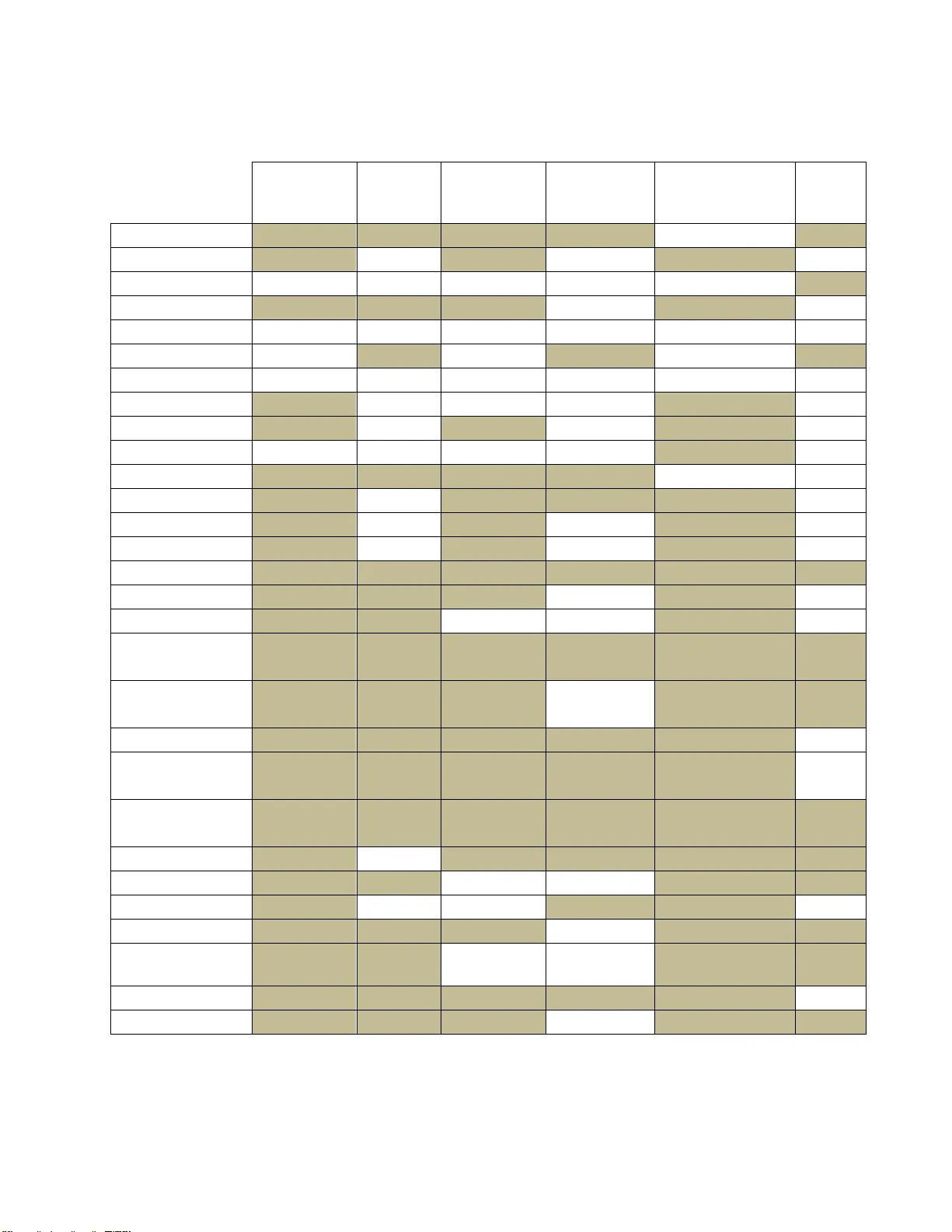
1 Developing an ICU scoring system with interaction terms using a genetic algorithm  ,  Chee Chun, Gan a ,*  , Gerard P. , Learmont h b a Department of Systems and Information En gineering, Un iversity of V irginia, Charlottes ville, VA, USA b Frank Batten School of Leader ship and Public Policy Abstract ICU mort ality scoring systems attempt to predict patient mortality using predict ive models with various clinical p redictors. Examples of such systems are APACHE, SAPS and MPM. However, most such scoring systems do not actively look for and include interaction terms, despite physicians intuitively taking su ch interactions into account when making a diagnosis. One barrier to including such terms in predictive m odels is the difficulty of using most variable selection methods in high-dimensional datasets. A genetic algorithm framework for variable selection with logistic regression models is used to search for two-way interaction terms in a clinical dataset of adult ICU patients , with separate models being b uilt for each cat egory of diagnosis u pon admittance to t he ICU . The mo dels h ad good discrimination acr oss all categories, with a weighted average AUC of 0.84 (>0.90 for several categories) and the genetic algorithm was able to f ind several significant interaction terms, which may be able to pro vide greater insight into mortality pred iction for health practitioners. Th e GA selected models had improved performance against stepwise selection and random forest models, and provides greater flexibility in terms of variable select ion by being able to optim ize over any modeler- defined mo del performance metric instead of a specific variable importance metric.  Conflicts of interest : We have no competin g interests.  Role of the funding source: We received no fund ing for this study.  Corresponding auth or: Department of Systems and Information E ngineering, Univ ersity of Virginia, 151 Engineer’s Way, P .O. Box 400747, Charlottesville, VA 22 904, Tel.: 434 -924-5393 E-mail address : cg 8pa@virginia.edu (Chee Chun Gan) 2 Keywords: ICU scorin g system, predictive modelling, genetic algorithm, variable selection, interaction terms 1 Introduction Pr edictive modelling in healthcare is a rapidly growing field . Recent innovations in information systems use in hospitals has resulted in a massive increase in the availability and accuracy of patient electronic health records (EHRs) and other sources of med ical data. This Data Science boom has enabled the developm ent of more predictive analytics tools to aid health practitioners in tasks such as d iagnosing illnesses, assessing the likelihood of p atient readmission, and predicting patient mortality. Many predict ive scoring systems for adult ICU patient mortality have been developed. Among the mo st popular are the Acute Ph ysiology and Chronic Health Evaluation (APACHE) score, the Mortality Probability M odels (MPM) and the Simplified Acute Physiology Score (SAPS ). Most of these predictive models are built using physiological, clinical or therapeutic variables that are routinely collected in the ICU, either as a first day sn apshot or dynamically updated throughout a patient’s ICU stay. Furthermore, mo st such scori ng systems are based on a form of logistic regression to predict a patient’s probability of mortali ty. The Acute Physiology And Chro nic Health Evaluation (APACHE) score was developed by Knaus et. al. [1] to assess the severity of illness of crit ically ill adult patients admitted to the intensive care u nit (ICU). The first APACHE model consisted of 34 physiologic predictors selected using expert judgement. Further refinements to the APACHE mod el have followed with APACHE II, III and IV. APACHE II has been wi dely used in many hospitals and healthcare f acilities for benchmarking purposes [2]. The APACHE II score is b ased on several clinical and ph ysiologic measurements taken when a patient is first admitted to th e ICU [3]. For APACHE II, the score is calculate d from the following 13 predictors: age, alveolar-arterial gradient (A- aO 2 ) or partial pressure art erial oxygen (PaO 2 ) depending on the fraction of inspired oxygen (FiO 2 ), rectal t emperature, mean arterial pressure (MAP), arterial pH, heart rate, respiratory rate, sodium (serum), potassium (serum), creatinine, 3 hematocrit, white b lood cell count and Glasgow Coma Scale score. The predictor values are used in a univariate logistic regression model to predict mortality. APACHE III expanded on APACHE II by including five additional physiologic predictors to the APS component, and included t hree two -way interaction terms as well [4]. The latest version, APACHE IV, uses a multivariate logistic regression model with a much larger dat aset (110,588 pat ients) compared to it s predecessors [5]. However, the exact variables and methodology used in APACHE IV have not been published. The Simplified Acute Physiology Score (SAPS) was originally based on the APS p redictors included in APACHE [6]. Expert judgement was used to reduce the number of predictors to 13 physiologic variables and patient age. SAPS II later included 4 additional demographic variables, bringing the to tal up t o 17 (12 physiologic, 5 demo graphic) [ 7]. The predictor val ues w ere assigned a score by binning over the range of values (similar t o APACHE), with the sum of these scores then being used in a logistic regression for patient mortality. The Mortality Probability Model (MPM) scoring system was developed using 12 variables in a multivariate logistic regression model [8]. Initially b ased only on data at the time of admission, further studies incorporated data taken 24 hours and 48 hours aft er admission. MPM II was later d eveloped which included models built f or data at ad mission, after 24 hours, after 48 hours and after 72 hours [9]. Two -way interaction terms were considered in MPM II, but were eventually re jected for not satisfying the author’s criteria for inclusion. The aforementioned ICU scoring systems h ave been validated with good performance in numerous studies [10]. However, a common point among these scoring systems is that they are mainly developed using p redictors selected by subje ct matter expert judgement and mostly do not include interaction terms (APACHE III and possibly APACHE IV are exceptions). However, intuitively when pred icting patient mortality it is likely t hat the existence of certain conditions in conjunction may p ose a much gr eater health risk than when these condit ions exist independently. Many physicians would naturally take i nto account the interplay of all physiologic variables when making a d iagnosis, instead of considering ea ch variable independently. In a complex problem such as predicting mortality, there may be many 4 interaction effects that can give a dditional power to the model. In many cases, health practitioners are aware of such effects based on their experience and judgement b ut have no way of quantifying the strength of the interactions due t o the lack of re search into the inclusion of interaction terms. Thus, for the sake of model parsimon y interaction terms are often omitted (e.g. the MPM II model rejected interaction t erms if there was n o “clinical plausibility” behind them [9]). However, it is also p ossible t hat ben eficial interaction effects exist which are currently unknown to health practitioners and therefore would not be included in a model designed mainly using expert knowledge. Thus, this exploratory study aims to develop a prototype ICU morta lity scoring system using machine learning methods (a genetic algorithm) f or variable selection instead of re lying solely on expert knowledge. By evaluating the efficacy of models with interaction t erms included, we aim to explore the potential benefits of using a variab le selection method t hat can handle a large number of interactions t o develop such models and hopefully find novel interactions that may not be well-known to health practitioners. 2 ICU m ortality dataset For this study, we obtained a datase t of 224,418 patient records with 12 binary comorbid ities, 5 categorical clinical predictors, and 2 numeric predictors 1 . A similar dataset was used to evaluate APACHE IV against APACHE III [5]. Table 2. 1 b elow summarizes the list of predictors included in the dataset. Table 2.1: Predictors in ICU dataset Binary predictors Categorical predictors Numeric predictors operative, emergency, aids, myeloma, lymphoma, cirrhosis, tumorwm, immunosup, hepfail, copd, diabetic, dialysis visit priorloc gender ethnic dx_group age APS 1 Private communication with Dr. Andrew Kra mer, formerly of th e Cerner Corporation. 5 The first t wo binary predictors represent whether a patient is in the ICU for an operative or emergency procedure. The remaining binary predictors represent the absence or presence (0 or 1 respectively) of the listed comorbidities in the patient upon being admitted to t he ICU. For the numeric predict ors, “age” lists the pat ient’s age i n years (integer) while the Acute Physiology Score (APS) is an integer score b ased on a regression model using 12 clinical predictors, some of which are included in the list of APACHE II predictors. The first categorical predictor, “visit”, indicates how many t imes the patient has been admitted to th e ICU and ranges from 1 to 9. “Priorloc” indicates t he patient’s location prior to entering the ICU, e.g. home, other hosp ital IC U etc. “Gender” and “ethnic” indicate the sex and ethnicity (6 levels) of the pat ient respectively. “Dx_group” stores the p atient’s diagnosis code, which is given by a physician upon admittance to t he ICU. The diagnosis code is assigned b ased on the physic ian’s diagnosis of the patient’s condition. The diagnosis code is a factor (with 122 levels in this dataset) which can be grouped into 16 categories. Note that a p atient being admitted to the ICU can exhibit multiple condit ions, e.g. head trauma and interc erebral hemorrhage. However, only a sin gle primary condition (as judged by the attendin g physician) is recorded in the data. Thus, each patient can only be associated with a single “dx_grou p” value. While the ICU d ataset was closely related to the data us ed to develop the AP ACHE models, several key variables were omitted (Glasgow Coma Scale, AaDO2/PaO2, pH arterial, potassium). Thus, we were unable t o calculat e the APACHE II score (or any of the other commonly u sed ICU scoring systems) for the patients in the dataset as a baseline comparison. 3 Data preproce ssing The d ataset in cluded two binary predictands, “icudead” and “hosdead”. These labels represent whether the patient passed away in the ICU or subsequently in the hospital after being discharged from the ICU. For the purposes of this study, we only considered patient mortality in the ICU as there could be multiple complicating factors involved in hospital mortality that are not captured in the d ataset. Thu s, all p atients who p assed away in the hospital were removed, 6 leaving only patients that survived or passed away in t he ICU. Records that contain missing data in the categorical/binar y predictors were remo ved, while records with missing data in the numeric predictors w ere replaced by the mea n. As a result, the final da taset used for the analysis consisted of 154,281 patient records. Several issues arose d uring the initial an alysis of the dataset. First ly, the APS predictor is an aggregate measure of several clinical predictors. Th us, it provides a general indication of the patient’s health condit ion b ut does n ot provide information on t he factors contributing to the score. Wh ile it performed adequately as an input to the original APACHE f ormulation, in order to explore potential interaction terms (especially with comorbidities) it would be more meaningful to expand the APS into its constituent components. Doing so add ed 12 additional numeric predictors to the dataset. These nu meric predictors, together with t he age of the patient, were scaled t o have mean 0 and variance 1 in order t o reduce the effects of multi - co llinearity. Secondly, the “visit” variable was changed from a 9 level factor to a 2 level factor indicating whether th e patient was a first t ime visitor to the ICU, or a re peat visitor. Repeated visits to the ICU could be indicative of additional health c omplications or a poo r h ealth cond ition in general, leading to high er risk of mortality. However, the vast majority of pat ients h ad “visit” levels of either 1 or 2 (>98%), with a small minority having more than 2 visit s. As such, we could combine all “visit ” levels 2 or greater into a single level, grea tly reducing the complexity of the model while retaining most of the predictive power. Lastly, the “dx_group” predictor with 122 levels resu lted in a very sparse matrix with many diagnosis codes belonging to very few patients, or none at all. In addition, consultations with subject matter experts (physicians at t he University of V irginia Hospital ICU) revealed that in many cases the initial d iagnosis is subjective and th e diagnosis code assigned to the patien t can vary substantially from p hysician to ph ysician. Thus, the existing data on diagnosis cod es is likely to be fairly noisy. However, there is less cont ention regarding the category of diagnosis. For example, it may be unclear whether a patient is suffer ing from b acterial pneumonia or viral pneumonia, but most physicians would ca tegorize the diagn osis as a respiratory condition. 7 Following this line of reasoning, th e various diagnosis codes were aggregated into the following 12 categories shown in Table 3. 1. Table 3.1: Diagnosis categories in ICU dataset Category # of patients Cardiovascular diagnosis 52,630 Cardiovascular surgery 9,690 Respiratory diagnosis 23,047 Respiratory surgery 3,478 Neurologic diagnosis 20,222 Neurologic surgery 6,510 Gastrointestinal diagnosis 11,422 Gastrointestinal surgery 8,975 Trauma diagnosis 6,869 Trauma surgery 2,261 Metabolic diagnosis 6,839 Genitourinary diagnosis 2,338 Total 154,281 Furthermore, our discussion with subject matter experts suggested that it would likely improve model performance to subset the d ata according to the categories shown above. A patient admitted to t he ICU for trauma injuries could have a very different set of mortality predictors than a patient admitted for respiratory p rob lems. Many of the original ICU scoring systems were intentionally designed for ease of use with pen and paper calculations, and d eveloping different models for different diagnosis codes would have greatly complicated the scoring process. However, with the widespread use of information technology in hospitals it should no longer be a requirement to be constrained to a single aggregated model for all patient conditions. B y developing a model for each diagnosis category, we ar e also able to better explore potential interaction t erms without the co nfounding effects of other con ditions. Appendix A lists the final predictors considered in the models . For each subset, logistic regression models were used to fit the d ata to pred ict ICU mortality. This choice was informed by several f actors. Firstly, logistic regression models are widely used and well-understood by p hysicians. Pr edictions from logistic regression mo dels are also easier 8 to calculate without special software and can be performed using spreadsheets or m ob ile apps, compared to models su ch as random fores ts or artificial neural networks. Secondly, many studies of ICU mortality have used logistic regression models with similar predictors and demonstrated good p erformance. One of th e primary concerns with lo gistic re gression models is the possible p resence of non-linear predictors, which are common in medicine due to the prevalence of homeostatic processes in living organisms. However, empirical results show that logistic regression models p erform well on many medical datasets even without first applying transformations to non-linear predictors. Lastly, logistic regression models are easily interpretable, especially with regard s to interaction t erms. Interaction terms are explicitly defined in logistic regress ion models and thus th eir effe cts can be more easily isolated and evaluated. After deciding on the model, we now have to determine the appropriate quantitative metric to use for model evaluation. As the GA provides great f lexibility in the choice of f itnes s function, there are many possib le options. The area und er the Receiver Operating Characteristic (ROC) curve is a metric th at is commonly u sed in machine learn ing for model comparison and has also seen widespread use and accep tance in t he medical communit y. The ROC curve is d erived by using the model’s predictions to plot the true positive rate (TPR) against the false p ositive rate (FPR) for various values of the decision threshold. The area under t he ROC curve (AUC) can therefore be u sed as a metric of a model’s d iscriminative power, with a larger AUC indicating that a model has a h igher probability of ran king a randomly chosen positive instance h igher than a randomly chosen negat ive instance. It should be noted that the AUC alon e should not be taken as a definitive measure of a model’s effectiveness. A model with a h igher AUC does not necessarily perform better than another model with a lower AUC, as the AUC represents the models’ performance across all possib le thresholds. When a model is u sed for classif icat ion a specific threshold has to be chosen in order for a class pred iction to b e made, and the relative performance of the models at that specific threshold could well differ f rom their AUC rankings. Nevertheless, we chose to use AUC as the model evalu a tion criteria as the AUC serves well as a general indicator of model performance and has been used extensi vely in evaluating APACHE, SAPS, MPM and other such scoring systems. 9 4 Using a genet ic algorithm for variable selection A genetic algorithm was developed to select potential main effect and interaction terms for the logistic regression model. The genetic algorithm consist s of a population of cand idate predictor sets , termed “chromosomes”, which are evaluated according to a user -specified fitness function at each generation of the algorithm. High performing chromosomes have a higher chance to pass on t o the next generation, with some modifications such as re combination with other high performing chromosomes or random mutation (performed according to a var ying probability p arameter). A maximum chromosome size is d efined to set an u pper bound for the maximum number of predictors included in the final solution obtained at the end of the specified number of generations. Appendix B describes the GA selection procedure in greater detail. For each diagnosis subset of the ICU dat aset, the GA framework was used to perform variable selection for a logistic regression model, using AUC as the fitness function. Each subset was split into ten folds for cross-validation u sing random sampling without replacement, with t he size of folds 1-9 being set to f loor(   ), where N is t he total numb er of records in the subset. Fold 10 contains the remaining records after folds 1-9 have been drawn. Each candidate solution consists of a set of predictors, which are then evaluated on each test fold in turn after b eing trained on t he remaining nine fold s, en suring that the test data never ove rlaps with the t raining data. The ten resulting AUC scores are then averaged to obtain the overal l AUC score for the aforementioned set of p redictors . Table 4.1 below sh ows the settings for the GA’s meta - parameters used for all subsets. Table 4.1: GA parameter settings Chromosome population size 30 Min/Max number of predictors 5/100 Maximum number of generations 250 Recombination probability 0.5 to 0.2 Mutation probability 0.01 to 0.2 10 For each diagnosis subset, 5 runs were p erformed using different initial random nu mber generator seeds, and the best performing GA result was chosen. The following section describes the results from each subset, as well as p rovides some comparisons with other modelling methods. 5 Results and discu ssion Due to the limitations of t he variables provided in the dataset, we were unable to compare the AUC of the GA selected model against other ICU scoring systems like APACHE, SAP S II and MPM II. To provide a comparison, for each subset we developed a logistic regression model u sing stepwise selection according to Akaike Informati on Criterion (AIC ) and a ran dom forest model with 500 tre es. The same ten f olds used for the GA selection p rocess were used to evaluate t he AUC with each of the stepwise selected logistic re gression models and random forest models. Table 5.1 below shows the mean AUCs obtained for the stepwise -selected logistic regression model, the random forest model, and the GA-selected logistic regression model resp ectively. For each sub set, the stand ardized mortality ratio (SMR) of t he GA -selected logistic regression models was not significantly d ifferent from 1.0, indicating no major differences b etween the observed number of deaths and the expected n umber of deaths. The Wilcoxon signed rank test was used to test for significance of the difference in AUCs between the GA vs stepwise selection and GA vs random forest by comp aring the paired AUC scores in each fol d us ed i n c ross - validation for the two selection methods evaluated. 11 Table 5.1: Mean AUC for logistic regression (stepwise), random forest and logistic regression (GA) Stepwise Random forest GA GA vs Step GA vs RF AUC AUC AUC p-vals* p-vals* Cardiovascular diagnosis 0.8187 0.8605 0.8300 0.0039 0.00 20 Cardiovascular surgery 0.8614 0.8684 0.8921 0.0137 0.08 40 Respiratory diagnosis 0.7719 0.7761 0.7852 0.00 20 0.1602 Respiratory surgery 0.8290 0.8213 0.9159 0.0098 0.0059 Neurologic diagnosis 0.7824 0.8390 0.8050 0.0137 0.00 20 Neurologic surgery 0.8833 0.8678 0.9200 0.00 20 0.00 20 Gastrointestinal diagnosis 0.8265 0.8383 0.8426 0.0039 0.4922 Gastrointestinal surgery 0.8199 0.8545 0.8692 0.0137 0.00 20 Trauma diagnosis 0.8170 0.8805 0.8597 0.0039 0.08 40 Trauma surgery 0.8383 0.8896 0.9065 0.0039 0.1934 Metabolic diagnosis 0.8560 0.8580 0.8952 0.00 20 0.0098 Genitourinary diagnosis 0.7844 0.7855 0.8599 0.00 20 0.0273 * p-values calculated by performing Wilcoxon signed-rank test on AUC scores for c ross- validation folds It can be seen that the discrimin ation of the GA -selected model is fairly goo d, ranging from 0.7852 to 0.9200 across t he various subsets. The GA -sele cted model significantly outperformed the stepwise select ed model in all 12 categories (at a 0.05 significance level), while the random forest model was better in 2 catego ries and worse in 5 categories. In particular, the GA-sele cted model performed markedly better than both stepwise selection and random forest in the “respiratory surgery” and “genitourinary diagnosis” categories. Tables 5 .2 and 5.3 below su mmarize the significant predictors in each category. Each column represents a diagnosis category, while t he rows represent the main effects t erms. A highlighted cell in a column indicates that t he main effect is included in the model for the indicated diagnosis category. The numbers in each cell indicate the variab les with which the term has significant pair- wise interactions. For example, in the model f or cardiovascular diagnosis t he “visit” t erm is a significant main effect with no interaction t erms, while the “age” term has significant interactions with “dialysis”, “temp”, “sodium” and “album”. 12 Table 5.2 : Model summary for diagnosis categories 1-6 Cardio diag Cardio surg Resp diag Resp surg Neuro diag Neuro surg 1 visit 4,20 20,28 26 2 ipriorloc 12,18 11,14 4,16,21 3 gender 23 4 age 16,18,25,28 1,26 11 2,22,24 5 op erative 6 emerg 29 19 7 aids 8 myeloma 25 12,23 9 lymphoma 10 cirrhosis 24 11 tumorwm 18 2,4,12 12 imm.sup 2 11 8,28 13 hepfail 26,27 28 25 14 copd 19,22 2,26 22 15 diabetic 22,27 16 21 25,27 22 16 dialysis 4,26 15,21,26 26 2 17 ethnic 18,25 24 19 18 temp 2,4,19,20,27 11,28 19 20 20,22,26,28 19,22, 29 19 map 20,21,22,25, 27 20 18,20,21,23, 26 17,21,28,29 6,18,23 20 hr 23 1,19,21 1,19 18,21 18 21 rr 25 29 19 15,20,22,25, 27 2,19,22,23,27 22 urine 27 23 4,14,18,21,23, 24, 25 15,18 23 wbc 26,28 29 22 8,21,22,24 3,19 24 hcrit 26 17 4,10,22,23 25 25 sodium 4,8,17,19 13,15,22 26 creat 13,16,23,24 4,16 14,16,19 18,27 1 27 gluc 13,15,18,19, 22 15,21,26,28 28 album 4,23 18 13,29 12,18,19,27 29 bili 6,21 23,28 18 13 Table 5.3 : Model summary for diagnosis categories 7- 12 Gastro diag Gastro surg Trauma diag Trauma surg Meta diag Genito diag 1 visit 15 24 2 ipriorloc 22,25 13 28 3 gender 18 18,23 26 28 22 4 age 22 22,25 19,21,27 11 5 op erative 6 emerg 22 7 aids 8 myeloma 9 lymphoma 10 cirrhosis 15 11 tumorwm 22 22,24,27 4 12 imm.sup 23 27 13 hepfail 28,29 2,23 14 copd 15,23 26,28 15 diabetic 1,26 14 10 16 dialysis 24,25,26 22 20 20 27,28,29 17 ethnic 18 18 temp 3,22,24 3,17,19,21,23 26 24,26 19 map 20 23 18,23,25 4,23,26 20,22,28 20 20 hr 19,23 16,21,25,27 16,25,29 19 19 21 rr 18,20,25,29 4,25 22,28 22 urine 2,4,11 16,18 4,11 6 19,27 3,21 23 wbc 12,20 13,19 3,14,18,19,28 19 25,26 24 hcrit 16 18 11 1,18 25 sodium 2,16,27 4,19,20,21 20,21 23 26 creat 15,16,29 3,14,18,19 18,23 27 gluc 25 11,20,29 4 22 12,16 28 album 13 2,23 14 3,19 16,21 29 bili 13,26 21,27 20 16 The current implementation of the GA does n ot directly select for model sparsity in t he fitness function, which results in the GA -selected models having a fairly large numb er of predictors. While a penalty for model size could b e added to the fitness funct ion, doing so comes with significant downsides. Firstly, such a p enalty function co uld interfere with the GA selection 14 process by forcing the GA to b ecome too greedy and prematurely weed out predictors that may initially provide little improvement to the A UC, but would improve t he fitness in the presence of certain other predictors. Secondly, the determination of the appropriate penalty function is non- trivial and has a significant effect on the GA’s p erformance. However, it should be noted that the larger size does not necessarily translate to a large r burden on data collect ion, as the majority of th e addit ional variab les are interaction terms der ived f rom the original 29 main effects variables which are already routinely collected. Furthermore, the GA -selected models can b e further refined using expert judgement or other variable selection methods, b oth of which become more viable once the number of potential predictors has been reduced using the GA. As expected, the models for each diagnosis category differ substantially. However, the patient’s age, numb er of visits and various APS predictors gen erally are sign ificant in almo st every category, which is con sistent with the findings of other ICU scoring systems. The presence of diabetes and whether the patient is on dialysis are also significant in several models, while the presence of AIDS, myeloma, cirrhosis, and whether the patient was admitted for operative purposes is relatively insignificant. Further examination of the models also re veals some inter esting observati ons. First ly, the “emergenc y” predictor is signific ant in most of the diagnosis categories pertaining to surgery. Secondly, mo st of the models include significant interactions amongst the APS predictors (together with significant APS main e ffects terms). These interaction effects h ave not been included in other ICU scorin g systems th at use the APS score as an aggregate predictor. Thirdly, the GA was ab le to identify several inter actions in the dataset that cou ld potentially be avenues f or fu rther study. For example, the ethn icity of the patient is sign ificant in several categories (cardiovascular d iagnosis, neurological diagnosis, trauma diagnosis) along with interactions with APS predictors such as sodium and t emperature. The gender of the p atient also has significant inter actions with APS pred ictors in various diagnosis categories. 15 6 Conclusions The results of the study show that ther e is potential benefit in utilizing machine learning methods, in this case a genetic algorithm for variable selection, in developing IC U scoring systems which include interaction terms. Using AUC as a measure of model performance, the GA -selected logistic regression models had comparable or better discrimination than stepwise - selected logistic regression models or random forest models. We also show that d eveloping different models for various diagnosis categories rat her than using a single model for all ICU patients may yield improved model performanc e as well as provide in sight in the form of significant interaction terms f or each particular diagnosis category. Thus, the GA selection process can serve as a useful first step in developing mod els to support physicians in predicting patient mortality. However, the GA-selection procedure also comes with some notabl e drawbacks. Th e first is the procedure run-time, which can be very signi ficant compared to other variable selection methods. On the other hand, t he GA selection procedure is ab le to deal with an arbitrarily large number of potential p redictors, unlike several common variable selection procedures. Furthermore, the long run -time is only applicable during model development (or upd ating) not during patient classification. Secondly, there is n o theoretical guarantee that th e GA will f ind globally optimum model s t hat generalize well. Th e models returned b y t he GA shou ld be validated on another dataset that should ideally cont ain the same pred ictors used in other ICU scoring systems, which would allow a better comparison of the models with interaction effects. Th e GA could also be coupled with other variable selection procedures to try to prune t he final number of predictors, which could make the models more generalizable to ot her datasets. 16 References [1] Knaus WA, Zimmerman JE, Wagner DP, Draper EA and Lawrence DE. APACHE acute physiology and chronic health evaluation: a physiologically based classification system. Crit Care Med 1981; 9 (8):591- 7. [2] Nouira S, Belghith M, Elatrous S, Jaafoura M, Ellouz i M , Boujdaria R, et al. Predictive value of severity scoring systems: comparison of four models in Tunisian adult intensive care units. Crit Care Med 1998; 26 (5):852-9 [3] Knaus WA, Draper EA, Wagner DP and Zimmerman. APACHE II: A severity of disease classification system. Crit Care Med 1985; 13 :818- 830. [ 4] Knaus WA, Wagner DP, Draper EA, et al. The APACHE III pro gnostic system. Risk prediction of hospital mortality for critically ill hospitali zed adults. Chest 1991; 100:1619. [5] Zimmerman JE, Kramer AA, McNair DS, Malila FM. Acute Physiology and Ch roni c Health Evaluation (APACHE) IV: h ospital mortality assessmen t f or t oday's critically ill patients. Crit Care Med 2006; 34:1297. [6] Le Gall JR, Loirat P, Alperovitch A, Glaser P, Pranthil C, M athieu D et al.. A simplified acute physiology score for ICU patients. Crit Care Med 1984; 12 :975-977. [7] Le Gall JR, Lemeshow S and Saulnier F. A new Simplified Acute Physiology Score (SAPS II) based on a European/North American multicenter study. JAMA1993; 270 (24):2957-2963. [8] Lemeshow S, Teres D , Pastides H, Avrunin JS an d Steingrub JS. A method for p redicting survival and mortality of ICU patients using objectively derived weights. Crit Care M ed 1985; 13 (7):519- 525. [9] Lemeshow S, Tere s D, Klar J, Avrunin JS, Gehlbach SH and Rapopo rt J. M ortality Probability Models (MPM II) based on an international cohort of intensive care unit patients. JAMA 1993; 270 (20):2478-2486 [10] Kuzniewicz M W, Vasilevskis EE, Lane R, et al. Variation in ICU risk -adjusted mortality: impact of methods of assessment and potential confounders. Chest 2008; 133:1319. 17 Appendix A: List of predic tors and de scriptions Name Description Type visit # of times patient has been admitted to ICU Factor (1- 9) ipriorloc Prior location of patient Factor (emergen cy department, other floor, home, ICU transfer, other hospital, other h ospital ICU, other, SDU, telemetry) gender Male or female Factor (0 = Male, 1 = Female) age Patient age in year s Numeric operative Procedure is op erative Binary emerg Procedure is emerg ency Binary aids Presence of Acquir ed Immune Deficiency Syndro me (AIDS) Binary myeloma Presence of m yeloma (cancer of plasma cells) Binary lymphoma Presence of ly mphoma (can cer of lymphatic syste m) Binary cirrhosis Presence of cirrh osis Binary tumorwm Presence of tum or with metastasis Binary immunosup Presence of im munosuppressive disorder Binary hepfail Presence of hepatic fail ure Binary copd Presence of chronic obstructive pulmonary diseas e Binary diabetic Presence ofdiabet es Binary dialysis Patient is on dialysi s Binary ethnic Ethnicity of patient Factor (other unkn own, African American, Asian, Cauca sian, Hispanic, Native Am erican) temp Temperature Numeric map Mean arterial pr essure Numeric hr Heart rate Numeric rr Respiratory rate Numeric urine Urine output Numeric wbc White blood cell c ount Numeric hcrit Hematocrit Numeric sodium Sodium level Numeric creat Creatinine level Numeric gluc Glucose level Numeric album Albumin level Numeric bili Bilirubin level Numeric 18 Appendix B: Geneti c algorithm modification for inclu ding interacti on terms in high-dimensi onal datasets The biggest challenge in the in clusion of interaction t erms in variable selection problems is the dramatic increase in the solut ion space. For now, we constrain ou rselves to only considering second order interaction terms, i.e. only pair -wise interactions. For n main effects terms, this adds     second order interaction ter ms. For relatively small n the additional terms can st ill be handled using the traditional GA variable selection chromosome (a single vector of 0 -1 bits of length n+     to indicate all possible variables), but this implementation quickly becomes unwieldy. For 100 variables an addit ional 4,950 interaction terms are added, and for 200 variables this jumps to 19,900. Thus for problems with hundreds o f va riables a new chromosome formulation is needed. In order to solve t he scalability issue, we propose some modifications to the original chromosome formu lation. While only seco nd order interaction t erms are examined here, the basic technique for ex tending the GA framework remains applicable for hig her order interactions at the cost of greatly increased computation time. Firstly, a maximum chromosome length l is defined. This all ows the modeler to specify an upper bound for model sparsity, as in many instances modelers may not be interested in creating a model with thousands of variables. Se condly, instead of ea ch bit in the chromosome simply being 0 -1 to indicate the absence or p resence of a variable, each b it now stores the index number of a variable to be included, and 0 if t he bit is a “dummy b it”. Dummy bits are placeholder b its within the chromosome that reserve space f or a potential variable t o enter the model. This f ormulat ion allows for chromosomes representing models with a differing number of included variables while still allowing chromosome length to be hom ogenous within the population, which simplifies the crossover operation. Figure B.1: Chromosome with dummy bits 19 The chromosome in Figure B.1 shows a chromosome of length 6 with 3 d ummy bits, with variables 1,5 and 26 included in th e model. Each new chromosome is initialized with dummy bits in all positions, and the number of initial variables is chosen uniformly betw een 1 and L (maximum number of variab les). Pr e-seeded variables can also be utilized instead of random selection. The i ndex positions of these variables are also chosen by sampling without replacement f rom the available L positions, after which the variabl es (either randomly chosen or pre-seeded) are then filled into their respective index positions o n the chromosome. After determining the fitness levels of all members of the population, a selection procedure is then use d to choose several parent c hromosome s. One common sele ction metho d is tournament selection, where several candidates are chosen randomly to participate in a “tournament” during which th e fitness values of competing chromosomes are compared, with the winn er being selected as a parent c hromosome. Th is parallels the biological process of natural selection where mo re fit individuals in a p opulation have a greater chance of reproducing and p assing on their genes to their offspring. In our implementation, the chromosome with the maximum fi t ness is automatically passed on to the next generatio n (elitist selection to preserve the best found solution), along with a mutation of the chromosome with the maximum fitness. The remaining members of the population are chosen by tournament selection, with each tournament containing 10 randomly selected candidates. Once parent chromosomes have been selected, the crossover operation is used to generate offspring, or child chromosomes. Again, there are various forms of crossover operators used with the underlying notion of combining the gen es from mu ltiple (usually two ) parent chromosomes into a single offspring. The most basic crossover operator is a fixed point crossover, with the crossover point usually being the midpoint of the chromosome. The underlying notion behind the crossover operator is that a high -performing parent chromosome should contain certain elements that contribute to its fitness score. In the case of a variable selection p roblem, it could be that high p erforming chromo somes contain a larger ratio of th e “correct” variables. By comb ining the chromosom es of two parents, the crossover operator attempts t o generate children which also have a high likelihood of equal or improve d 20 performance. The crossover operator can be applied according to a predefined probabilistic parameter setting. For example, a crossover probability of 0.5 would indicate that a pair of parents wou ld have their chromosomes combined h alf the time. The other half of the time would s ee both paren ts bein g passed on t o the next generatio n without mixing their chromosomes, similar to elitist selection. The current chromosome formulation can handle an arbitrary number of main effects terms in addition to interaction terms as long as the modeler specifies a maximum number of variables. As the chromosome length is homogenou s, the aforementioned sin gle point crossover operator can be ap plied on the modified chromosome, with some additional checks to ensure that duplicate variables are removed. The mutation operator is separated into two t ypes, a d eletion mutation and an add ition mutation. The del etion mutation replaces a random n on-dummy bit with a value of 0, con verting it to a dummy bit and re moving the selected variable from the model. Th e addit ion mutation replaces a random d ummy bit with a randomly selected variable that is currently not includ ed in the model. Both types of mutat ion occur independently with probabilities P a and P d specified by the modeler. Both mutations occur simultaneously with probability P a *P d , resulting in one variable being sw itched out for another. Both crossover and mutation (addit ion and deletion) are applied with a variable probability across the GA’s run time. A minimum and maximum probability is defined for ea ch operator (the same parameters apply t o both types of mutation). The p robabilities for each operator are adjusted each generation so as to vary from minimum t o maximum or vice versa. The crossover probability p c is initialized to p c_max = 0.5 at generation 0, and t hen varies across each generation i according t o Equa tion 1 below u ntil finally reaching p c_min = 0.2 after maxgen iterations.   󰇛  󰇜        󰇡   󰇢         (1) The mutation prob ability p m (for both addition and deletion) is initialized t o p m_min = 0.01 and varies linearly throughout the run until it reaches p m_max = 0.2 after maxgen iterations, as shown in Equation 2. 21   󰇛  󰇜      󰇡   󰇢        (2) These varying p robabilities are chosen to obtain a higher chance of crossover with less mutation at the beginning of the GA run (increased exploration of solution space), an d a lower chance of crossover with more mutat ions at the en d of the run (increased exploitation of good solutions in population). In addit ion, the GA framework ensures the model ob eys strong h ierarchy. Each time an interaction term enters the model th rough either re combination or the addition mutation, a check has to be performed to ensure that the corresponding main effects terms are also included. If not , the missing main effects terms are inserted into random d ummy bit p osit ions. If a main effect term is deleted through the deletion mutation, then all interaction terms that include the aforementioned main effect term are also dele ted. Lastly, in order to prevent selection of models that over -fit the data, all fitness fun ctions are evaluated u sing 10-fold cross-validation. The data is partitioned into ten folds, with the models being successively tested on a single fold and trained on the other nine folds. The final fitness is then obtained by averaging the model fitness o ver all ten test folds. With this pro cess, there is never any ove rlap between data used f or training models, and data used for evaluating the fitness.