Dynamic matrix factorization with social influence

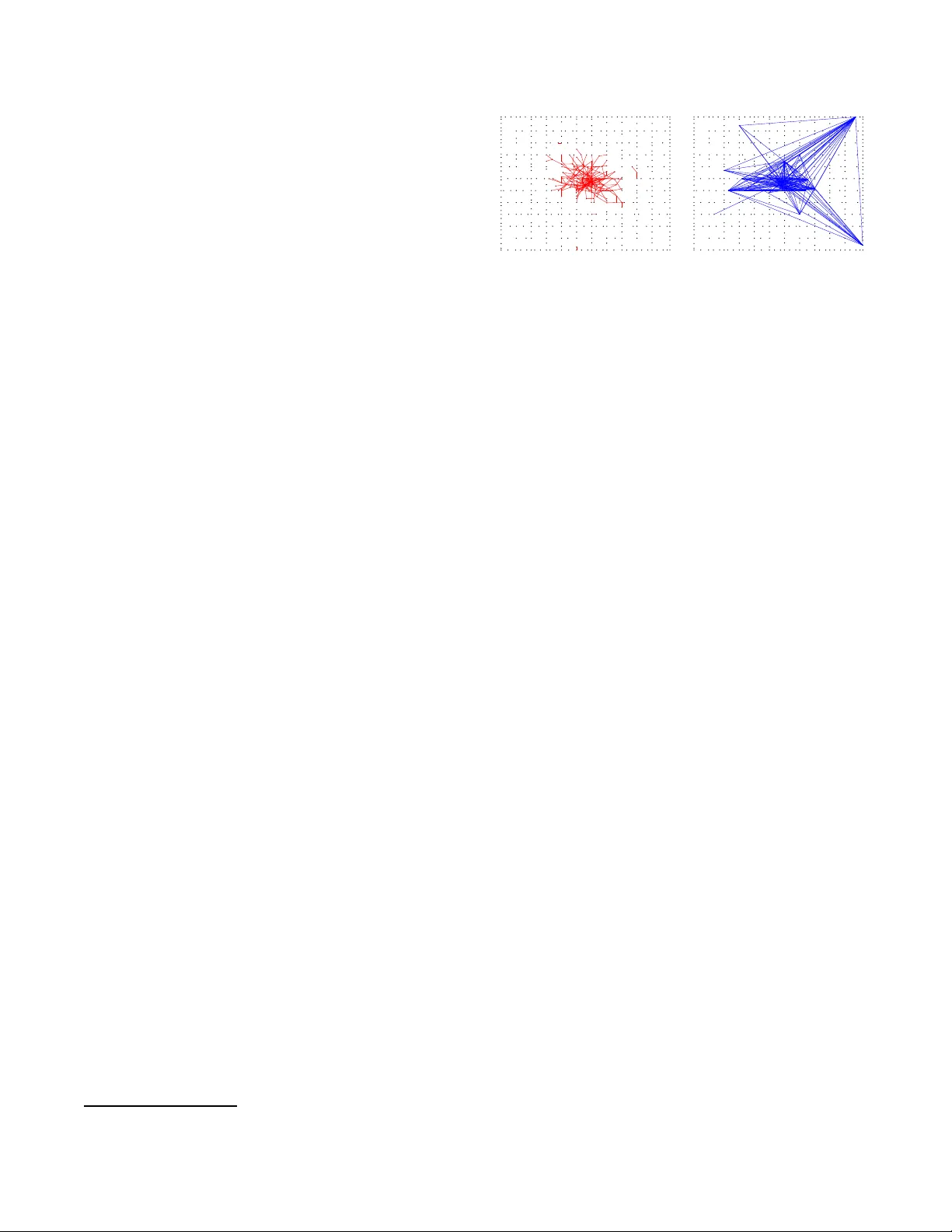
2016 IEEE INTERN A TIONAL WORKSHOP ON MA CHINE LEARNING FOR SIGN AL PR OCESSING, SEPT . 13–16, 2016, SALERNO, IT AL Y D YNAMIC MA TRIX F A CTORIZA TION WITH SOCIAL INFLUENCE Aleksandr Y . Aravkin Department of Applied Mathematics Univ ersity of W ashi ngton Seattle, W A 98195 USA K ush R. V arshne y , and Liu Y ang Mathematical Sciences Department IBM Thomas J. W atson R esearch Center Y orktown Heights, NY 10598 USA ABSTRA CT Matrix factorization is a key component of collaborati ve filtering- based recommendation systems because it allows us to complete sparse user-by-item ratings matrices under a l o w-rank assumption that encodes the belief that si milar users give similar ratings and that simi lar items garner simil ar r atings. This paradigm has had immeasurable practical success, but it is not the complete story for understanding and inferring t he preferences of people. First, peoples’ preferences and their observ able manifestations as ratings e volv e o ver time along general patterns of trajectories. Second , an indi vidual person’ s preferences e volve ov er time throug h influence of t heir so cial connection s. In this p aper , we de velop a unified pro- cess model for both types of dynamics within a state space approach, together with an ef ficient optimization scheme for estimation within that model. The model combines elements from recent de velop- ments in dynamic matrix factorization, opinion dynam ics and social learning, and trust-based recommendation. The estimation builds upon recent adv ances in numerical nonlinear optimization. Em- pirical results on a large-scale data set from t he Epinions website demonstrate consistent reduction in root mean squared error by consideration of the two types of dyn amics. Index T erms — S ocial network, dyna mic inference 1. INTRODUCTION In many applications, there is a population of learning problems, which we might suppo se share an un derlying distribution o r are oth- erwise correlated. In the collaborativ e filtering setting , for instance, each user h as a set of it ems he or she prefers and the fact that on e user prefers items A an d B increases our con fidence that users who prefer item A also tend to prefer item B. Simil ar typ es of related- ness also arise in social media conte xts. There are no w many large and highly-successful online co mmunities, where each user ca n be modeled as a learn ing problem (for instance , for selecting adv ertise- ments, search results, or restaurant recommendations), and there is significant benefit to be found i n t he correlations and patterns that extend a cross users. Howe ver , there is e very reason to suspect that the same conn ections between learning problems that allow better group models in the static case can also h elp in the dy namic setting as well. For instance, we might suppose that the drifting behaviors of the lea rning problems a re also correlated , and this correlation can be used to model the grou p’ s drift, before adjusting to each individu al member . This perspecti ve has led t o the e xtension of static matrix factorization-bas ed approaches for recommend ation t o incorpo- rate rich temporal models of t he change in preferences ov er time [1, 2, 3, 4 ]. In these appro aches, the rows of the data matrix repre- sent the users and columns t he items. Such appro aches use a state space model t o capture temporal dynamics, where the state is the set o f user factors, and typically use a restri ctiv e class of mod els to model dy namics (typically linear), and errors ( t ypically Gaussian ), to allo w for standard estimation techniques based on the Kalman filter . Scalability is an imp ortant issue i n all approaches, as both the state space and measurement space can be quite large. T wo contrib utions of this paper are (1) rel axing restrictions of pre vious work on dynamic matrix factorization by allo wing a wide v ariety of nonlinear and non -Gaussian state space models, and (2) sho wi ng ho w t o design tractable and scalable inference for large- scale problems. W e b uild on the optimization viewpoint on Kalman smoothing [5], stepping a way from the forw ard-backw ard recursion that is typically used and instead fo rmulating a single large optimiza- tion problem to be solv ed using quasi-Newton algorithms. The third contrib ution is to inc orporate dynamic pheno mena in user behavior: social influen ce , which is separate from the general group-le vel user rating trajectories captured in the temporal mo dels of [1, 2, 3, 4]. A person may eat at a restaurant with a menu tha t he or she does not much fanc y i f a group of friends has decide d to eat there. A legislator may vote for a bil l sponsored by a secon d legisla- tor if that second leg islator voted for a past bill sponsored by the first legislator . In general, a person’ s emotions, preferences, opinions, decisions, and actions are affected by other people. Social influence includes co nformity , compliance, and obed ience as v arious manifes- tations. Opinion dynamics and so cial learning are models for these types of ef fects as they e volv e over time [6, 7]. Social influence in recommendation via opinion dynamics has been considered in [8], but not within the matrix factorization paradigm. W e tackle the ch allenge of modeling social influence in a unified manner with dy namic matrix factorization by inc orporating a regu- larization term for the dynamics that can easily inco rporate known social influence structure via the g raph Laplacian. In particular , we assume that we are able to observe the e xistence of soc ial conn ec- tions among users as a graph at all times. Such data can be ex- tracted from websites such as Epinions in which use rs publicly de- clare which other users they trust. Give n the observed tempo rally- e volving social influence graph, we includ e a regularization term that imposes the belief deri ved from opinion d ynamics and social learn- ing theory tha t future preferences of a user should be similar to the preferences of users that he or she trusts. Mathematically , this is encoded using the Laplacian of the social influence graph . Such a term has been used previously in static, but not dynamic, settings to impo se similarity [9, 10]. W e are able to include this term into the overall formulation because of the flexibility afforded to us by the o ptimization vie wpoint on Kalman smo othing; it w ould no t hav e been able to be included otherwise. 978-1-509 0-0746-2/16 /$31.00 c  2016 IEEE Our use of t he trust graph to inform recommendation shares sim- ilarity with recen t papers su ch as [1 1, 12, 13, 14 ], b ut those formula- tions are for the static, not dyn amic, setting. Moreov er , the specific way in which the social in fluence graph affects the objectiv e is dif fer- ent than our formulation. The ev olution of the trust grap h over time is analyzed in [13], b ut the temporal insights are not used directly in the recommendation task. The fi nal co ntribution herein is an experimental study on real- world large-scale ratings data that sho ws how including both the general preference trajectory dynamics and the more individualized social influence dynamics to impro ve predictiv e accuracy . In partic- ular , we conduct the study on data from the Epinions website, the only ava ilable large, real-world data we kno w of con taining a time- v arying trust graph al ong with the more typical time-v arying user- item ratings matrix. W e sho w an impro vement in root mean squared error (RMSE) o f dynamic matrix factorization with social influence for a l arge range of choices of the rank parameter (n umber of f actors) in the matrix factorization . 2. BA CKGROUND In this sec tion, we revie w static factorization, and show ho w to ex- tend from static formulations to dynamic matrix fac torization. 2.1. Notation and Static Matrix F actorization Suppose we are interested in the p references of m users for n prod- ucts, where some users hav e expressed their preferences for some products, stored in t he vector z ∈ R p , with 1 ≤ p ≤ mn . Let R ∈ R m × n denote the full matrix listing all preferences; R is ob- served on ly through the dataset z : z = A ( R ) , where A is an operator from R m × n → R p . Factorized matrix formulations look for a lo w rank representa- tion R = U V T , where U ∈ R m × k , and V ∈ R n × k . The ap- proach requires the mod eler to select the latent dimension k , typi- cally k << min( m, n ) . The factorized representation allows a fast computation of A ( R ) . Note that R ij = h U i , V j i , an inner product between two vectors of length k . Therefore, A ( U V T ) can be computed in e xactly k p operations, which is a key point for tractable approaches in large-sc ale settings. Optimization fo rmulations to obtain factors U, V are of the form min U,V ρ  z − A ( U V T )  + φ 1 ( U ) + φ 2 ( V ) , (1) where ρ is a measu re of misfi t between observed and predicted data (often least squares), φ 1 and φ 2 are regularization penalties, and A ( U V T ) = A ( V ⊗ I )ve c( U ) , (2) with A ∈ R p × mn a sparse mask t hat selects the observed entries and vec the vectorization operator . Problem (1) is noncon vex, but has bee n t remendously successful in practice. Factorization-based approaches all o w matrix com pletion for ex tremely larg e-scale systems by a voiding costly SVD comp uta- tions [15, 16, 17, 18]. While we are interested in dyn amic settings, we use an approach analogous to (1) to initialize o ur (con ve x) dyna mic inference formu- lation. In the follo wi ng section, we detail the dynamic formulation, and then explain the initialization procedure we use prior to entering the dynamic phase. 2.2. Dynamic Matrix Facto rization Datasets t hat track product preferences h av e a longitudinal structure, as users continue to ev aluate products in time. W e are most inter- ested in dynamic settings where change s in user preferences can be modeled. The symmetry of U and V in (1) is therefore brok en; in- deed, we are much mo re interested in modeling and inference of user dynamics , so we focus on U . The general dynamic model is as follows. W e assume our dataset has a natural representation ov er N observation times, t 1 , . . . , t N . W e assume that U t is an unkno wn time series (total size m × k × N ) t o be determined, and define some process transi- tion matrix G t , a kno wn li near pr ocess that describes the tr ansition. The models V t can be estimated e.g. by solving (1) independently , or obtaining an av eraged model V over N time po ints. T reati ng U t as the unkno wn state an d V t as a known measure- ment model, we arriv e at the linear model U t +1 = G t U t + ǫ t , z t = A t  U t V T t  + ν t (3) where ǫ t describes process noise, and ν t ∈ R p t is observ ati on noise with kno wn covarian ce matrix S t . Note that dimensions of observ a- tion vectors z t can vary b etween time points, hence z t ∈ R p t . One of our main contributions is to define an appropriate model G t that can capture inertia, or smoothness, in user preferences, and combine i t with measurem ent information and so cial trust. Before we discuss the dynamic model, we re vie w ho w information about influence can be brought to bear on the inference problem. 2.3. Initialization Proc edure Inference over the dynamic mod el (3) is a con ve x problem in { U t } , as long as { V t } are assumed fixed . Howe ver , to obtain these mea- surement models V t , we need to initial ly factor each matrix R t into form U t V t . The key idea here is to e xtract V t , which then beco me part of the fixed measureme nt model, as we track U t . T o obtain the factorization R t ≈ U t V T t , we follow the app roach of [18], and solve the p roblem min U t ,V t 1 2  k U t k 2 F + k V t k 2 F  s . t . k b − A ( U t V T t ) k 2 ≤ σ. (4) using publicly availab le code. Formulation (4) controls the quality of fac torization by means of both the rank k of the factors, an d the regularizer 1 2  k U t k 2 F + k V t k 2 F  ; it is we ll known (see e.g. [16, 1 7]) that k R k ∗ = inf R = U V T 1 2  k U t k 2 F + k V t k 2 F  . Therefore, e very solution U t , V t corresponds to ˆ R t = U t V T t with k R t k ∗ ≤ 1 2  k U t k 2 F + k V t k 2 F  , where ( U , V ) minimize the Frobe- nius norm ov er the set { U t , V t : k b − A ( U t V T t ) k 2 ≤ σ } . Thus, e ven if the ran k k is p icked to be too large, the formulation (4) maintains control of mo del complexity through minimizing the func- tional. W e performed our ex periments over ranks k = 5 , 10 , 15 , 20 (see in Fi gures 2–5), and the static RMSE (obtained from the init ial factorization (4)) is slightly increasin g in k but do es not v ary much. 2.4. Similarity Usin g the Graph Laplacian Our main goal is t o incorporate the ef fect of social trust on chang es in preferences. In particular , su ppose that for each time p oint, we are gi ven matrices W t ∈ R m × m that en code the trust/influence b etween users. Reca ll that degree matrices corresponding to W t are giv en by diagonal D t ∈ R m × m , with d ii = P m i ′ =1 w ii ′ , while graph Laplacian matrices L t are defined by L t = D t − W t . W e want to look for solutions U t that are more consistent with relationships enc oded by L t , which mak es it more l ikely for pref- erences users with mutual trust to ev olve in a mutually consistent manner , i.e. along level sets of the follo wing functional: φ t ( U t ) = tr  U T t L t U t  . (5) The key missing detail is continuity in preferences; or some prior on the smoothness of preference chan ges over time. In the next sec- tion, we sho w ho w to i ncorporate this notion in order to track dy- namic preference systems of form (3). 3. PROPOSED FORMULA TION T o capture the smoothness or inertia of user preferences over time, we use a mo del common to phy sical systems. In particular , we posit the e xistence of a velocity state ˙ U , together with a simp le inte gration model to link U and ˙ U :  ˙ U U  t +1 =  I 0 dt I   ˙ U U  t + w , w ∼ N (0 , Q ) . (6) This model is frequently used for smoo th systems in dynamic infer - ence [5]. Pairs of elements ( ˙ U t ( i, j ) , U t ( i, j )) are pairwise corre- lated with kno wn covarian ce [19] Q =  dt dt 2 / 2 dt 2 / 2 dt 3 / 3  . (7) Note t hat our state is no longer just U , and model (6) doubles the state space. Ho wev er, the dynamics are so simple that this has lit- tle ef fect on computational comple xity when properly implemented. W e now specify the full dynamic model, starting with the defining relationship between the state va riable x t and the dy namic prefer- ences ( ˙ U t , U t ) : x t := v ec  ˙ U t U t  , x t +1 = ( G t + e L t ) x t + ǫ t , ǫ t ∼ N (0 , Q k ) , z t = H t x t + ν t , ν t ∼ N (0 , σ 2 I p t ) , G t =  I 0 ∆ t I  , e L t =  0 0 0 L t  , H t = A ( V t ⊗ I )  0 I  x t , (8) where Q t = Q ⊗ I ( m + n ) k for Q in (7), and we have used the charac terization (2) to explicitly write H t . 4. ESTIMA TION METHODOLOGY In order to write down the full time series smoothin g problem, we use the follo wing definitions: Q = diag( { Q t } ) H = diag ( { H t } ) L = diag( { e L t } ) x = vec( { x t } ) w = vec ( { g 0 , 0 , . . . , 0 } ) z = vec ( { z 1 , z 2 , . . . , z N } ) G =       I 0 − G 2 I . . . . . . . . . 0 − G N I       . where g 0 := g 1 ( x 0 ) = G 1 x 0 . Using this notation, the full smooth- ing problem can be written min x f ( x ) := 1 2 σ 2 kH x − z k 2 + 1 2 kG x − w k 2 Q − 1 + λ 2 x ′ L x. (9) W e hav e no w cast the problem as a very large and extremely sparse l east squares system. This formulation incorporates both t he inertial information from (6) and effect of social inference from (5 ). The parameter λ controls the relativ e influence of each modeling componen t, and it s ef fect can be seen in Fi gures 2–5. W e also want to all o w the flexibility to replace the process and measurement pena lties by more robust v ariants, i ncluding the Hu- ber loss and other loss functions [20]. M odelers may also choose to place si mple constraints or regularizers on the state v ariable x . Therefore, rather than focusing on the linear system ∇ f ( x ) = 0 , we treat (9) as a general optimization problem, focusing our com- plexity analysis on gradient computation. The complicating fa ctor to any appro ach is the system H . From (3), it clear that forming H explicitly is equ iv alent to computing z t = A t ( U t V T t ) by first forming U t V T t at each time p oint and then applying a sparse mask, which has complex ity O ( mnp ) , and i s intractable ev en for a single ti me point! I n contrast, as discussed earlier , computing z t by exploiting structure has comp lexity O ( pk ) , which can be done ve ry quickly . Therefore, we are forced to solve (9 ) using only matrix-free methods (i.e. methods using matrix-vector produc ts). 4.1. Complexity of Gradient Computation W e can proceed to minimize (9) using matrix-free metho ds. T o sim- plify the analysis, we assume that we will use gradient-based opti- mization, su ch as s teepest descen t or L-BFGS [21], and compute the complex ity of each gradient computation. The gradient of (9) is giv en by 1 σ H ∗ ( H x − z ) + G ∗ Q − 1 ( G x − w ) + λ L x. The system G is block lower bidiag onal, with identity matrices on the main block, and − G t blocks on the subdiagon al blo ck. There- fore, G has three nonzero diagonals, and so applying G or G T has cost O ( N k m ) , where N is the number of time steps, k is the chosen rank of U , and m is the numb er of users. The matrix Q is block diagonal, and its i n verse can be compu ted and applied in O ( N mk ) operations. Next, L is block diago nal, containing zeros and sub-blocks L t . Each matrix L t is gi ven by D t − W t , where D t is diagonal, and W t represents influence information, and is typically sparse. If q is the av erage number of nonzero entries of the influence matrix W t , then applying L has complexity O ( N ( m + q ) k ) . Finally we consider H . The number of measurements can change between t ime points, but let p be the av erage number of measurements. S ince each measurement z i t can be computed from the factorization U t V T t by a single inner product in O ( k ) , we can apply H and H ∗ in O ( N k p ) operations. The final complexity is then giv en by O ( N km + N k p + N k ( m + q )) = O ( N k ( m + p + q ) ) . In particular , it scales linearly with the number of t ime steps N , and the chosen rank k . Moreo ver , the number of produ cts n affects t he comp lexity only though p , the observ ed data points (the number of observations should gro w with both m and n t o get meaning ful inference). This complexity is rea- sonable, since O ( N km ) is r equired simply to update the decision v ariable x . Furthermore, it would not change if we replaced the least squares penalty with another smooth penalty ρ ; additional steps to e v aluate ∇ ρ wou ld require O ( N k m ) operations for the proce ss and O ( N p ) for the measurement. Similarly , any separable regularizer or constraint on x would require either an O ( N k m ) operation or O ( N k m log( N km )) ev aluation to complete. 5. EMPIRICAL RESUL TS In t his section, we demonstrate the v alue of the proposed model by using it to estimate ratings in a data set from the Epinions website. 5.1. Description of Data S et Epinions was a general consumer revie w website launched in 1999 and active until March 2014, whose rating and rev iewing content was compared fa vorably to Consumer Reports . Users entered nu- merical ratings on a one to fiv e scale and t ext revie ws of products and services across a l arge numb er of categories, and importantly for this w ork, the site includ ed commun ity features through which users could indicate which other users the y trusted. The numerical ratings for all users and items along with the day of posting were scraped as part of the work of [ 13]. T rust and trusted relationships were also scrap ed along with the day t he relationship was established. Parsed v ersions of the ra w data and the raw data itself are made av ailable by the authors. 1 Unfortunately the parsed data does not contain a dictionary of user i ds that would all o w us to connect the rat ings for a user wi th his or her trust relationships, and thus we reparsed the raw data. W e limited ourselves to users with more than ten ratings. Through o ur p arsing, we obtained rating s data from Ju ly 5, 1999 to May 9, 2011 constituting m = 22164 users, n = 305301 prod- ucts, and P p t = 975449 ratings. W e also obtained trust rela- tionship data from January 17, 2001 to April 19, 2011 constitut- ing 264022 und irected ed ges created. W e quan tized the times into N = 11 bins using t he same cutof f values as [13]. The data is ex- tremely sparse. W e plot the t rust graph for 500 random users on one of the time steps in Figure 1(a). (If we plot more users, then it is hard to see anythin g.) There is so me structure to the graph, but most users are not connected . For comparison, in Figure 1(b), we plot a graph con- taining edges between u sers that hav e similar ratings. Specifically , this similarity is computed from inner produ cts of completed matrix 1 Epinions data is a vail able at ht tp://www.jilian g.xyz/trust.ht ml . (a) (b) Fig. 1 . (a) T rust relati onships and (b) rating similarity abov e a threshold among 500 random users at t = 2 . ratings with k = 5 and static matrix factorization o n the en tire set o f m = 22164 users (without an y training/testing sp lit). A k ey thing to notice is that the sets of edges do not intersect much, showing that the trust relationsh ips and the ratings do in fact pro vide complemen- tary information. 5.2. Experimental Setup and Results W e split the r atings data randomly within each of the 11 time steps into 50% training and 50% testing. This split is maintained acro ss all experimental settings. W e compare three dif ferent models of in- creasing expressibility: static matrix factorization independently for each of the time steps, dynamic matrix f actorization using Kalman smoothing, and dynamic matrix factorization with social influence. W e learn the factors using the esti mation procedure described in Sec- tion 4 on the training set and then multiply the learned f actors out to complete the matrices. W e calculate the av erage RMSE on the t est set, weighted by p t . Both of the dynamic matrix f actorizations re- quire a kno wn V t for each time; we use the V t obtained from the static matrix factorizations. W e examine the performance at four differe nt values of the number of latent f actors: k = 5 , 10 , 15 , and 20 . In the dynamic matrix factorization with social influence, we consider relativ e wei ght between the smooth trajectory term and the social in fluence term across se veral orders of magn itude: λ = 10 − 5 , 10 − 4 , 10 − 3 , 0 . 01 , 0 . 1 , and 1 . The resu lts are plotted in Figures 2–5 with ea ch figure giving re- sults for a dif ferent value of k . The p lots are giv en as a function of λ , with the stati c matrix facto rization and dyamic matrix factorization being constant because the r especti ve models do not contain λ . The first t hing to notice is that except for k = 5 , the error of dy namic matrix factorization is smaller than the error of st atic matrix factor - ization. This behavior recapitulates existing work on dynamic matrix factorization on a large-scale data set. At k = 5 , the number of fac- tors is so small that the dy namic mod el is unable to really express itself. As k increases, the err or o f the static model increas es whe reas the error of the dynamic model continues to decrease. While the improv ement in RMSE of the dynamic model ov er the static mode l may seem small at first glance, as discussed by [13], impro vements of the order of magnitude we see are in fact quite v aluable. No w let us turn to the model with the social influence compo- nent. W e see that the performa nce beha vior as a function of λ is as expec ted from the structural risk minimization principle. There is large error caused by o verfitting at the very l arge v alue of λ = 1 and an optimal performance at an i ntermediate value of λ around 0 . 01 , perhaps a bit larger for k = 5 . In practical operation , λ could be determined by cross-v alidation. Models with small v alues of λ 10 −5 10 −4 10 −3 10 −2 10 −1 10 0 3.2 3.4 3.6 3.8 4 4.2 4.4 RMSE λ Static Matrix Factorization Dynamic Matrix Factorization Dynamic Matrix Factorization with Social Influence Fig. 2 . T est accuracy for k = 5 factors. perform like the dynamic matrix fac torization w ithout social influ- ence as they should. The main thing to notice is t hat for appropriate choices of λ , inclusion of the social influence term noticeably im- prov es the performance of ratings pred iction. This i s true across a wide range of choices f or k and λ . Among the values we tested on, the best RMS E was 3.2783 for k = 15 and λ = 0 . 01 , whereas the best RMSE for the static model for k = 5 was only 3.3352. From this an alysis, it is apparent that the e volution of people’ s preferences really is caused by two dif ferent phenomena, one general and one indi vidual based on social learning. 6. CONCLUSION In this paper , we considered dynamic modeling of user preferences for produ cts, and dev eloped a f rame work t hat incorpo rates trust re- lationships into these dynamics. The framew ork all o ws the modeler to co mbine ob served preferen ce ratings wit h thre e salient features of preference dynamics: 1. Low rank structure: ev olving preferences are d escribed by hidden latent states; 2. T ime co ntinuity: latent v ari- ables controlling preferences change smoothly in time; 3. T rust be- tween users: users influence each other through social relationships. The ap proach is initialized by obtaining estimates of latent states for each time point where data are av ailable, and then is cast as a con vex dynamic smoothing problem o ver the observ ed period. For large-scale d ata, computational comp lexity b ecomes a key consideration. Maintaining o r e xplicitl y forming any structure in the user-prod uct space is prohibitively expen siv e. W e cast the inference problem as a structured objec tiv e formu lation, with moderate com- plexity of O ( N k ( m + p + q )) operations per grad ient e valua tion, where N is the number of time pe riods observe d, k is the chosen rank of the latent v ari ables, m is t he number of users, p i s the av er- age number of preference obs erv ations per time point, and q is the av erage number of edges i n the trust graph. Numerical experiments showed that incorporating i nfluence graph information into the process model can yield scientifically significant improvem ents in R MSE. The approach requires tuning a trade-of f parameter λ , that controls the balanc e between continuity of preference s across t ime and trust-graph relationships. 10 −5 10 −4 10 −3 10 −2 10 −1 10 0 3.2 3.4 3.6 3.8 4 4.2 4.4 RMSE λ Static Matrix Factorization Dynamic Matrix Factorization Dynamic Matrix Factorization with Social Influence Fig. 3 . T est accuracy for k = 10 factors. In this w ork, the social influen ce or trust relati onships are ob- served and available as a graph at each time step. One direction for future work is t o pose a model an d estimation procedure in which we si multaneously infer the social influence graph as part of the state and include a forward model of its time evo lution based on theories of opinion dynamics. This direction of r esearch relates t o t he social radar method of [22] and wi ll have to deal wi th issues of identifia- bility . Mo reov er, λ can be made time-v arying and a part of the state to be estimated as well. A significant model enhanceme nt is to consider the case of both U t and V t being pa rts of the state ha ving smooth forward trajectories to be estimated, rathe r than only U t being estimated with V t fixed in adv ance. Such an option introduces a highly no nlinear measurement model that cannot be handled by any typical Kalman smoothing ap- proach, but can be handled by t he optimization approach [23]. Di f- ferent choices for noise distributions, such as heavy -tailed ones for robustn ess, and solution preferen ces, such as sparsity , discussed in Section 3, may be considered as well. One direction forw ard for computationally improving the opti- mization is to replace the gradient-based iterations wit h Newton iter- ations that include the Hessian of the objectiv e in (9 ), which would need to be calculated in a matri x-free wa y . Numerical experiments with synthetic data generated based on social theories of or ganiza- tion, choice, and influence may be enlightening. 7. REFERENCES [1] J. Z . Sun, K. R. V arshne y , and K. Subbian, “Dynamic matrix factorization: A state space approach, ” in Pr oc. IEEE Int. Co nf. Acoust. Speec h Signal Pro cess. , K yoto, Japan, Mar . 2012, pp. 1897–1 900. [2] F . C. T . Chua, R. J. Oentaryo, and E.-P . Lim, “Modeling tem- poral adoptions using dynamic matrix fa ctorization, ” in Proc. IEEE Int. Conf. Data Min. , Dallas, T X, Dec. 2013, pp. 91 –100. [3] J. Z. Sun, D. Parthasarathy , and K. R. V arshney , “Collabora- tiv e Kalman filtering for dynamic matrix factorization , ” IEEE T rans. Signal Pr ocess. , vol. 62, no. 14, pp. 349 9–3509, 15 Jul. 2014. 10 −5 10 −4 10 −3 10 −2 10 −1 10 0 3.2 3.4 3.6 3.8 4 4.2 4.4 RMSE λ Static Matrix Factorization Dynamic Matrix Factorization Dynamic Matrix Factorization with Social Influence Fig. 4 . T est accuracy for k = 15 factors. [4] Y . -Y . Lo, W . L iao, and C .-S. Chang, “T emporal matrix fac- torization for tracking con cept drift in indi vidual user prefer- ences, ” http://arxiv .org/pdf/1510.052 63.pdf, Oct . 2015. [5] A. Y . Aravkin, J. V . Burke, and G. Pillonetto, “Optimization vie wpoint on Kalman smoothing , with applications to robu st and sparse estimation, ” in Compr essed Sen sing & Sparse Fil- tering , A. Y . Carmi, L. S. Mihaylov a, and S. J. Godsill, Eds. Berlin, Germany : S pringer , 2014, pp. 237–280. [6] D. Acemog lu and A. Ozdaglar , “Opinion dynamics and learn- ing in social networks, ” Dyn. Games Appl. , vol. 1, no. 1, pp. 3–49, Mar . 2011. [7] Z. L iu, F . W ang, and Q. Zheng, “Modeling users’ adoption behav iors with social selection an d influence, ” i n Pr oc. SIAM Int. Conf. Data Min. , V ancouver , Canada, Apr . –May 2015, pp. 253–26 1. [8] S. Shang, P . Hui, S. R. Kulkarni, and P . W . Cuff, “W isdom of the crowd: Incorporating social influence in reco mmendation models, ” i n Pro c. IEEE Int. Conf. P arallel Distr . Syst. , T ainan, T aiwan, Dec. 2011, pp. 835–84 0. [9] S. Gao, I. W .-H. Tsang , and L.-T . Chia, “Laplacian sp arse cod- ing, hyperg raph Laplacian sparse coding, and applications, ” IEEE T rans. P attern Anal. Mach . Intell. , vol. 35, no. 1, pp. 92–104 , Jan. 2013. [10] J. Huang, F . Nie, H. Huang, Y .-C. T u, and Y . Lei, “Social trust prediction using heterogeneo us netw orks, ” A CM T rans. Knowl. Disc. Data , vol. 7 , no. 4, p. 17, Nov . 2013. [11] B. Y ang , Y . Lei, D. Liu, and J. L iu, “Social collaborativ e fil- tering by trust, ” in Pr oc. Int. Joint Conf. Artif. Intell. , Beijing, China, Aug. 2013 , pp. 2747–2753. [12] H. Fang, Y . Bao, and J. Zhang, “L e veraging decomposed t rust in probab ilistic matrix factorization for ef fectiv e recommenda- tion, ” in Pr oc. AAAI C onf. Artif. I ntell. , Qu ´ ebec Ci ty , Canada, Jul. 2014, pp. 30–36 . [13] J. T ang, H. Gao, A. Das Sarma, Y . Bi, and H. Liu, “ T rust ev olu- tion: Mode ling and its applications, ” IEEE T rans. Knowl. Da ta Eng. , v ol. 27, no. 6, pp. 1724–1738, Jun. 2015. 10 −5 10 −4 10 −3 10 −2 10 −1 10 0 3.2 3.4 3.6 3.8 4 4.2 4.4 RMSE λ Static Matrix Factorization Dynamic Matrix Factorization Dynamic Matrix Factorization with Social Influence Fig. 5 . T est accuracy for k = 20 factors. [14] G. Guo, J. Zhang, and N. Y orke-Smith, “Tru stsvd: Collabo- rativ e fi ltering with both the e xplicit and implicit influence of user trust and i tem ratings, ” in Proc. AA AI Conf . Artif. Intell. , Austin, TX, Jan. 2015, pp. 123–1 29. [15] J. D. M. Rennie and N. Srebro, “Fast ma ximum margin matrix factorization for collaborativ e prediction, ” i n Pr oc. Int. Conf. Mach . Learn. , Aug. 2005, pp. 713–719. [16] J. Lee, B. Recht, R. Salakhutdin ov , N. Srebro, and J. Trop p, “Practical large-scale optimization for max-norm regulariza- tion, ” in Advances in Neural Information P r ocessing Systems, 2010 , 2010. [17] B. Recht and C . R ´ e, “Parallel stochastic gradient algo rithms for large-scale matrix c ompletion, ” in Opti mization Online , 2011. [18] A. Ara vkin, R. Kumar , H. Mansour , B. Recht, and F . J. Her- rmann, “Fast methods for denoising matrix completion for- mulations, with applications to robust seismic data interpola- tion, ” SIAM Journ al on Scientific Computing , vol. 36, no. 5, pp. S237–S266, 2014. [19] A. Jazwinski, Stochastic Pr ocesses and F i ltering Theory . Dov er Publications, Inc, 1970. [20] A. Aravk in, J. V . Burke, and G. Pillonetto, “Sparse/rob ust esti- mation and Kalman smoothing wi th nonsmooth log-concav e densities: Modeling, computation, and theory , ” J . Mach. Learn. Res. , vol. 14 , pp. 2689–272 8, 2013 . [21] J. Nocedal and S. Wright, Numerical optimization , ser . Springer Series in Operations Research. S pringer , 1999. [22] H.-T . W ai, A. Scaglione, and A. Leshem, “The social system identification problem, ” http:/ /arxiv .org/pd f/1503.07288 , Mar . 2015. [23] A. Y . Ar avkin, K. R. V arshney , and D. M. M alioutov , “ A ro- bust nonlinear Kalman smoothing ap proach for dynamic ma- trix factorization, ” in Pr oc. Signal Proce ss. Adaptive Sparse Struct. Repr . W orkshop , Cambridge, UK, Jul. 2015.