Robust, scalable and fast bootstrap method for analyzing large scale data

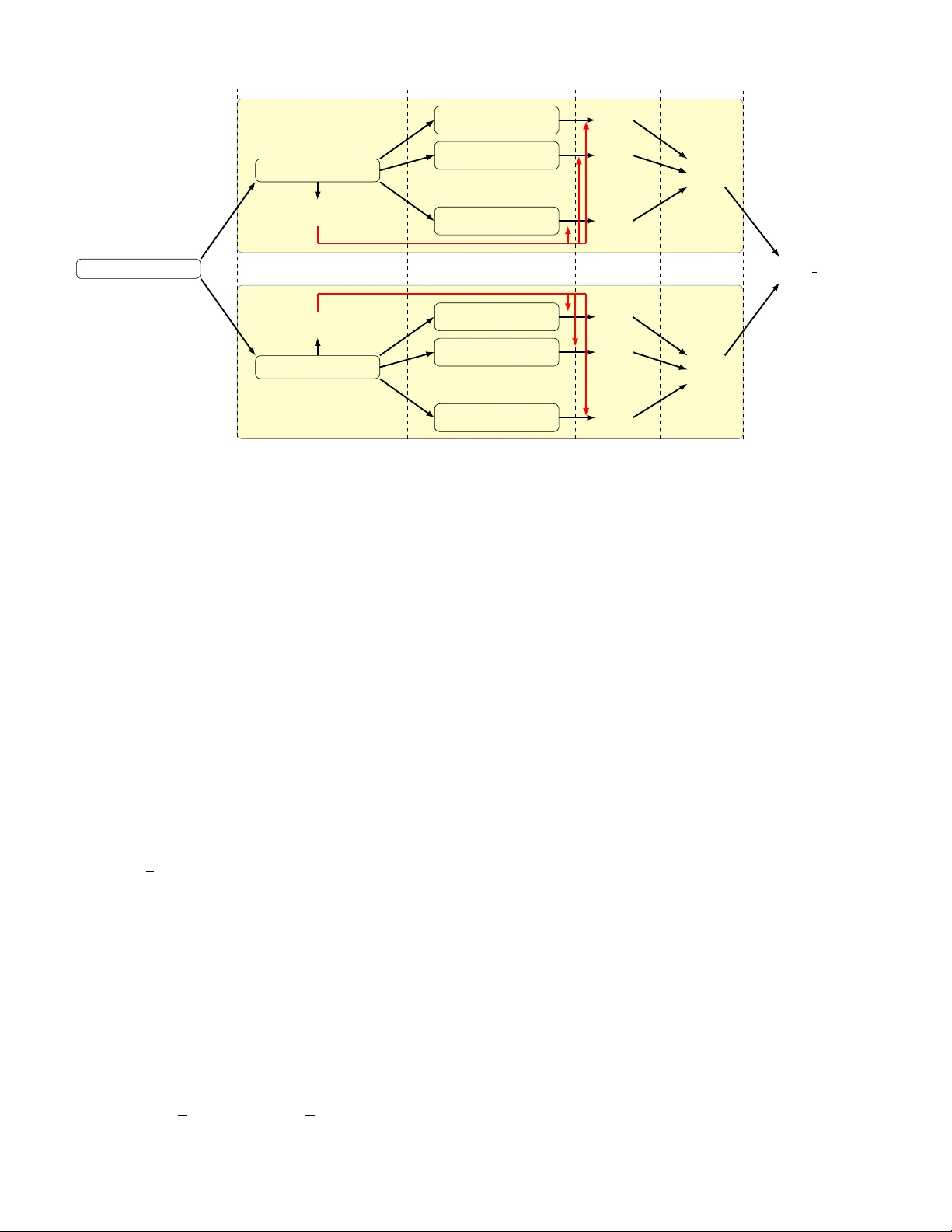
1 Rob ust, scalable and fast bootstrap method for analyzing lar ge scale data Shahab Basiri, Esa Ollila, Member , IEEE, and V isa K oi vunen, F ellow , IEEE Abstract —In this paper we address the problem of perf orming statistical inference for large scale data sets i.e., Big Data. The volume and dimensionality of the data may be so high that it cannot be processed or stor ed in a single computing node. W e propose a scalable, statistically robust and computationally efficient bootstrap method, compatible with distributed pr ocess- ing and storage systems. Bootstrap r esamples are constructed with smaller number of distinct data points on multiple disjoint subsets of data, similarly to the bag of little bootstrap method (BLB) [1]. Then significant sa vings in computation is achieved by av oiding the recomputation of the estimator for each bootstrap sample. Instead, a computationally efficient fixed-point estima- tion equation is analytically solved via a smart appr oximation follo wing the Fast and Robust Bootstrap method (FRB) [2]. Our proposed bootstrap method facilitates the use of highly rob ust statistical methods in analyzing large scale data sets. The fav orable statistical properties of the method are established analytically . Numerical examples demonstrate scalability , low complexity and rob ust statistical performance of the method in analyzing lar ge data sets. Index T erms —bootstrap, bag of little bootstraps, fast and rob ust bootstrap, big data, robust estimation, distributed com- putation. I . I N T RO D U C T I O N R ECENT advances in digital technology have led to a proliferation of large scale data sets. Examples include climate data, social networking, smart phone and health data, etc. Inferential statistical analysis of such large scale data sets is crucial in order to quantify statistical correctness of param- eter estimates and testing hypothesis. Howe ver , the volume of the data has grown to an extent that cannot be ef fectively han- dled by traditional statistical analysis and inferential methods. Processing and storage of massi ve data sets becomes possi- ble through parallel and distributed architectures. Performing statistical inference on massi ve data sets using distributed and parallel platforms require fundamental changes in statistical methodology . Even estimation of a parameter of interest based on the entire massiv e data set can be prohibitively expensiv e. In addition, assigning estimates of uncertainty (error bars, confidence intervals, etc) to the point estimates is not compu- tationally feasible using the con ventional statistical inference methodology such as bootstrap [3]. The bootstrap method is known as a consistent method of assigning estimates of uncertainty (e.g., standard de viation, confidence intervals, etc.) to statistical estimates [3], [4] and it is commonly applied in the field of signal processing [5], [6]. Ho wev er, for at least two obvious reasons the method is computationally impractical for analysis of modern high volume and high-dimensional data sets: F irst , the size of each bootstrap sample is the same as the original big data set (with about 63% of data points appearing at least once in each sam- ple typically), thus leading to processing and storage problems ev en in advanced computing systems. Second , (re)computation of value of the estimator for each massiv e bootstrapped data set is not feasible ev en for estimators with moderate lev el of computational complexity . V ariants such as subsampling [7] and the m out of n bootstrap [8] were proposed to reduce the computational cost of bootstrap by computation of the point estimates on smaller subsamples of the original data set. Implementation of such methods is e ven more problematic as the output is sensitiv e to the size of the subsamples m . In addition extra analytical effort is needed in order to re-scale the output to the right size. The bag of little bootstraps (BLB) [1] modifies the con ven- tional bootstrap to make it applicable for massi ve data sets. In BLB method the massiv e data is subdivided randomly into dis- joint subsets (i.e., so called subsample modules or bags). This allows the massiv e data sets to be stored in distributed fashion. Moreov er subsample modules can be processed in parallel using distributed computing architectures. The BLB samples are constructed by assigning random weights from multino- mial distrib ution to the data points of a disjoint subsample. Although in BLB the problem of handling and processing massiv e bootstrap samples is alleviated, yet (re)computation of the estimates for a large number of bootstrap samples is prohibitiv ely expensi ve. Thus, on the one hand BLB is impractical for many commonly used modern estimators that typically hav e a high complexity . Such estimators often require solving demanding optimization problems numerically . On the other hand, using the primiti ve LS estimator in the original BLB scheme does not provide a statistically robust bootstrap procedure as the LS estimator is kno wn to be very sensitive in the f ace of outliers. In this paper we address the problem of bootstrapping massiv e data sets by introducing a lo w complexity and rob ust bootstrap method. The ne w method possesses similar scala- bility property as the BLB scheme with significantly lower computational complexity . Lo w complexity is achiev ed by utilizing for each subset a fast fixed-point estimation technique stemming from Fast and Robust Bootstrap (FRB) method [2], [9], [10]. It av oids (re)computation of fixed-point equations for each bootstrap sample via a smart approximation. Although the FRB method possesses a lo wer comple xity in comparison with the conv entional bootstrap, the original FRB is incom- patible with distributed processing and storage platforms and it is not suitable for bootstrap analysis of massiv e data sets. Our proposed bootstrap method is scalable and compatible with distrib uted computing architectures and storage systems, robust to outliers and consistently pro vides accurate results in 2 a much faster rate than the original BLB method. W e note that some preliminary results of the proposed approach were presented in the conference paper [11]. The paper is organized as follows. In Section II, the BLB and FRB methods are re viewed. The new bootstrap scheme (BLFRB) is proposed in Section III, followed by implemen- tation of the method for MM-estimator of regression [12]. In Section IV Consistency and statistical robustness of the new method are discussed. Section V provides simulation studies and an e xample of using the ne w method for analysis of a real world big data set. Section VI concludes. I I . R E L A T E D B O OT S T R A P M E T H O D S In this section, we briefly describe the ideas of the BLB [1] and FRB [2] methods. The pros and cons of both methods are discussed as well. A. Bag of Little Bootstraps Let X = ( x 1 · · · x n ) ∈ R d × n be a d dimensional observed data set of size n . The volume and dimensionality of the data may be so high that it cannot be processed or stored in a single node. Consider ˆ θ n ∈ R d as an estimator of a parameter of interest θ ∈ R d based on X . Computation of estimate of uncertainty ˆ ξ ∗ (e.g., confidence intervals, standard deviation, etc,) for ˆ θ n is of great interest as for large data sets confidence intervals are often more informativ e than plain point estimates. The bag of little bootstraps (BLB) [1] is a scalable bootstrap scheme that draws disjoint subsamples ˇ X = ( ˇ x 1 · · · ˇ x b ) ∈ R d × b (which form ”bags” or ”modules”) of smaller size b = {b n γ c | γ ∈ [0 . 6 , 0 . 9] } by randomly resampling without replacement from columns of X . For example if n = 10 7 and γ = 0 . 6 , then b = 15849 . For each subsample module, boot- strap samples, X ∗ , are generated by assigning a random weight vector n ∗ = ( n 1 , . . . , n ∗ b ) from M ultinomial ( n, (1 /b ) 1 b ) to data points of the subsample, where the weights sum to n . The desired estimate of uncertainty ˆ ξ ∗ is computed based on the population ˆ θ ∗ n within each subsample module and the final estimate is obtained by averaging ˆ ξ ∗ ’ s over the modules. In the BLB scheme each bootstrap sample contains at most b distinct data points. Thus the BLB approach produces the bootstrap replicas with reduced ef fort in comparison to con ventional bootstrap [3]. Furthermore, the computation for each subsample can be done in parallel by different computing nodes. Ne vertheless, (re)computing the value of estimator for each bootstrap sample for example thousands of times is still computationally impractical ev en for estimators of moderate lev el of complexity . This includes a wide range of modern estimators that are solutions to optimization problems such as maximum likelihood methods or highly robust estimators of linear re gression. The BLB method was originally introduced with the primitiv e LS estimator . Such combination does not provide a statistically robust bootstrap procedure as the LS estimator is known to be very sensitiv e in the face of outliers. Later in section IV of this paper we sho w that ev en one outlying data point is sufficient to break down the BLB results. B. F ast and Rob ust Bootstrap The fast and robust bootstrap method [2], [9], [10] is computationally efficient and rob ust to outliers in comparison with con ventional bootstrap. It is applicable for estimators ˆ θ n ∈ R d that can be expressed as a solution to a system of smooth fix ed-point (FP) equations: ˆ θ n = Q ( ˆ θ n ; X ) , (1) where Q : R d → R d . The bootstrap replicated estimator ˆ θ ∗ n then solves ˆ θ ∗ n = Q ( ˆ θ ∗ n ; X ∗ ) , (2) where the function Q is same as in (1) but no w dependent on the bootstrap sample X ∗ . Then, instead of computing ˆ θ ∗ n from (2), we compute: ˆ θ 1 ∗ n = Q ( ˆ θ n ; X ∗ ) , (3) where the notation ˆ θ 1 ∗ n denotes an approximation of ˆ θ ∗ n in (2) with initial v alue ˆ θ n based on bootstrap sample X ∗ . In fact ˆ θ 1 ∗ n is a one-step improv ement of the initial estimate. In con ventional bootstrap, one uses the distribution of ˆ θ ∗ n to estimate the sampling distribution of ˆ θ n . Since the distribution of the one-step estimator ˆ θ 1 ∗ n does not accurately reflect the sampling variability of ˆ θ , b ut typically underestimates it, a linear correction needs to be applied as follo ws: ˆ θ R ∗ n = ˆ θ n +  I − ∇Q ( ˆ θ n ; X )  − 1  ˆ θ 1 ∗ n − ˆ θ n  , (4) where ∇Q ( · ) ∈ R d × d is the matrix of partial deriv ativ es w .r .t. ˆ θ n . Then under sufficient regularity conditions, ˆ θ R ∗ n will be estimating the limiting distrib ution of ˆ θ n . In most applications, ˆ θ R ∗ n is not only significantly faster to compute than ˆ θ ∗ n , but numerically more stable and statistically robust as well. Howe ver , the original FRB is not scalable or compatible with distributed storage and processing systems. Hence, it is not suited for bootstrap analysis of massi ve data sets. The method has been applied to man y complex fixed-point estimators such as FastICA estimator [13], PCA and highly rob ust estimators of linear re gression [2]. I I I . F A S T A N D R O B U S T B O O T S T R A P F O R B I G D A TA In this section we propose a new bootstrap method that combines the desirable properties of the BLB and FRB meth- ods. The method can be applied to any estimator representable as smooth FP equations. The de veloped Bag of Little Fast and Rob ust Bootstraps (BLFRB) method is suitable for big data analysis because of its scalability and low computational complexity . Recall that the main computational burden of the BLB scheme is in recomputation of estimating equation (2) for each bootstrap sample X ∗ . Such computational comple xity can be drastically reduced by computing the FRB replications as in (4) instead. This can to be done locally within each bag. Let ˆ θ n,b be a solution to equation (1) for subsample ˇ X ∈ R d × b : ˆ θ n,b = Q ( ˆ θ n,b ; ˇ X ) . (5) Let X ∗ ∈ R d × n be a bootstrap sample of size n randomly resampled with replacement from disjoint subset ˇ X of size 3 Algorithm 1: The BLFRB procedure 1 Draw s subsamples (which form ”bags” or ”modules”) ˇ X = ( ˇ x 1 · · · ˇ x b ) of smaller size b = {b n γ c | γ ∈ [0 . 6 , 0 . 9] } by randomly sampling without replacement from columns of X ; for each subsample ˇ X do 2 Generate r bootstrap samples by resampling as follows: Bootstrap sample X ∗ = ( ˇ X ; n ∗ ) is formed by assigning a random weight vector n ∗ = ( n 1 , . . . , n ∗ b ) from M ultinomial ( n, (1 /b ) 1 b ) to columns of ˇ X ; 3 Find the initial estimate ˆ θ n,b that solves (5) and for each bootstrap sample X ∗ compute ˆ θ R ∗ n,b from equation (6); 4 Compute the desired estimate of uncertainty ˆ ξ ∗ based on the population of r FRB replicated v alues ˆ θ R ∗ n,b ; 5 A verage the computed values of the estimate of uncertainty o ver the subsamples, i.e., ˆ ξ ∗ = 1 s P s k =1 ˆ ξ ∗ ( k ) . b ; or equiv alently generated by assigning a random weight vector n ∗ = ( n 1 , . . . , n ∗ b ) from M ultinomial ( n, (1 /b ) 1 b ) to data points of ˇ X . The FRB replication of ˆ θ n,b can be obtained by ˆ θ R ∗ n,b = ˆ θ n,b +  I − ∇Q ( ˆ θ n,b ; ˇ X )  − 1  ˆ θ 1 ∗ n,b − ˆ θ n,b  , (6) where ˆ θ 1 ∗ n,b = Q ( ˆ θ n,b ; X ∗ ) is the one-step estimator and ∇Q ( · ) ∈ R d × d is the matrix of partial deriv ativ es w .r .t. ˆ θ n,b . The proposed BLFRB procedure is giv en in detail in Algorithm 1 . The steps of the algorithm are illustrated in Fig. 1 , where ˇ X ( k ) , k = 1 , . . . , s denotes the disjoint subsamples and X ∗ ( kj ) corresponds to the j th bootstrap sample generated from the distinct subsample k . Note that the terms ˆ θ n,b and  I − ∇Q ( ˆ θ n,b ; ˇ X )  − 1 are computed only once for each bag. While the BLFRB procedure inherits the scalability of BLB, it is radically faster to compute, since the replication ˆ θ R ∗ n,b can be computed in closed-form with small number of distinct data points. Low complexity of the BLFRB scheme allows for fast and scalable computation of confidence intervals for commonly used modern fixed-point estimators such as FastICA estimator [13], PCA and highly rob ust estimators of linear regression [2]. A. BLFRB for MM-estimator of linear r egr ession Here we present a practical example formulation of the method, where the proposed BLBFR method is used for linear regression. In order to construct a statistically robust bootstrap method, MM-estimator that lends itself to fixed point estimation equations is employed for bootstrap replicas. Let X = { ( y 1 , z > 1 ) > , . . . , ( y n , z > n ) > } , z i ∈ R p , be a sample of independent random v ectors that follo w the linear model: y i = z > i θ + σ 0 e i for i = 1 , . . . , n, (7) where θ ∈ R p is the unknown parameter v ector . Noise terms e i ’ s are i.i.d. random variables from a symmetric distrib ution with unit scale. Highly robust MM-estimators [12] are based on two loss functions ρ 0 : R → R + and ρ 1 : R → R + which determine the breakdown point and ef ficiency of the estimator , respecti vely . The ρ 0 ( · ) and ρ 1 ( · ) functions are symmetric, twice continu- ously differentiable with ρ (0) = 0 , strictly increasing on [0 , c ] and constant on [ c, ∞ ) for some constant c . The MM-estimate of ˆ θ n satisfies 1 n n X i =1 ρ 0 1  y i − z > i ˆ θ n ˆ σ n  z i = 0 (8) where ˆ σ n is a S-estimate [14] of scale. Consider M-estimate of scale ˆ s n ( θ ) defined as a solution to 1 n n X i =1 ρ 0  y i − z > i θ ˆ s n ( θ )  = m, (9) where m = ρ 0 ( ∞ ) / 2 is a constant. Let ˜ θ n be the argument that minimizes ˆ s n ( θ ) , ˜ θ n = arg min θ ∈ R p ˆ s n ( θ ) , then ˆ σ n = ˆ s n ( ˜ θ n ) . W e employ the T ukey’ s loss function: ρ e ( u ) = ( u 2 2 − u 4 2 c 2 e + u 6 6 c 4 e for | u | ≤ c e c 2 e 6 for | u | > c e , which is widely used as the ρ functions of the MM-estimator, where subscript e represents different tunings of the function. For instance an MM-estimator with efficienc y O = 95% and breakdown point B P = 50% (i.e. for Gaussian errors) is achiev able by tuning ρ e ( u ) into c 0 = 1 , 547 and c 1 = 4 , 685 for ρ 0 and ρ 1 respectiv ely (see [15, p.142, tab .19]). In this paper (8) is computed using an iterativ e algorithm proposed in [16]. The initial v alues of iteration are obtained from (9) which in turns are computed using the F astS algorithm [17]. In order to apply the BLFRB method to MM-estimator, (8) and (9) need to be presented in form of FP equations scalable to number of distinct data points in the data. The corresponding scalable one-step MM-estimates ˆ θ 1 ∗ n and ˆ σ 1 ∗ n are obtained by modifying [2, eq. 17 and 18] as follows. Let X ∗ = ( ˇ X ; n ∗ ) denote a BLB bootstrap sample based on subsample ˇ X = { ( ˇ y 1 , ˇ z > 1 ) > , . . . , ( ˇ y b , ˇ z > b ) > } , ˇ z i ∈ R p and a weight vector n ∗ = ( n ∗ 1 · · · n ∗ b ) ∈ R b , ˆ θ 1 ∗ n =  b X i =1 n ∗ i ˇ ω i ˇ z i ˇ z > i  − 1 b X i =1 n ∗ i ˇ ω i ˇ z i ˇ y i , (10) ˆ σ 1 ∗ n = b X i =1 n ∗ i ˇ υ i ( ˇ y i − ˇ z > i ˜ θ n ) , (11) where ˇ r i = ˇ y i − ˇ z > i ˆ θ n , ˜ r i = ˇ y i − ˇ z > i ˜ θ n , ˇ ω i = ρ 0 1 ( ˇ r i / ˆ σ n ) / ˇ r i and ˇ υ i = ˆ σ n nm ρ 0 ( ˜ r i / ˆ σ n ) / ˜ r i . 4 X = ( x 1 · · · x n ) step: 1 ˇ X (1) = ( ˇ x (1) 1 · · · ˇ x (1) b ) ˇ X ( s ) = ( ˇ x ( s ) 1 · · · ˇ x ( s ) b ) ˆ θ (1) n,b ˆ θ ( s ) n,b step: 2 X ∗ (11) = ( ˇ X (1) ; n ∗ (11) ) X ∗ (12) = ( ˇ X (1) ; n ∗ (12) ) . . . X ∗ (1 r ) = ( ˇ X (1) ; n ∗ (1 r ) ) . . . X ∗ ( s 1) = ( ˇ X ( s ) ; n ∗ ( s 1) ) X ∗ ( s 2) = ( ˇ X ( s ) ; n ∗ ( s 2) ) . . . X ∗ ( sr ) = ( ˇ X ( s ) ; n ∗ ( sr ) ) step: 3 ˆ θ R ∗ (11) n,b ˆ θ R ∗ (12) n,b . . . ˆ θ R ∗ (1 r ) n,b ˆ θ R ∗ ( s 1) n,b ˆ θ R ∗ ( s 2) n,b . . . ˆ θ R ∗ ( sr ) n,b step: 4 ˆ ξ ∗ (1) ˆ ξ ∗ ( s ) step: 5 ˆ ξ ∗ = 1 s P s i =1 ˆ ξ ∗ ( i ) Fig. 1. The steps of the BLFRB procedure ( Algorithm 1 ) are depicted. Disjoint subsamples of significantly smaller size b are drawn from the original Big Data set X . The initial estimate ˆ θ n,b is obtained by solving fixed-point estimating equation only once for each subsample ˇ X . Within each module, the FRB replicas ˆ θ R ∗ n,b are computed for each bootstrap sample X ∗ using the initial estimate ˆ θ n,b . The final estimate of uncertainty ˆ ξ ∗ is obtained by averaging the results of distinct subsample modules. The BLFRB replications of ˆ θ n , are obtained by applying the FRB linear correction as in [2, eq. 20], to the one-step estimators of (10) and (11). I V . S TA T I S T I C A L P RO P E RT I E S Next we establish the asymptotic conv ergence and statistical robustness of the proposed BLFRB method. A. Statistical Con ver gence W e sho w that the asymptotic distribution of BLFRB replicas in each bag is the same as the con ventional bootstrap. Let X = { x 1 , . . . , x n } be a set of observed data as the outcome of i.i.d. random v ariables X = { X 1 , . . . , X n } from an unknown distrib ution P . The empirical distribution (measure) formed by X is denoted by linear combination of the Dirac measures at the observ ations P n = n − 1 P n i =1 δ x i . Let P ( k ) n,b = n − 1 P b i =1 n b δ ˇ x ( k ) i and P ∗ n,b = n − 1 P n i =1 δ x ∗ i denote the em- pirical distrib utions formed by subsample ˇ X ( k ) and bootstrap sample X ∗ respectiv ely . W e also use φ ( · ) for functional rep- resentations of the estimator e.g., θ = φ ( P ) , ˆ θ ( k ) n,b = φ ( P ( k ) n,b ) and ˆ θ ∗ n,b = φ ( P ∗ n,b ) . The notation d = denotes that both sides hav e the same limiting distribution. Theor em 4.1: Consider P , P n and P ( k ) n,b as maps from a Donsker class F to R such that F δ = { f − g : f , g ∈ F , { P ( f − P f ) 2 } 1 / 2 < δ } is measurable for e very δ > 0 . Let φ to be Hadamard differentiable at P tangentially to some subspace and ˆ θ n be a solution to a system of smooth FP equations. Then as n, b → ∞ √ n ( ˆ θ R ∗ n,b − ˆ θ ( k ) n,b ) d = √ n ( ˆ θ n − θ ) . (12) See the proof in the Appendix. B. Statistical r obustness Consider the linear model (7) and let ˆ θ n be an estimator of the parameter vector θ based on X . Let q t , t ∈ (0 , 1) , denote the t th upper quantile of [ ˆ θ n ] l , where [ ˆ θ n ] l is the l th element of ˆ θ n , l = 1 , . . . , p . In other words P r  [ ˆ θ n ] l > q t  = t . Here we study the rob ustness properties of BLB and BLFRB estimates of q t . W e only focus on the robustness properties of one bag as it is easy to see that the end results of both methods break do wn, if only one bag produces a corrupted estimate. Let ˆ q ∗ t denote the BLB or BLFRB estimate of the q t based on a random subsample ˇ X of size b = {b n γ c | γ ∈ [0 . 6 , 0 . 9] } drawn from a big data set X . Follo wing [18], we define the upper breakdown point of ˆ q ∗ t as the minimum proportion of asymmetric outlier contamination in subsample ˇ X that can driv e ˆ q ∗ t ov er any finite bound. Theor em 4.2: In the original BLB setting with LS estimator , only one outlying data point in a subsample ˇ X is sufficient to driv e ˆ q ∗ t , t ∈ (0 , 1) ov er any finite bound and hence, ruining the end result of the whole scheme. See the proof in the Appendix. Let X = { ( y 1 , z > 1 ) > , . . . , ( y n , z > n ) > } , be an observed data set follo wing the linear model (7). Assume that the explanatory variables z i ∈ R p are in general position [15, p. 117]. Let ˆ θ n be an MM-estimate of θ based on X . According to [10, Theorem 2], the FRB estimate of the t th quantile of [ ˆ θ n ] l remains bounded as far as ˆ θ n in equation (1) is a reliable estimate of θ and more than (1 − t )% of the bootstrap samples contain at least p good (i.e., non-outlying) data points. This means that in FRB, higher quantiles are more robust than the lower ones. Here we sho w that in a BLFRB bag the former condition guarantees the latter . Theor em 4.3: Let ˇ X = { ( ˇ y 1 , ˇ z > 1 ) > , . . . , ( ˇ y b , ˇ z > b ) > } , be a 5 T ABLE I U P PE R B R EA K D OW N P O I NT O F T H E B L FR B E S TI M A T E S O F Q UA N T I LE S F O R M M - R E G R ES S I ON E S T IM ATO R W I T H 50% B RE A K DO W N P O IN T A N D 95% EFFI C I E NC Y A T T H E G AU S SI A N M O D E L . p n γ = 0 . 6 γ = 0 . 7 γ = 0 . 8 50 50000 0.425 0.475 0.491 200000 0.467 0.490 0.497 1000000 0.488 0.497 0.499 100 50000 0.349 0.449 0.483 200000 0.434 0.481 0.494 1000000 0.475 0.494 0.498 200 50000 0.197 0.398 0.465 200000 0.368 0.461 0.488 1000000 0.450 0.487 0.497 subsample of size b = {b n γ c | γ ∈ [0 . 6 , 0 . 9] } randomly drawn from X following the linear model (7). Assume that the explanatory v ariables ˇ z > 1 , . . . , ˇ z > b ∈ R p are in general position. Let ˆ θ n,b be an MM-estimator of θ based on ˇ X and let δ b be the finite sample breakdown point of ˆ θ n,b . Then in the BLFRB bag formed by ˇ X , all the estimated quantiles ˆ q ∗ t , t ∈ (0 , 1) hav e the same breakdown point equal to δ b . See the proof in the Appendix. Theorem 4.3 implies that in the BLFRB setting, lower quan- tiles are as rob ust as higher ones with breakdo wn point equal to δ b which can be set close to 0.5. This provides the maximum possible statistical rob ustness for the quantile estimates. In the proof we sho w that if ˆ θ n,b is a reliable MM-estimate of θ , then all the bootstrap samples of size n dra wn from ˇ X are constrained to ha ve at least p good data points. T able 1 illustrates the upper breakdown points of the BLFRB estimates of quantiles for various dimensions of data and different subsample sizes. The MM-regression estimator is tuned into 50% breakdo wn point and 95% ef ficiency at the central model. The results rev eal that BLFRB is significantly more robust than the original BLB with LS estimator . Another important outcome of the table is that, when choosing the size of subsamples b = n γ , the dimension p of the data should be taken into account; For example for a data set of size n = 50000 and p = 200 , setting γ = 0 . 6 or 0 . 7 are not the right choices. V . N U M E R I C A L E X A M P L E S In this section the performance of the BLFRB method is as- sessed by simulation studies. W e also perform the simulations with the original BLB method for comparison purposes. A. Simulation studies W e generate a simulated data set X = { ( y 1 , z > 1 ) > , . . . , ( y n , z > n ) > } of size n = 50000 following the linear model y i = z > i θ + σ 0 e i , ( i = 1 , . . . , n ) , where the explaining variables z i are generated from p -variate normal distribution N p ( 0 , I p ) with p = 50 , p -dimensional parameter vector θ = 1 p , noise terms are i.i.d. from the standard normal distribution and noise variance is σ 2 0 = 0 . 1 . The MM-estimator in the BLFRB scheme is tuned to ha ve efficienc y O = 95% and breakdown point B P = 50% . The -3 -2 -1 0 1 2 3 CDF 0 0.2 0.4 0.6 0.8 1 True CDF Worst CDF (BLFRB) Best CDF (BLFRB) Fig. 2. The true distribution of the right hand side of (12) along with the obtained empirical distributions of the left hand side for two elements of ˆ θ R ∗ n,b with the best and the worst estimates. -3 -2 -1 0 1 2 3 CDF 0 0.2 0.4 0.6 0.8 1 True CDF Ave. CDF (BLFRB) Fig. 3. The av erage of all p BLFRB estimated distributions, along with the true distribution. Note that the averaged empirical distribution conver ge to the true cdf. This confirms the results of theorem 4.1. original BLB scheme in [1] uses LS-estimator for computation of the bootstrap estimates of θ . Here, we first verify the result of theorem 4.1 in simulation by comparing the distribution of the left hand side of (12) with the right hand side. Giv en the abov e settings, the right hand side of (12) follows N p ( 0 , σ 2 0 / O I p ) in distribution [12, theorem 4.1]. W e form the distribution of the left hand side, by drawing a random subsample ˇ X of size b =  50000 0 . 7  = 1946 and performing steps 2 and 3 of the BLFRB procedure (i.e., Algorithm 1 ) for ˇ X using r = 1000 bootstrap samples. Fig.2 sho ws the true distribution of √ n ( ˆ θ n − θ ) along with the obtained empirical distributions of √ n ( ˆ θ R ∗ n,b − ˆ θ n,b ) for two elements of ˆ θ R ∗ n,b with the best and the worst outcomes. The result of a veraging all the p empirical distrib utions is illustrated in Fig.3 , along with the true distribution. Note that the results are in conformity with theorem 4.1. Next, we compare the performance of the BLB and BLFRB methods. W e compute bootstrap estimate of standard deviation (SD) of ˆ θ n by the two methods. In other words, the estimate of uncertainty in step 4 of the procedure (i.e., see Fig.1 ) for bag k is as follo ws: ˆ ξ ∗ ( k ) l = c SD([ ˆ θ ( k ) n,b ] l ) = r X j =1  [ ˆ θ ∗ ( kj ) n,b ] l − [ ˆ θ ∗ ( k · ) n,b ] l  2 r − 1 ! 1 / 2 , 6 No. bootstrap samples (r) 0 50 100 150 200 250 300 Relarive errors ( ε ) 0 0.05 0.1 0.15 0.2 0.25 BLB BLFRB Fig. 4. Relati ve errors of the BLB (dashed line) and BLFRB (solid line) methods w .r .t. the number of bootstrap samples r are illustrated. Both methods perform equally well when there are no outliers in the data. where [ ˆ θ n,b ] l denotes the l th element of ˆ θ n,b and [ ˆ θ ∗ ( k · ) n,b ] l = 1 r P r j =1 [ ˆ θ ∗ ( kj ) n,b ] l . The step 5 of the procedure for the l th element of ˆ θ n,b is obtained by: ˆ ξ ∗ l = c SD([ ˆ θ n ] l ) = 1 s s X k =1 c SD([ ˆ θ ( k ) n,b ] l ) , l = 1 , . . . , p. The performance of the BLB and BLFRB are assessed by computing a relati ve error defined as: ε =    c SD( ˆ θ n ) − SD o ( ˆ θ n )    SD o ( ˆ θ n ) , where c SD( ˆ θ n ) = 1 p P p l =1 c SD([ ˆ θ n ] l ) and SD o ( ˆ θ n ) = σ 0 / √ n O is (approximation of) the av erage standard deviation of ˆ θ n based on the asymptotic cov ariance matrix [12] (i.e., O is 0.95 for the MM-estimator and 1 for the LS-estimator). The bootstrap setup is as follows; Number of disjoint subsamples is s = 25 , size of each subsample is b = b n γ c = 1946 with γ = 0 . 7 , maximum number of bootstrap samples in each subsample module is r max = 300 . W e start from r = 2 and continually add a new set of bootstrap samples (while r < r max ) to subsample modules. The con vergence of relati ve errors w .r .t. the number of bootstrap samples r are illustrated in Fig.4 . Note that when the data is not contaminated by outliers, both methods perform similarly in terms of achieving lower lev el of relativ e errors for higher number of bootstrap samples. W e study the robustness properties of the methods using the abov e settings. According to theorem 4.2, only one outlying data point is suf ficient to driv e the BLB estimates of c SD( ˆ θ n ) ov er any finite bound. T o introduce such outlier , we randomly choose one of the original data points and multiply it by a large number α . Such contamination scenario resembles misplacement of the decimal point in real world data sets. Lack of robustness of the BLB method is illustrated in Fig.5a for α = 500 and α = 1000 . According to T able 1 , for the settings of our example the upper breakdo wn point of BLFRB quantile estimates is δ b = 0 . 475 . Let us asses the statistical robustness of the BLFRB scheme by sev erely contaminating the original data No. bootstrap samples (r) 0 50 100 150 200 250 300 Relarive errors ( ε ) 0 2 4 6 BLB, α = 1000 BLB, α = 500 BLB, Clean data (a) No. bootstrap samples (r) 0 50 100 150 200 250 300 Relarive errors ( ε ) 0 2 4 6 BLFRB, α = 1000 BLFRB, Clean data (b) Fig. 5. (a) Relative errors of the BLB method illustrating severe lack of robustness in face of only one outlying data point. (b) Relative errors of the BLFRB method illustrating the reliable performance of the method in the face of severely contaminated data. points of the first bag. W e multiply 40% ( b 0 . 4 × b c = 778 ) of the data points by α = 1000 . As sho wn in Fig.5b , BLFRB still performs highly robust despite such proportion of outlying data points. Now , let us make an intuitive comparison between com- putational complexity of the BLB and BLFRB methods by using the MM-estimator in both methods. W e use an identical computing system to compute bootstrap standard de viation (SD) of ˆ θ n by the two methods. The computed ε and the cumulativ e processing time are stored after each iteration (i.e.,adding new set of bootstrap samples to the bags). Fig.6 , reports relativ e errors w .r .t. the required cumulative processing time after each iteration of the algorithms. The BLFRB is remarkably faster since the method av oids solving estimating equations for each bootstrap sample. B. Real world data Finally , we use the BLFRB method for bootstrap analysis of a real lar ge data set. W e consider the simplified v ersion of the the Million Song Dataset (MSD) [19], av ailable on the UCI Machine Learning Repository [20]. The data set X = { ( y 1 , z > 1 ) > , . . . , ( y n , z > n ) > } contains n = 515345 music tracks, where y i (i.e., i = 1 , . . . , n ) represents the released year of the i th song (i.e., ranging from 1922 to 2011) and z i ∈ R p is a vector of p = 90 different audio features of each 7 Processing Time(Sec.) 0 2000 4000 6000 8000 Relative errors ( ε ) 0 0.05 0.1 0.15 0.2 0.25 BLB BLFRB Fig. 6. Relati ve errors ε w .r.t. the required processing time of each BLB and BLFRB iteration. The BLFRB is significantly faster to compute as the (re)computation of the estimating equations is not needed in this method. song. The used features are the average and non-redundant cov ariance v alues of the timbre v ectors of the song. The linear regression can be used to predict the released year of a song based on its audio features. W e use the BLFRB method to conduct a fast, robust and scalable bootstrap test on the regression coefficients. In other words, considering the linear model y i = z > i θ + σ 0 e i , we use BLFRB for testing hypothesis H 0 : b θ c l = 0 vs. H 1 : b θ c l 6 = 0 , where b θ c l (i.e., l = 1 , . . . , p ) denotes the l th element of θ . The BLFRB test of lev el α rejects the null hypothesis if the computed 100(1 − α )% confidence interval does not contain 0 . Here we run the BLFRB hypothesis test of level α = 0 . 05 with the following bootstrap setup; Number of disjoint subsamples is s = 51 , size of each subsample is b = b n γ c = 9964 with γ = 0 . 7 , number of bootstrap samples in each subsample module is r = 500 . Among all the 90 features, the null hypothesis is accepted only for 6 features numbered: 32 , 40 , 44 , 47 , 54 , 75 . Fig.7 shows the computed 95% CIs of the features. In order to provide a closer view , we hav e only shown the results for feature numbers 30 to 80. These results can be exploited to reduce the dimension of the data by excluding the ineffecti ve variables from the regression analysis. Using the BLFRB method with the highly robust MM- estimator , we ensure that the computational process is done in a reasonable time frame and the results are not af fected by possible outliers in the data. Such desirable properties are not offered by the other methods considered in our comparisons. V I . C O N C L U S I O N In this paper, a new robust, scalable and low complexity bootstrap method is introduced with the aim of finding param- eter estimates and confidence measures for very large scale data sets. The statistical properties of the method including con vergence and robustness are established using analytical methods. While the proposed BLFRB method is fully scalable and compatible with distributed computing systems, it is re- markably faster and significantly more rob ust than the original BLB method [1]. A P P E N D I X A Here we provide the proofs of the theoretical results of sections IV -A and IV -B. Feature Number 30 35 40 45 50 55 60 65 70 75 80 95% CI -0.1 -0.05 0 0.05 0.1 Rejected H 0 Accepted H 0 Fig. 7. The 95% confidence intervals computed by BLFRB method is shown for some of the audio features of the MSD data set. The null hypothesis in accepted for those features having 0 inside the interval. Proof of theor em 4.1 : Giv en that F is Donsker class, as n → ∞ : G n = √ n ( P n − P ) d → G p , (13) where G p is the P-Br ownian bridge pr ocess and the notation d → denotes conv ergence in distribution. According to [21, theorem 3.6.3] as b, n → ∞ : G ∗ n,b = √ n ( P ∗ n,b − P ( k ) n,b ) d → G p . (14) Thus, G n and G ∗ n,b con verge in distribution to the same limit. The functional delta method for bootstrap [22, theorem 23.9] in conjunction with [23, lemma 1] imply that, for ev ery Hadamard-differentiable function φ : √ n ( φ ( P n ) − φ ( P )) d → φ 0 P ( G p ) , (15) and conditionally on P ( k ) n,b , √ n ( φ ( P ∗ n,b ) − φ ( P ( k ) n,b )) d → φ 0 P ( G p ) , (16) where φ 0 P ( G p ) is the deri vati ve of φ w .r .t. P at G p . Thus, conditionally on P ( k ) n,b , √ n ( ˆ θ ∗ n,b − ˆ θ ( k ) n,b ) d = √ n ( ˆ θ n − θ ) . (17) According to [2, equation 5 and 6] and giv en that ˆ θ n can be expressed as a solution to a system of smooth FP equations: √ n ( ˆ θ R ∗ n,b − ˆ θ ( k ) n,b ) d = √ n ( ˆ θ ∗ n,b − ˆ θ ( k ) n,b ) . (18) Form (17) and (18): √ n ( ˆ θ R ∗ n,b − ˆ θ ( k ) n,b ) d = √ n ( ˆ θ n − θ ) (19) which concludes the proof.  The follo wing lemma is needed to pro ve theorems 4.2 and 4.3. Lemma 1: Let ˇ X = ( ˇ x 1 · · · ˇ x b ) be a subset of size b = {b n γ c | γ ∈ [0 . 6 , 0 . 9] } randomly resampled without replace- ment from a big data set X of size n . Let X ∗ be a bootstrap sample of size n randomly resampled with replacement from ˇ X (i.e., or equi valently formed by assigning a random weight vector n ∗ = ( n 1 , . . . , n ∗ b ) from M ultinomial ( n, (1 /b ) 1 b ) to columns of ˇ X ). Then: lim n →∞ P r { ˇ x ( i ) / ∈ X ∗ | for an y ˇ x ( i ) ∈ ˇ X } → 0 . 8 Proof of lemma 1 : Consider an arbitrary data point ˇ x ( i ) ∈ ˇ X . The probability that ˇ x ( i ) does not occur in a bootstrap sample of size n → ∞ is: lim n →∞ P r ( B inomial ( n, 1 n γ ) < 1) = lim n →∞ (1 − 1 n γ ) n = lim n →∞ exp  ln(1 − 1 n γ ) 1 /n  = lim n →∞ exp  − γ n 2 n γ +1 − n  = 0 .  Such probability for n = 20000 and γ = 0 . 7 is 3 . 3 × 10 − 9 . Proof of theorem 4.2 : Let ˇ x ( i ) ∈ ˇ X be an outlying data point in ˇ X . According to lemma 1, all bootstrap samples drawn from that subsample will be contaminated by ˇ x ( i ) . This is sufficient to break all the LS replicas of the estimator in that bag and consequently ruining the end result of the whole scheme.  Proof of theorem 4.3 : According to [10, Theorem 2], The FRB estimate of q t remains bounded as far as: 1. ˆ θ n in equation (1) is a reliable estimate of θ , and 2. More than (1 − t )% of the bootstrap samples contain at least p ”good” (i.e., non-outlying) data points. The first condition implies that, in a BLFRB bag if ˆ θ n,b is a corrupted estimate then all bootstrap estimates ˆ q ∗ t , t ∈ (0 , 1) will break as well. In the rest of the proof we show that if the percentage of outliers in ˇ X is such that ˆ θ n,b is still a reliable estimate of θ , then all the bootstrap samples drawn from ˇ X contain at least p good (non-outlying) data points. This suf fices for all ˆ q ∗ t , t ∈ (0 , 1) to remain bounded. Let ˆ θ n,b be an MM-estimate of θ . Let the initial scale of the MM-estimator obtain by a high breakdo wn point S-estimator . The finite sample breakdo wn point of the S-estimator for a subsample of size b is as follo ws: δ S b = b b/ 2 c − p + 2 b , [15, Theorem 8]. Giv en that ˆ θ n,b is a reliable estimate, the initial S-estimate of the scale parameter is not broken. This implies that there exist at least h = b − b b/ 2 c + p − 1 good data points in general position in ˇ X . It is easy to see that h > p . Applying Lemma 1 for each of the good points concludes that the probability of drawing a bootstrap sample of size n with less than p good data points goes to zero for large n , which is the case of big data sets.  R E F E R E N C E S [1] A. Kleiner, A. T alwalkar , P . Sarkar , and M. I. Jordan, “ A scalable bootstrap for massiv e data, ” Journal of the Royal Statistical Society: Series B (Statistical Methodology) , v ol. 76, no. 4, pp. 795–816, 2014. [2] M. Salibi ´ an-Barrera, S. V an Aelst, and G. Willems, “F ast and robust bootstrap, ” Statistical Methods and Applications , vol. 17, no. 1, pp. 41– 71, 2008. [3] B. Efron and R. J. T ibshirani, An intr oduction to the bootstrap . CRC press, 1994. [4] A. C. Davison, Bootstrap methods and their application , vol. 1. Cam- bridge university press, 1997. [5] A. Zoubir and D. Iskander , Bootstrap T echniques for Signal Processing . Cambridge University Press, 2004. [6] A. Zoubir and B. Boashash, “The bootstrap and its application in signal processing, ” Signal Pr ocessing Magazine, IEEE , vol. 15, pp. 56–76, Jan 1998. [7] M. W . Dimitris N. Politis, Joseph P . Romano, Subsampling . Springer, 1999. [8] P . J. Bickel, F . G ¨ otze, and W . R. van Zwet, Resampling fewer than n observations: gains, losses, and r emedies for losses . Springer , 2012. [9] M. Salibi ´ an-Barrera, Contributions to the theory of rob ust inference . PhD thesis, Citeseer, 2000. [10] M. Salibian-Barrera and R. H. Zamar, “Bootstrapping robust estimates of regression, ” Annals of Statistics , pp. 556–582, 2002. [11] S. Basiri, E. Ollila, and V . Koivunen, “Fast and robust bootstrap in analysing large multiv ariate datasets, ” in Asilomar Conference on Signals, Systems and Computers , pp. 8–13, IEEE, 2014. [12] V . J. Y ohai, “High breakdown-point and high efficiency robust estimates for regression, ” The Annals of Statistics , pp. 642–656, 1987. [13] S. Basiri, E. Ollila, and V . Koivunen, “Fast and robust bootstrap method for testing hypotheses in the ica model, ” in Acoustics, Speech and Signal Pr ocessing (ICASSP), 2014 IEEE International Conference on , pp. 6– 10, IEEE, 2014. [14] P . Rousseeuw and V . Y ohai, “Robust regression by means of s- estimators, ” in Robust and nonlinear time series analysis , pp. 256–272, Springer , 1984. [15] P . J. Rousseeuw and A. M. Leroy , Robust r egr ession and outlier detection , vol. 589. John Wile y & Sons, 2005. [16] C. Croux, G. Dhaene, and D. Hoorelbeke, “Robust standard errors for robust estimators, ” CES-Discussion paper series (DPS) 03.16 , pp. 1–20, 2004. [17] M. Salibian-Barrera and V . J. Y ohai, “ A fast algorithm for s-regression estimates, ” J ournal of Computational and Gr aphical Statistics , vol. 15, no. 2, 2006. [18] K. Singh et al. , “Breakdown theory for bootstrap quantiles, ” The annals of Statistics , vol. 26, no. 5, pp. 1719–1732, 1998. [19] T . Bertin-Mahieux, D. P . Ellis, B. Whitman, and P . Lamere, “The million song dataset, ” in Pr oceedings of the 12th International Conference on Music Information Retrieval (ISMIR 2011) , 2011. [20] M. Lichman, “UCI machine learning repository , ” 2013. [21] A. W . V an Der V aart and J. A. W ellner, W eak Con vergence . Springer, 1996. [22] A. W . V an der V aart, Asymptotic statistics , vol. 3. Cambridge univ ersity press, 1998. [23] A. Kleiner, A. T alwalkar , P . Sarkar , and M. I. Jordan, “ A scalable bootstrap for massive data supplementary material, ” 2013.