Locally Imposing Function for Generalized Constraint Neural Networks - A Study on Equality Constraints

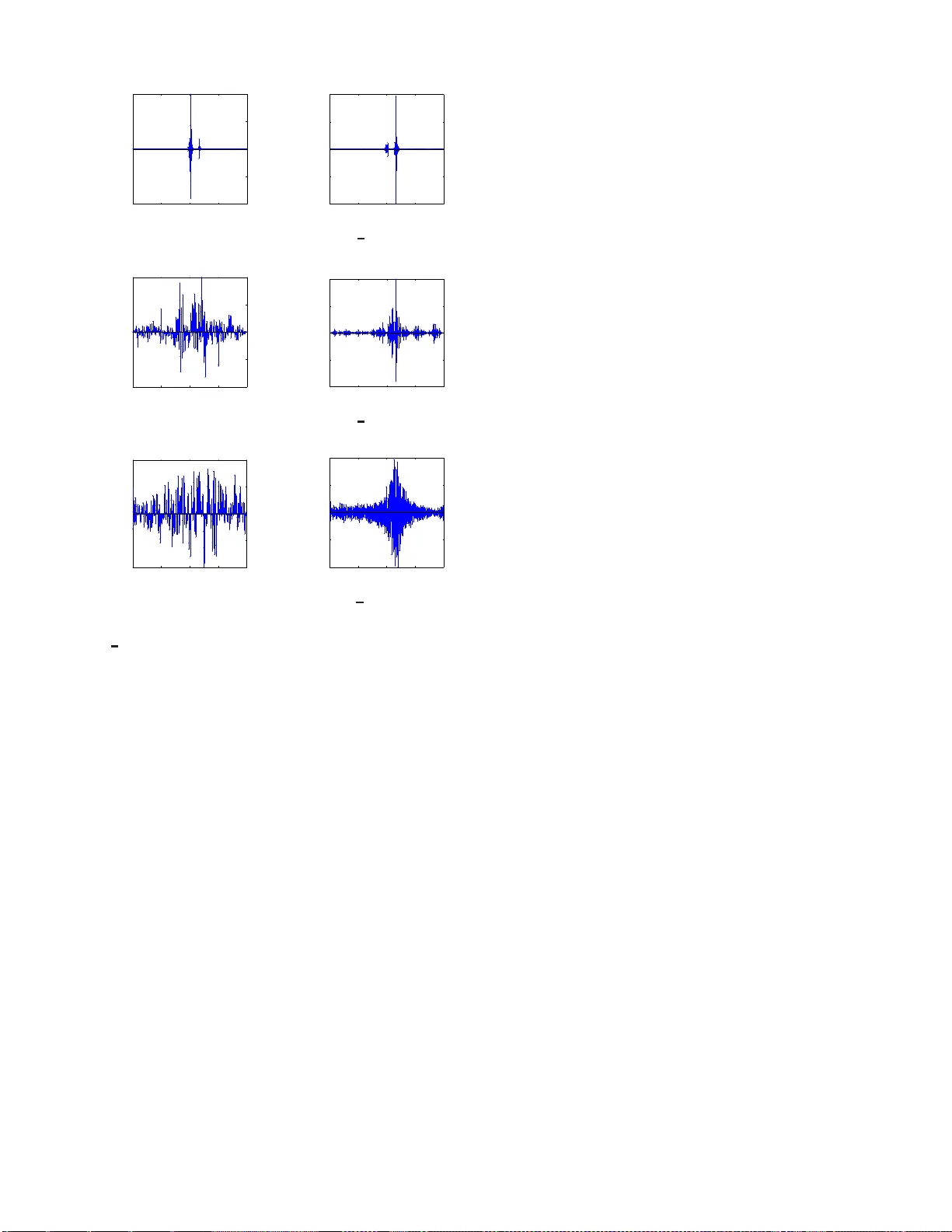
Locally Imposing Function for Generalized Constraint Neural Networks - A Study on Equ ality Constraints Linlin Cao NLPR, Institute of Automa tion Chinese Academy of Sciences Beijing, China Email: linlincao nlpr@ 163 .com Ran He NLPR, Institute of Automa tion Chinese Academy of Sciences Beijing, China Email: rhe@nlpr .ia.ac.cn Bao-Gang Hu NLPR, Institute of Automa tion Chinese Academy of Sciences Beijing, China Email: hubg@nlpr .ia.ac.cn Abstract —This work is a furth er study on the Generalized Constraint Ne ural Netw ork (GCNN) model [1], [2]. T w o chal- lenges are encountered in the study , that is, to embed any type of prior inf ormation and to s elect its imposing schemes. The work fo cuses on th e second challenge and stud ies a new constraint imposing scheme for equ ality constraint s. A new method called locally imposing functi on (LIF) is proposed to provide a local correc tion to the GCNN prediction function, which therefor e falls within Locally Imposing Scheme (LIS). In comparison, the con ventional Lagrange multip lier method is considered as Globally Imposing Scheme (GIS) because its added constraint term exhibits a global impact to its objective functi on. T wo advantages are gained from LIS ov er GIS. Fi rst, LIS enables constraints to fire locally and explicitly in the d omain only where they need on t he prediction function. Second, constraints can be implemented within a netwo rk setting directly . W e attempt to inter pret sev eral constraint methods graphically from a viewp oint of the locality princip le. Numerical examples confirm the advantages of the proposed method. In solving bound ary value pro blems with Dirichlet and Neumann constraints, the GCNN model with LIF is possible to achiev e an exact satisfaction of the constraints. I . I N T RO D U C T I O N Artificial neu ral networks ( ANNs ) hav e rec ei ved sign ificant progr esses after the propo sal o f deep learning models [3]– [5]. ANNs a re fo rmed main ly b ased on learn ing fro m d ata. Hen ce, they a re considered as d ata-driven ap proach [6] with a black- box limitatio n [7]. While this feature provides a flexiblility power to ANNs in mo deling, they miss a f unctionin g part for top -down mechanisms , which seems to be necessary for realizing h uman-like m achines. Furth ermore, the ultimate goal of machine learning stu dy is insight, not machine itself. Th e current ANNs, includ ing deep learning mo dels, fail to present interpretatio ns about their lear ning processes as well as the associated p hysical targets, su ch as human brains. For ad ding tran sparency to ANNs, we prop osed a g ener- alized constra int neural network ( GCNN ) appro ach [ 1], [8], [9]. I t can also be viewed a s a knowledge-an d-data -driven modeling ( KDDM ) ap proach [10], [11] b ecause two sub mod- els a re fo rmed an d coup led as shown in Fig. 1. T o simplify discussions later, we refer GCNN and KDDM appro aches to Fig. 1. Schemati c diagram of a KDDM model [10 ], [11]. A GCNN model is formed w hen the data-dri v en submodel is ANNs [1]. the same m odel. GCNN m odels were dev eloped based on the previously existing mod eling appr oaches, such as the “hybrid neur al network ( HNN )” m odel [12], [13]. W e ch ose “ generalized constraint ” as the descrip ti ve terms so th at a mathem atical meaning is stressed [1]. T he terms of generalized c onstraint was firstly given by Zad eh in 1990 ’ s [14], [15] f or describing a wide variety of constraints, such as prob abilistic, fuzzy , rough, and othe r forms. W e consider tha t the concepts of g eneralized constraint p rovide u s a critical step to construct h uman-like machines. Implica tions behind the con cepts are at least two challenges as fo llows. 1. How to utilize a ny type of pr ior in formation th at ho lds one or a combina tion of limitations in mod eling [1], such as ill-d efined or un structured prio r . 2. How to select couplin g forms in term s of explicitness [1] , [9], physical interpretatio ns [11], p erform ances [9], [11], locality p rinciple [1 6], and oth er relate d issues. The first ch allenge above aims to mimic th e behavior of h uman b eings in decision making. Both dedu ction and induction inferences are employed in our daily life. The second challenge a ttempts to emulate the synap tic pla sticity fu nction of human brain. W e are still far away fr om u nderstand ing mathematically how h uman b rain to select a nd chan ge the coupling s. The two challen ges lead to a further d iffi culty as stated in [1]: “ Con fr onting the lar ge divers ity a nd unstructured r epr esentations o f prior knowledge, on e would be rather diffi- cult to build a rigor ous th eor etical framework a s already done in th e elegant treatments of Bayesian, or Neur o -fuzzy ones ”. The difficulty i mplies that we need to study GCNN approaches on a class-by-class basis. This w ork extends our previous study of GCNN models on a c lass of equality constraints [ 2], and focuses on the locality p rinciple in the secon d challenge. The main p rogress of this work is twofold be low . 1. A novel pr oposal of “Locally Imp osing Sche me ( LIS )” is p resented, resulting in an alterna ti ve so lution different from “Globally Imp osing Scheme ( GIS )”, such as La- grange multiplier me thod. 2. Numer ical examples are shown for a class of eq uality constraints includin g a deriv ati ve fo rm and con firm the specific ad vantages of LIS over GIS on the given exam- ples. W e will limit the study on th e r egression proble ms with equality constraints. The remaining of the paper is organized as follows. Section II d iscusses the d ifferences b etween m achine learning pro blems and optimization pro blems. Based on the discussions, the main idea behind LI S is pr esented. The conv entional RBFNN mo del an d its learning are briefly in- troduced in Section I II. Section IV demon strates th e pro posed model an d its learning pro cess. Num erical experimen ts on two synthetic data sets are pre sented in Section V. Discussions of locality principle an d coupling forms are given in Section VI. Section V II pr esents final rem arks ab out the work. I I . P R O B L E M D I S C U S S I O N S A N D M A I N I D E A Mathematically , machine learning problems can be equ i v- alent to optimizatio n p roblems. W e will comp are th em for reflecting their differences. An optimizatio n pro blem with equality constrain ts is expressed in the following for m [17]: min F ( x ) s.t. G i ( x ) = 0 , i = 1 , 2 , · · · (1) where F ( x ) : R d → R , is the o bjectiv e f unction to be minimized over the variable x , and G i ( x ) is the i th equality constraint. In machine learn ing, its p roblem having equ ality constraints can be form ulated as [ 18]: min E [( y − f ( x )) 2 ] , s.t. g i ( x ) = 0 , i = 1 , 2 , · · · (2) where E is an expectation, f ( x ) : R d → R , is the pred iction function which can be fo rmed from a compo sition of radica l basis function s ( RBFs ), and g i ( x ) is the i th equality constraint. Eq. ( 2) p resents several differences in co mparing with Eq. (1). For a better und erstanding , we explain them by imaging a 3D mountain (or a tw o-inpu t-single-outp ut mo del). First, while a conventional optimization prob lem is to search f or an op ti- mization point on a well-defi ned mounta in (or ob jectiv e fu nc- tion F ) , a machine learning problem tries to f orm an unkn own mountain (or pr ediction f unction f ) with a m inimum error from the observation data. Second , the equ ality constraints in the optimizatio ns imply that the solution shou ld be located at the constraints. Otherwise, there exist no feasible solutions. For a mach ine learn ing problem, th e e quality constraints suggest that an unknown m ountain (or pred iction fu nction) surface should go thro ugh the g iv en for m(s) describe d by function (s) and/or value(s). If not, an ap proxim ation should be made in a min imum error sense. Third, machine learn ing produ ces a larger variety of constrain t types wh ich are not encoun tered in the conventional o ptimization prob lems. The main reason is that g i ( x ) com es from a prior to describe the u nknown real-system f unction. Sometimes, g i ( x ) is not well defined, but only shows a “partially kn own relation ship ( PKR )” [1]. T his is why the terms o f gen eralized con straints are used in the m achine learning p roblems. For this r eason, we rewrite (2) in a new f orm from [1] to high light the meaning of g i ( x ) in the machin e learning prob lems: min E [( y − f ( x )) 2 ] , s.t. R i h f i = g i ( x ) = 0 , x ∈ C i , i = 1 , 2 , · · · (3) where R i h f i is the i th partially k nown relationship ab out the function f , an d C i is th e i th constraint set for x . Based on the d iscussions above, we present a n ew proposal, namely “Locally Im posing Scheme ( LIS )”, in d ealing with the equality constraints in machine learning problem s. Th e main idea b ehind the L IS is r ealized b y the following steps. Step 1. The modified prediction fu nction, say , F ( x ) , is formed by two basic terms. T he first is an origin al prediction function fro m u nconstrained learning mo del and the second is the co nstraint f unctions g i ( x ) . Step 2. When the input x is located within th e con straint set C i , one en forces F ( x ) to satisfy th e function g i ( x ) . Othe rwise, F ( x ) is app roximately forme d from all d ata excepted for th ose data with in con straint sets. Step 3. For r emoving the ju mp switching in Step 2, we use “Locally Im posing Fun ction ( LIF )” as a weigh t on the constraint ter m an d th e com plementar y weig ht o n the first term so that a continuity property ca n be held to the modified prediction fu nction F ( x ) . The idea of the first two steps have been r eported from the previous studies, particularly in bounda ry value pro blems ( BVPs ) [1 9]–[21]. They used different methods to r ealize Step 2, such as polyn omial metho ds in [19], RBF m ethods in [2 0], and length metho ds in [21]. If equality constraints are given by interpolatio n points, other me thods are shown [1], [ 9], [22]. Hu, et al. [1] sugg ested that “ neural-network-b ased models can be enhance d by integr ating them with the conventional appr oximation tools ”. They showed an example to r ealize Step 2 and apply Lag range interpolation method . In the following- up study , an elimination m ethod was used in [9]. All above methods, in fact, fall into the GIS category . In [ 2], Cao and Hu ap plied the LIF meth od to realize Step 2 and demon strated that eq uality fun ction constrain ts are satisfied com pletely and exactly on the g iv en Dir ichlet bo undary (see Fig 4(e) in [2 ]) but the LIF was n ot smo oth in that work. W e can obser ve that the LIS is significantly different fr om the conventional L agrange multiplier method th at belo ngs to “Globally Imposing Scheme ( GIS) ” because the L agrange multiplier term exhibits a global impact on an ob jecti ve function . A heuristic justification f or the use o f th e LIS is an an alogy to the locality principle in the brain functionin g o f memory [1 6]. All constraints can be v ie wed as m emory . The principle provides b oth time efficiency and en er gy efficiency , which implies that constraints are better to be impo sed through a local m eans. T he LIS in together with the GI S will o pen a new direc tion to study the co upling form s towards brain- inspir ed ma chines. I I I . C O N V E N T I O N A L R B F N E U R A L N E T W O R K S Giv en the training data set X = [ x 1 , . . . , x n ] T and its desired outp uts y = [ y 1 , . . . , y n ] T , where x i ∈ R 1 × d is an input vector, y i ∈ R denotes th e vector o f desired network output f or the inp ut x i and n is the numb er of training data. The o utput of RBFNN is calcu lated acco rding to f ( x i ) = m X j =1 w j · φ j ( x i ) = Φ( x i ) W , (4) φ j ( x i ) = exp( −k x i − µ j k 2 /σ 2 j ) , (5) where W = [ w 0 , w 1 , . . . , w m ] T ∈ R ( m +1) × 1 represents the model parameter, and m is the number of neuro ns o f the hidden layer . In terms of the feature mapping fu nction Φ( X ) = [1 , φ 1 ( X ) , . . . , φ m ( X )] ∈ R n × ( m +1) (for simplicity , it is d e- noted as Φ hereaf ter), both the c enters U = [ µ 1 , . . . , µ m ] T ∈ R m × d and the width s σ = [ σ 1 , . . . , σ m ] T ∈ R m × 1 can b e easily determin ed using th e m ethod p roposed in [2 3]. A comm on optimization criterio n is the mean square error between the actu al and desired network outputs. Therefo re, the optimal set of we ights minimizes the p erform ances measure: arg min W ℓ 2 ( W ) = n X i =1 ( y i − f ( x i )) 2 = k y − f ( X ) k 2 2 , (6) where f ( X ) = [ f ( x 1 ) , . . . , f ( x n )] T ∈ R n × 1 denotes the prediction outpu ts of RBFNN. Least squares algo rithm is used in this work , resulting in the following optimal model paramete r W ∗ = (Φ T Φ) + Φ T y , (7) where (Φ T Φ) + denotes the p seudo-inverse of Φ T Φ . I V . G C N N W I T H E Q U A L I T Y C O N S T R A I N T S In this section , we focu s on GCNN with eq uality constraints (called GCNN EC mod el) by using LIF . No te that LIF is a special meth od within LIS category that may inc lude several methods. W e first describe a locally imposing fu nction u sed in GCNN EC mod els. T hen GCNN EC d esigns fr om d irect and deriv ativ e constraints of f ( x ) are discu ssed respec ti vely . For simplifying pre sentations, we only co nsider a single constraint in the design so that the pro cess steps are clear on each individual co nstraint. M ultiple sets and combination s of dir ect and deriv ativ e constrain ts can be exten ded directly . A. Lo cally Imp osing Fun ction For realizing Step 3 in Section II, we select Cauchy distri- bution for the LIF . T he Cauchy d istribution is given b y: f ( x ; x 0 , γ ) = 1 π γ [1 + ( x − x 0 γ ) 2 ] , (8) where x 0 is th e location p arameter which d efines the peak o f the distribution, γ ( > 0) is a scale p arameter which describes the width of the half of the m aximum. The Cauchy distribution is smo oth and has an infinitely differ en tiable pr operty . Other smooth fu nction can also be used as LIF . In the co ntext of multi-inp ut variables, we define the LI F of GCNN EC in a for m of : Ψ( ∆ ; γ ) = 1 π γ [1 + ( ∆ γ ) 2 ] ψ nor m , (9) where ∆ ( ≥ 0) denotes the distance variable from x to the con- straint loca tion. ψ nor m is a nor malized param eter an d en sures a norm alization o n 0 < Ψ ≤ 1 . Ψ( ∆ ; γ ) is a m onoton ically decreasing function with respect to the distance ∆ . W e call γ a locality parameter because it co ntrols the locality pr operty of the LIF . When γ d ecreases, Ψ beco mes sharp er in its fu nction shape. Generally , we p reset this par ameter as a con stant by a trial and error way . Hence, we dro p γ to describe Ψ( ∆ ) . B. E quality con straints on f ( x ) Suppose the outpu t of the network strictly satisfies a single equality co nstraint g iv en by: f ( x ) = f C ( x ) , x ∈ C, (10) where C d enotes a con straint set for x , f C can be any numerical value or function . Note that BVPs with a Dirich let form ar e a special case in Eq. (10) becau se f C may be given on any regions without a lim itation on boundar y . Facing the following constrained min imization pr oblem: min W ℓ 2 ( W ) = k y − f ( X ) k 2 2 s.t. f ( x ) = f C ( x ) , x ∈ C, (11) a conventional RBFNN m odel generally ap plies a Lag range multiplier an d tran sfers it into an un constrained pr oblem by min W ,λ ℓ 2 ( W , λ ) = k y − f ( X ) k 2 2 + λ ( f ( x ∈ C ) − f C ( x )) , (12) where λ is a new variable determ ined from th e above solutio n. Different with Lagrange multiplier m ethod wh ich imposes a constraint in a g lobal manner on the ob jecti ve function, we use LIS to solve a constrain ed o ptimization p roblem. A modified prediction fu nction is d efined in GCNN EC b y f W ,C ( x ) = (1 − Ψ( ∆ )) f ( x ) + Ψ ( ∆ ) f C ( x ) , (13) so that o ne solves an unco nstrained prob lem in a form of: min W ℓ 2 ( W ) = k y − f W ,C ( X ) k 2 2 . (14) One can ob serve th at f W ,C ( x ) con tains two term s. Both terms are associated with th e smoo th LIF in E q. (9) so that f W ,C ( x ) is possible to hold a smooth ness p roperty . One importan t relation can be p roved directly fr om Eq s. (9) and (1 3): f W ,C ( x ) = f C ( x ) , x ∈ C , whe n ∆ = 0 . (15) The above eq uation indicates an exact satisf action on the constraint fo r GCNN EC m odels. In th is work, w e still follow the way in presenting µ j and σ j to RBF models [9], [2 3] and d etermining only we ight parameters w j from solving a lin ear problem. Its o ptimal solution for GCNN EC is given below: W ∗ =[(( 1 − Ψ) ◦ Φ T )(( 1 − Ψ) T ◦ Φ)] + [( 1 − Ψ) ◦ Φ T ]( y − Ψ ( X ) ◦ f C ) , (16) where ◦ denotes the Hadam ard product [24], Ψ = [Ψ( X ) , . . . , Ψ ( X )] T ∈ R ( m +1) × n , Ψ( X ) = [Ψ( x 1 ) , · · · , Ψ( x n )] T and f C = [ f C ( x 1 ) , . . . , f C ( x n )] T . 1 is a matr ix whose elemen ts ar e eq ual to 1 and has the same size a s Ψ . C. Equality constraints o n de rivative of f ( x ) In BVPs, th e constrain ts with th e deriv ativ e of f ( x ) ar e Neumann forms. Suppose that the o utput of a RBFNN satisfies a known deriv ativ e constraint: ∂ f ( x ) ∂ x k = ( f C ( x )) 1 k , x ∈ C , (17) where the superscript 1 an d the sub script k d escribe a first order partial differential eq uation with respect to the k th input variable fo r f C ( x ) . T wo cases will o ccur in design s of GCNN EC m odels as shown b elow . 1) General c ase: no n-integr able to derivative constraints: A general case is that an explicit form o f f C ( x ) cannot be derived fro m its given Neu mann constrain t. A modified lo ss function , inclu ding two terms, is given b y the following form so that the con straint is ap proxim ately satisfied as much as possible: min W ℓ 2 ( W ) = ( 1 − Ψ( X )) T ◦ ( y − f ( X )) T ( y − f ( X ))+ Ψ( X ) T ◦ (( f ( x ∈ C )) 1 k − ( f C ( x )) 1 k ) T (( f ( x ∈ C )) 1 k − ( f C ( x )) 1 k ) . (18) The o ptimization so lution is th en given by W ∗ =[( 1 − Ψ) ◦ Φ T Φ + Ψ ◦ (Φ 1 k ) T Φ 1 k ] + [( 1 − Ψ) ◦ Φ T y + Ψ ◦ (Φ 1 k ) T f C ] , (19) where Φ 1 k = [(Φ( x 1 )) 1 k , · · · , (Φ( x n )) 1 k ] T . Th e LIS ide a beh ind the loss fu nction in (18) is not limited to the derivati ve constraints and is p ossible to apply fo r oth er types o f equ ality constraints. 2) Special ca se: integr able to derivative con straints: This is a special case becau se it req uires that f C ( x ) should be derived from the given constraints f or realizing an explicit form. I n oth er words, a Neum ann con straint is in tegrable, f C ( x ) = R ∂ f C ( x ) ∂ x k dx k = f 0 C ( x ) + c, (20) so that an integration term f 0 C ( x ) is exactly known in (20). The above constant c is neglected because GCNN EC includes this term alread y . Hence, by su bstituting (2 0) into (13), on e will solve a BVP with a Neumann con straint like with a Dir ichlet constraint. Howe ver , fo r distinguishing with the GCNN EC model in the gener al c ase, we denote GCNN EC I mo del in the spec ial ca se fo r a Neu mann constrain t. V . N U M E R I C A L E X A M P L E S Numerical examples a re shown in th is section fo r compar- isons between LIS and GIS. When GCNN EC is a mo del within L IS, the other mo dels, GCNN + Lagran ge, BVC-RBF [20], RBFNN + La grange interp olation [1] and GCNN-LP [9 ], are co nsidered in GIS. A. “S inc” fun ction with interpola tion poin t con straints The fir st examp le is o n inter polation p oint con straints. Consider the problem o f app roximatin g a S inc = sin ( x ) /x function based on the equality constrain ts f (0) = 1 and f ( π / 2) = 2 /π . The f unction is corru pted by a n additiv e Gaussian noise N (0 , 0 . 05 2 ) . This op timization problem can be re presented as: min W ℓ 2 ( W ) = k y − f ( X ) k 2 2 , s.t. f (0) = 1 , f ( π / 2) = 2 /π . (21) The trainin g d ata have 30 instances gen erated un iformly alon g x variable at the in tervals [ − 10 , 10 ] , and 500 testing data ar e random ly generated f rom the same inter vals. T a ble I shows the perfo rmances of six meth ods, in which o nly RBFNN d oes not belong to a constrain t m ethod. W e examine perfo rmances on both con straints and all testing d ata. One can observe that among th e five con straint meth ods, RBFNN + Lagr ange multiplier p resents an excellent ap proxim ation ( ≈ 0 . 00 ) on the constraints, an d the o thers p roduce an exact satisfaction ( = 0 for an exact zero) on the constrain ts. B. P a rtial differ ential equ ation( PDE ) with a Dirichlet bound - ary conditio n The b ound ary value p roblem [ 20] is g iv en by [ ∂ 2 ∂ x 2 1 + ∂ 2 ∂ x 2 2 ] f ( x 1 , x 2 ) = e − x 1 ( x 1 − 2 + x 3 2 + 6 x 2 ) x 1 ∈ [0 , 1] , x 2 ∈ [0 , 1] , (22) with a Dirich let bound ary condition b y f (0 , x 2 ) = x 3 2 . (23) The a nalytic so lution is f ( x 1 , x 2 ) = e − x 1 ( x 1 + x 3 2 ) . (24) T ABLE I R E S U LTS F O R A ’ S I N C ’ F U N C T I O N W I T H T WO I N T E R P O L ATI O N - P O I N T C O N S T R A I N T S . ( N train I S T H E N U M B E R O F T R A I N I N G D A TA , N test I S T H E N U M B E R O F T E S T I N G D AT A , N RBF I S TH E N U M B E R O F R B F. M S E ( M E A N ± S TA N D A R D ) M E A N S T H E A V E R A G E A N D S TAN DA R D D E V I AT I O N O N T H E 1 0 0 G RO U P S O F T E S T D A TA . M S E c str I S T H E M S E O N T H E C O N S T R A I N T S , M S E test I S T H E M S E ON T E S T I N G DATA . A D D I T I V E N O I S E I S N (0 , 0 . 05 2 ) . ) Method N train N test N RB F Key parameter(s) M S E cstr ( × 10 − 3 ) M S E test ( × 10 − 3 ) RBFNN 30 500 11 0 . 91 ± 0 . 84 3 . 81 ± 3 . 70 RBFNN+Lagrange multiplier 30 500 11 ≈ 0 . 00 ± 0 . 00 3.73 ± 3.78 BVC-RBF [20] 30 500 11 τ 1 = τ 2 = 2 0 ± 0 3 . 82 ± 3 . 73 GCNN+Lagrange interpolation [1] 30 500 11 0 ± 0 3 . 83 ± 3 . 74 GCNN-LP [9] 30 500 11 0 ± 0 3 . 81 ± 3 . 70 GCNN EC 30 500 11 γ = 0 . 0001 0 ± 0 3 . 80 ± 3 . 71 0 0.2 0.4 0.6 0.8 1 −0.5 0 0.5 1 1.5 x 2 f (0 , x 2 ) true RBFNN RBFNN+Lagrange multiplier BVC−RBF GCNN_EC Fig. 2. Plots on the boundary ( x 1 = 0 , x 2 ) with the Dirichle t constraint. The o ptimization p roblem with a Dirich let b ound ary is: min W ℓ 2 ( W ) = k y − f ( X ) k 2 2 , s.t. f (0 , x 2 ) = x 3 2 . (25) A Gaussian noise N (0 , 0 . 1 2 ) is ad ded onto the original function (24). The training data have 1 21 instances selected ev enly within x 1 , x 2 ∈ [0 , 1] . The testing data h a ve 321 instances, wher e 3 00 instances are ran domly sampled within x 1 , x 2 ∈ [0 , 1] and 2 1 instances selected evenly in th e bo und- ary ( 0, x 2 ). Becau se RBFNN+Lag range mu ltiplier , BVC- RBF , and GCNN+Lagr ange interp olation ar e applicable for solving this pr oblem on ly af ter tran sferring a “continu ous constrain” [9 ] into “poin t-wise co nstraints” . For this r eason, we select 5 po ints e venly according to (23) alon g the boun dary (0, x 2 ) for th em. T able II lists the fitting performa nces in the boundar y an d th e testin g data. GCNN EC c an satisfy the Dirich let bound ary co ndition exactly for a con tinuous function co nstrain. The o ther constraint methods c an reach the satisfaction o nly on the p oint-wise con straint location (Fig . 2). Moreover , GCNN EC p erform s much better than the other methods in the te sting data. C. PDE with a Neuman n boun dary condition In th is example, the boun dary value prob lem (2 2) is giv en with a Neuman n boundar y condition b y: min W ℓ 2 ( W ) = k y − f ( X ) k 2 2 , s.t. ∂ f ( x 1 , x 2 ) ∂ x 2 | x 1 =0 = 3 x 2 2 . (26) No additiv e noise is added in this case study . Generally , RBFNN+Lagr ange multiplier, BVC-RBF , and 0 0.2 0.4 0.6 0.8 1 −1 0 1 2 3 ∂ f ( x 1 ,x 2 ) ∂ x 2 | x 1 = 0 x 2 true GCNN_EC GCNN_EC_I RBFNN Fig. 3. Plots on the boundary ( x 1 = 0 , x 2 ) with the Neumann constraint. GCNN+Lagrang e in terpolation methods fail in this case if withou t tran sferring to poin t-wise c onstraints. W e use GCNN EC an d GCNN EC I to solve this con straint pr oblem and comp are their per forman ces. RBFNN is also given but without using the constraint. The training data hav e 121 instances selected ev enly within x 1 , x 2 ∈ [0 , 1] . The testing data h av e 321 instances, wh ere 3 00 instances are random ly sampled within x 1 , x 2 ∈ [0 , 1] and 2 1 instances are selected ev enly in the bo undary (0 , x 2 ). T able III shows the perform ance in the bo undary an d the testing data with a Neu mann bou ndary c ondition. A spe cific examination is mad e on the co nstraint bou ndary . Fig. 3 de- picts the p lots of thr ee method s with th e Neum ann bou ndary condition . Obviou sly , GCNN EC I can satisfy the constraint exactly in the b ounda ry b ecause th e Neum ann con straint in Eq. (26) is integrable for achieving an explicit expression. GCNN EC I is the best in solving the problem (26). Howe ver , sometimes, an explicit expression m ay be unavailable or impossible so that GCNN EC is also a goo d choice. Note th at a Neuman n con straint is more difficult to be satisfied than a Dirichlet one. GCNN EC presents a reasona ble approximation except for the two en ding ran ges in th e bo undary . V I . D I S C U S S I O N S O F L O C A L I T Y P R I N C I P L E A N D C O U P L I N G F O R M S This section is an attemp t to discuss lo cality pr inciple fr om a vie wpoint of con straint imposing in ANNs and to provide graphica l interpreta tions abou t the differences between GI S and LIS. One typical question lik es “ how to discover Lagr ange multiplier method to be GI S or LIS? ”. T o an swer this q uestion, howe ver , th e interp retations are coup ling-for m dep endent. T ABLE II R E S U LTS F O R A P D E E X A M P L E W I T H T H E D I R I C H L E T B O U N D A RY C O N D I T I O N . ( N tr ain I S TH E N U M B E R O F T R A I N I N G DAT A , N test I S TH E N U M B E R O F T E S T I N G DATA , N RBF I S TH E N U M B E R O F R B F, N pwc I S TH E N U M B E R O F P O I N T - W I S E C O N S T R A I N T S A L O N G T H E B O U N D A R Y . M S E ( M E A N ± S TA N DA R D ) M E A N S T H E A V E R A G E A N D S TA N D A R D D E V I ATI O N O N T H E 1 0 0 G RO U P S O F T E S T D AT A . M S E cstr I S T H E M S E ON T H E C O N S T R A I N T S , M S E test I S T H E M S E O N T E S T I N G D AT A . A D D I T I V E N O I S E I S N (0 , 0 . 1 2 ) . ) Method N train N test N RB F N pwc Key Parameter(s) M S E cstr M S E test RBFNN 121 321 10 0 0 . 0079 ± 0 . 0043 0 . 0092 ± 0 . 0091 RBFNN+Lagrange multiplier 121 321 10 5 0 . 0002 ± 0 . 0001 1 . 8614 ± 4 . 3791 BVC-RBF [20] 121 321 10 5 τ 1 = τ 2 = 0 . 6 0 . 0019 ± 0 . 0014 0 . 0076 ± 0 . 0087 GCNN EC 121 321 10 0 γ = 0 . 5 0 ± 0 0.0074 ± 0. 0087 T ABLE III R E S U LTS F O R A P D E EX A M P L E W I T H T H E N E U M A N N B O U N DA R Y C O N D I T I O N . ( N tr ain I S TH E N U M B E R O F T R A I N I N G D AT A , N test I S T H E N U M B E R O F T E S T I N G DATA , N RBF I S T H E N U M B E R O F R B F, N pwc I S T H E N U M B E R O F P O I N T - W I S E C O N S T R A I N T S A L O N G T H E B O U N DA RY . M S E M E A N S T H E A V E R AG E O N T H E 1 0 0 GR O U P S O F T E S T D A TA , M S E c str I S T H E M S E O N T H E C O N S T R A I N T S , M S E test I S T H E M S E ON T E S T I N G DAT A . ) Method N train N test N RB F Key parameter M S E cstr M S E test RBFNN 121 321 10 0 . 7081 0 . 0022 GCNN EC 121 321 10 γ = 0 . 5 0.1693 0.0167 GCNN EC I 121 321 10 γ = 0 . 5 0 0.0003 T ABLE IV O R I G I N A L C O U P L I N G F O R M ( f 0 ( X ) I S A R B F OU P U T ) . Methods Coupling of multiplication and superposition BVC-RBF [20] f ( x ) = h ( x ) f 0 ( x ) + g s ( x ) GCNN+Lagrange interpolation [1] f ( x ) = R 1 ( x ) f 0 ( x ) + g s ( x ) GCNN EC f ( x ) = (1 − Ψ( x )) f 0 ( x ) + g s ( x ) T ABLE V A LT E R N A T I V E C O U P L I N G F O R M B Y f ( X ) = f 0 ( X ) + G s ( X ) . Methods Alternative coupling term for G s BVC-RBF [20] h ( x ) f 0 ( x ) + g ( x ) − f 0 ( x ) GCNN+Lagrange interpolation [1] R 1 ( x ) f 0 ( x ) + R 2 ( x ) − f 0 ( x ) GCNN EC Ψ( x )( f C ( x ) − f 0 ( x )) One can show the origin al coupling form for the three methods in T ab le IV , but not f or La grange multiplier meth od and GCNN-LP . The final predic tion ou tput f ( x ) con tains two terms, wh ere f 0 ( x ) is a RBF output an d g s ( x ) is a superpo sition constraint. For the same metho ds, an alternative coupling form can be shown in T a ble V , where the a lter- native cou pling ter m G s ( x ) is different with g s ( x ) in their expressions. Mor e specific fo rms of BVC-RBF and GCNN + L agrange in terpolation were d iscussed in [1] and [20], respectively . The fo rm o f GCNN EC is equal to Eq. (13). For a better unde rstanding abou t dif ference s among the giv en three method s, we set th e S inc function as an example , in which two interpo lation poin t co nstraints ar e e nforced but without additive no ise. Fig. 4 shows the or iginal coupling function g s ( x ) , an d Fig. 5 shows both RBF ou tput f 0 ( x ) and alternativ e coup ling function G s ( x ) together . W e keep parameters τ 1 = τ 2 = 2 for BVC-RBF fo r reason of good perfor mance on the d ata. When τ 1 = τ 2 < 1 , the p erform ance becomes poor . W ithin either o f the coupling f orms, GCNN EC presents the b est in terms of loca lity from g s ( x ) or G s ( x ) . The plots confirm that the locality interpretations are c oupling- form depend ent. Howe ver , one is unable to der iv e such explicit fo rms, eithe r g s ( x ) o r G s ( x ) , for Lagra nge m ultiplier metho d and GCNN- LP . I n orde r to reach an overall com parison about the m, we −8 −6 −4 −2 0 2 4 6 8 −0.4 −0.2 0 0.2 0.4 0.6 0.8 1 1.2 (0,0.0481) (1.5708,−0.0155) x f 0 ( x ) τ 1 = τ 2 =2 (a) f 0 ( x ) of BVC-RBF [20 ] −8 −6 −4 −2 0 2 4 6 8 −0.4 −0.2 0 0.2 0.4 0.6 0.8 1 1.2 (0,0.9519) (1.5708,0.6521) x G s ( x ) τ 1 = τ 2 =2 (b) G s ( x ) of BVC-RBF [20 ] −8 −6 −4 −2 0 2 4 6 8 −0.4 −0.2 0 0.2 0.4 0.6 0.8 1 1.2 (0,−0.1484) (1.5708,−0.1163) x f 0 ( x ) (c) f 0 ( x ) of GCNN + Lagrange in- terpola tion [1] −8 −6 −4 −2 0 2 4 6 8 −0.4 −0.2 0 0.2 0.4 0.6 0.8 1 1.2 (0,1.1484) (1.5708,0.7529) x G s ( x ) (d) G s ( x ) of GCNN + Lagrange in- terpola tion [1] −8 −6 −4 −2 0 2 4 6 8 −0.4 −0.2 0 0.2 0.4 0.6 0.8 1 1.2 (0,0.9957) (1.5708,0.6535) x f 0 ( x ) γ =0.0001 (e) f 0 ( x ) of GCNN EC −8 −6 −4 −2 0 2 4 6 8 −0.02 −0.015 −0.01 −0.005 0 0.005 0.01 0.015 0.02 (0,0.0043) (1.5708,−0.0169) x G s ( x ) γ =0.0001 (f) G s ( x ) of GCNN EC Fig. 5. f 0 ( x ) and G s ( x ) plots of BVC-R BF , GCNN + Lagran ge interpol ation and GCNN EC in an alternat i ve coupli ng form for a Sinc function in which two constraint s are locate d at x = 0 and x = π / 2 , respecti ve ly . propo se a generic co upling f orm in the following expression : f ( x ) = f wc ( x ) + f m ( x ) , (27) where f m ( x ) is the modification outp ut over the RBF o utput f wc ( x ) without constraints. On e can imagine that the given constraints work as a modificatio n fun ction f m ( x ) and impose −8 −6 −4 −2 0 2 4 6 8 −0.5 0 0.5 1 1.5 2 (0,1) ( π /2,2/ π ) x g s ( x ) τ 1 = τ 2 =2 (a) BVC-RBF [20] −8 −6 −4 −2 0 2 4 6 8 −0.5 0 0.5 1 1.5 2 (0,1) ( π /2,2/ π ) x g s ( x ) (b) GCNN+Lagrang e interpolati on [1] −8 −6 −4 −2 0 2 4 6 8 −0.5 0 0.5 1 1.5 2 (0,1) ( π /2,2/ π ) x g s ( x ) γ =0.0001 (c) GCNN EC Fig. 4. g s ( x ) plots of BVC-RBF , GCNN+Lagrange interpolati on and G CNN EC in the original coupling form for a Sinc function in which two constrai nts are located at x = 0 and x = π / 2 , respecti vely . it additively o n the origina l RBF output f wc ( x ) to form the final pred iction outpu t f ( x ) . All constraint metho ds can be examined by Eq. (27). Howe ver , this examination is basically a numerical on e and requires an extra calcu lation of f wc ( x ) . Fig. 6 shows the plots of f m from RBFNN+Lagrang e multiplier and GCNN EC models. One can observe their significant differences in lo cality behaviors. −8 −6 −4 −2 0 2 4 6 8 −0.02 −0.01 0 0.01 0.02 (0,0.0065) (1.5708,−0.0110) x f m ( x ) λ 1 =−0.0621 λ 2 =0.0890 σ =3.9701 (a) RBFNN+Lagrange m ultipl ier −8 −6 −4 −2 0 2 4 6 8 −0.02 −0.01 0 0.01 0.02 (0,0.0065) (1.5708,−0.0110) x f m ( x ) γ =0.0001 σ =3.9701 (b) GCNN E C Fig. 6. f m plots of RBFNN+Lagran ge multipli er and GCNN EC in the generic coupling form for a Sinc func tion in which two constraint s are located at x = 0 and x = π / 2 , respecti vel y . In th is work , f ( x ) and f wc ( x ) represent two RBF neural networks with an d without con straints, respectively . Because brain mem ory is attr ibuted to the cha nges in syn aptic str ength or conn ectivity [25], we propo se the following steps in d esigns of the two network s. First, the same num ber of neur ons is applied so that th ey share th e same connectivity in terms o f neuron s ( but n ot in ter ms o f constrain s). Second, the same preset values on the para meters µ j and σ j are giv en respec- ti vely to the two networks. Step 3, the weig ht parameter s w j of GCNN EC are g ained fro m solving a linear prob lem which guaran tees a unique solution. La grange m ultiplier meth od w ill take th e weigh ts ob tained fro m f wc ( x ) as an initial cond ition for up dating w j in f ( x ) . T he up dating operatio n is to emulate a brain memo ry chang e. The above steps will enable u s to exam ine the chang es from syn aptic strength s (or weight parameters) between the two ne tworks. When Figs. 4 to 6 pr ovide a loc ality interpr etation from a “ signa l fun ction” sense, another interp retation is exp lored from the p lots of “ weight changes” between f wc ( x ) a nd f ( x ) . Because the two ne tworks h av e the sam e num ber of n eurons or weight parameters, we denote ∆ W to be their weight changes. Normalized weight changes will be achieved for ∆ W/ | ∆ W | max , where | ∆ W | max is a n ormalization scalar . W e still take the S inc f unction for an examp le. Compar- isons are mad e ag ain between RBFNN + Lagr ange m ultiplier method and G CNN EC. Fig. 6 shows the plo ts o f nor mal- ized weight ch anges of RBFNN + Lagrang e mu ltiplier and GCNN EC. Numerical tests indicate that behavior of loca lity proper ty in the plots is depend ent to some paramete rs of networks. F or reaching meaningf ul plo ts, we set N RB F = 50 0 , and N tr ain = 1000 . The center parameters µ j are gene rated unifor mly alo ng x variable at the intervals [10, 10] so that the center inter val is about 0.04. The constant σ (= σ j ) is giv en with values o f 0.05, 0.10 and 0.15, respectively . When σ is decreased (say , equ al to the center inter val), the perfo rmance becomes p oor for both RBFNN + Lagrange multip lier an d GCNN EC. From Fig. 6 on e can observe that, when σ = 0 . 0 5 , both RBFNN + Lag range multiplier and GCNN EC show the locality p roperty on the c onstraint locatio ns. When σ = 0 . 1 0 or 0 . 15 , RBFNN + Lagrange multiplier loses the loca lity proper ty , but GCNN EC is in a less degree. Numerical tests imply th at GCNN EC holds a lo cality pro perty better than RBFNN + Lagran ge multiplier . From the discu ssions so far , we can ensure the differences between GIS and LIS, but still can not answer the question giv en in this section. It is an open pro blem requirin g both theoretical an d nu merical findin gs. V I I . F I N A L R E M A R K S In this work, we stud y on the constrain t imposing scheme of the GCNN models. W e first d iscuss th e geometric differences between the c on ventional optimizatio n proble ms and mach ine learning problem s. Based on the discussions, a new m ethod within LIS is propo sed for the GCNN mo dels. GCNN EC transfers equ ality con straint prob lems into u nconstraine d on es and solves them b y a linear approac h, so that conve xity of constraints is no m ore an issue. Th e present method is a ble to process interpo lation fu nction constraints that cover the con- straint types in BVPs. Numerical study is made b y includin g the constra ints in the f orms of Dirichlet and Neu mann for the BVPs. G CNN EC ach ie ves a n exact satisfaction of the equality constraints, with either Dirich let o r Neumann types, when they are expressed by an explicit fo rm about f . The approx imations are obtaine d if a N eumann con straint is no t integrable for an explicit f orm abo ut f . A nume rical compar ison is m ade for the metho ds within GIS and LIS. Graphical in terpretation s are given to show that −10 −5 0 5 10 −1 −0.5 0 0.5 1 x ∆ W/ | ∆ W | m ax λ 1 =0.0182 λ 2 =0.0016 σ =0.05 (a) RBFNN + L agrange multiplie r: σ = 0 . 05 −10 −5 0 5 10 −1 −0.5 0 0.5 1 x ∆ W/ | ∆ W | m ax γ =0.0001 σ =0.05 (b) GCNN E C: σ = 0 . 05 −10 −5 0 5 10 −1 −0.5 0 0.5 1 x ∆ W/ | ∆ W | m ax λ 1 =−0.1 × 10 −5 λ 2 =−0.4 × 10 −5 σ =0.10 (c) RBFNN + L agrange multiplie r: σ = 0 . 10 −10 −5 0 5 10 −1 −0.5 0 0.5 1 x ∆ W/ | ∆ W | m ax γ =0.0001 σ =0.10 (d) GCNN E C: σ = 0 . 10 −10 −5 0 5 10 −1 −0.5 0 0.5 1 x ∆ W/ | ∆ W | m ax λ 1 =0.5 × 10 −5 λ 2 =0.4 × 10 −5 σ =0.15 (e) RBFNN + L agrange multiplie r: σ = 0 . 15 −10 −5 0 5 10 −1 −0.5 0 0.5 1 x ∆ W/ | ∆ W | m ax γ =0.0001 σ =0.15 (f) GCNN E C: σ = 0 . 15 Fig. 7. Normalized weight changes of RBFNN + Lagrange multipli er and GCNN EC for a Sinc function in which two constrai nts are loc ated at x = 0 and x = π / 2 , respecti vel y . the loca lity prin ciple in th e brain study h as a wider m eaning in ANNs. In apart from loca l prope rties in CNN [26] and RBF [2 3], cou pling form s between kn owledge and d ata can be another locality sourc e for stud ies. W e believe that the locality principle is one of key steps f or ANNs to realize a b rain- inspired machin e. The present work indicates a new direction for advancing A NN techniq ue. Wh en Lagran ge mu ltiplier is a standard method in mach ine learning, we sho w that LIS can be an alternative so lution and can pe rforman ce better in the giv en pr oblems. W e need to explor e LIS an d GI S to gether an d try to understand under which c onditions LIS or GIS should be selected . AC K N OW L E D G M E N T Thanks to Dr . Y ajun Qu, Gu ibiao Xu an d Y an bo Fan f or the helpful discussions. The open -source code , GCNN-LP , developed b y Y ajun Qu is used (http://www .openpr .org.cn/ ) . This work is supp orted in part by NSFC No. 6127319 6 and 61573 348. R E F E R E N C E S [1] B.-G. Hu, H. B. Qu, Y . W ang, and S. H. Y ang, “ A generali zed-const raint neural netwo rk model: Associating partial ly kno wn relationship s for nonline ar regressions, ” Inf ormation Sciences , vol. 179, no. 12, pp. 1929– 1943, 2009. [2] L . L. Cao and B.-G. Hu, “Genera lized const raint neural network regre ssion model subject to equality function constraints, ” in Proc . of Internati onal J oint Conferen ce on Neural Net works (IJCNN) , 2015, pp. 1–8. [3] Y . L eCun, Y . Be ngio, and G. Hinton , “Dee p learnin g, ” Nature , vol. 521, no. 7553, pp. 436–444, 2015. [4] L . Deng and D. Y u, “Deep learnin g: Methods and applicati ons, ” F oun- dations and T r ends in Signal Pr ocessing , vol. 7, no. 3-4, pp. 197–387, 2014. [5] J. Schmidhuber , “Deep learni ng in neural networks: An ove rvie w , ” Neural Networks , vol. 61, pp. 85–117, 2015. [6] L . T odorov ski and S. D ˇ zeroski, “Integrati ng knowl edge-dri v en and data- dri ven approaches to m odelin g, ” E colo gical Modelling , vol. 194, no. 1, pp. 3–13, 2006. [7] J. D. Olden and D. A. J ackson, “Illuminati ng the “black box”: a randomiza tion approach for understa nding vari able contrib utions in artifici al neural networks, ” Ecolog ical Modelling , vol. 154, no. 1, pp. 135–150, 2002. [8] S. H. Y ang, B.-G. Hu, and P . H. Courn ` ede, “Structura l identifiabi lity of general ized constraint neural network models for nonlinear regre ssion, ” Neur ocomp uting , vol. 72, no. 1, pp. 392–400, 2008. [9] Y .-J. Qu and B. -G. Hu, “Genera lized constraint neural netw ork re- gression model subject to linea r priors, ” IEEE T ransactions on Neural Network s , vo l. 22, no. 12, pp. 2447–2459, 2011. [10] Z .-Y . Ran and B.-G. Hu, “Dete rmining structural identifiabili ty of paramete r lea rning machine s, ” Neur ocompu ting , vol . 127, pp. 88–97, 2014. [11] X. -R. Fan, M.-Z. Kang, E. Heuve link, P . de Ref fye, and B.-G. Hu, “ A kno wledge-a nd-data-dr iv en modeling approach for simulating plant gro wth: A case s tudy on tomato growth , ” Ecologica l Mode lling , vol. 312, pp. 363–373, 2015. [12] D. C. Psichogios and L . H. Ungar , “ A hybrid neural network-first princip les approach to process modeling, ” A IChE J ournal , vol. 38, no. 10, pp. 1499–1511, 1992. [13] M. L. T hompson and M. A. Kramer , “Modeling chemical processes using prior knowle dge and neural networks, ” AIChE Journ al , vol. 40, no. 8, pp. 1328–1340, 1994. [14] L . A. Zadeh, “Outline of a computational approach to meaning and kno wledge represe ntation based on the conce pt of a generali zed as- signment statement, ” in Pr oc. of the Internati onal Seminar on A rtifici al Intell igenc e and Man-Machi ne Systems . Springer , 1986, pp. 198–211. [15] ——, “Fuzzy logic = computing with words, ” IEE E T ransac tions on Fuzzy Systems , vol. 4, no. 2, pp. 103–111, 1996. [16] P . J. Denning, “The loca lity principle, ” Communicati ons of the ACM , vol. 48, no. 7, pp. 19–24, Jul. 2005. [17] S. Boyd and L . V anden berghe , Con vex Optimizati on . Cambridge Uni versit y Press, 2004. [18] C. M. Bishop, P attern Recog nition and Machine Learning . Springer , 2006. [19] I. E . L agaris, A. L ikas, and D. I. Fotiadis, “ Art ificial ne ural networks for solving ordinary and partial dif ferent ial equati ons, ” IE EE T ransacti ons on Neural Networks , vol. 9, no. 5, pp. 987–1000, 1998. [20] X. Hong an d S. Chen, “ A new RBF neural ne twork with boundary v alue constrai nts, ” IEE E T ransac tions on Systems, Man, and Cybernetics, P art B: Cybernetics , vol. 39, no. 1, pp. 298–303, 2009. [21] K. S. McFall and J . R. Mahan, “ Arti ficial neural network method for solution of boundary val ue problems with e xact s atisf action of arbitr ary boundary conditions, ” IE EE T ransac tions on Neural Networks , vol. 20, no. 8, pp. 1221–1233, 2009. [22] F . Lauer and G. Bloch, “Incorporatin g prior knowledg e in support vecto r regre ssion, ” Machi ne Learning , vol. 70, no. 1, pp. 89–118, 2008. [23] F . Schwenke r , H. A. Kestle r , and G. Palm, “Three learning phases for radial -basis-funct ion netwo rks, ” Neural Networks , vol . 14, no. 4, pp. 439–458, 2001. [24] R. A. Horn, “The Hadamard product, ” in Pr oc. Symp. Appl. Math , vol. 40, 1990, pp. 87–169. [25] A. Deste xhe and E. Marder , “Plastici ty in single neuron and circui t computat ions, ” Nature , vol. 431, no. 7010, pp. 789–795, 2004. [26] Y . LeCun, B. Boser , J. S. Denker , D. Henderson, R. E. Howard, W . Hub- bard, and L. D. Jack el, “Handwrit ten digit recogniti on with a back- propagat ion network, ” in Advances in Neural Information Pr ocessing Systems , 1990.