Co-Localization of Audio Sources in Images Using Binaural Features and Locally-Linear Regression

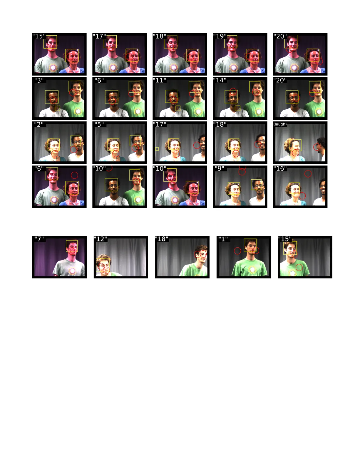
TRANSA CTIONS ON A UDIO, SPEECH, AND LANGU A GE PR OCESSING, V OL. 23, NO. 4, APRIL 2015 1 Co-Localization of Audio Sources in Images Using Binaural Features and Locally-Linear Re gression Antoine Deleforge ∗ Radu Horaud ∗ Y oav Y . Schechner ‡ Laurent Girin ∗ † ∗ INRIA Grenoble Rh ˆ one-Alpes, Montbonnot Saint-Martin, France † Uni v . Grenoble Alpes, GIPSA-Lab, France ‡ Dept. Electrical Eng., T echnion-Israel Inst. of T echnology , Haifa, Israel Abstract —This paper addresses the pr oblem of localizing audio sources using binaural measur ements. W e pr opose a super vised formulation that simultaneously localizes multiple sources at different locations. The approach is intrinsically efficient because, contrary to prior work, it r elies neither on source separation, nor on monaural segregation. The method starts with a training stage that establishes a locally-linear Gaussian regression model between the directional coordinates of all the sources and the auditory features extracted from binaural measurements. While fixed-length wide-spectrum sounds (white noise) are used f or training to reliably estimate the model parameters, we show that the testing (localization) can be extended to variable-length sparse-spectrum sounds (such as speech), thus enabling a wide range of realistic applications. Indeed, we demonstrate that the method can be used for audio-visual fusion, namely to map speech signals onto images and hence to spatially align the audio and visual modalities, thus enabling to discriminate between speaking and non-speaking faces. W e release a novel corpus of real-r oom recordings that allow quantitative evaluation of the co- localization method in the presence of one or two sound sources. Experiments demonstrate increased accuracy and speed relativ e to several state-of-the-art methods. Index T erms —Sound-source localization, binaural hearing, su- pervised learning, mixture model, regression, audio-visual fusion. I . I N T R O D U C T I O N W E address the problem of localizing one or sev eral sound sources from recordings gathered with two microphones plugged into the ears of an acoustic dummy head. This problem is of particular interest in the conte xt of a hu- manoid robot analyzing auditory scenes to better interact with its en vironment, e.g. [1]. The shape and morphology of such a binaural setup induce filtering ef fects, and hence discrepancies in both intensity-le vel and phase, at each frequency band, between the two microphone signals. These discrepancies are the interaur al level differ ence (ILD) and the interaural time differ ence (ITD) or equi v alently the interaur al phase dif fer ence (IPD). The ILD and IPD v alues across all frequencies are referred as binaural features . A. Deleforge, R. Horaud and L. Girin acknowledge support from the Eu- ropean Research Council through the ERC Advanced Grant VHIA #340113. Y . Y . Schechner is supported by the T echnion Autonomous Systems Program (T ASP) and Israel Science Foundation (ISF) Grant 1467/12. It was partially conducted in the Ollendorff Minerva Center, funded through the BMBF . YYS is a Landau Fellow supported by the T aub Foundation. For a single spatially-narrow emitter, the ILD and IPD depend on the emitter’ s position relative to the head, namely the 2D directional vector formed by azimuth and ele v ation. Binaural features hav e hence been used for single sound source localization (single-SSL), e .g. , [2], [3], [4], [5], [6], [7], [8], [9], [10], [11]. Matters are more complex when multiple sound sources, emitting from different directions, are simultaneously activ e. The sources mix at each microphone and the binaural features not only depend on the unknown emitting directions but also on the unkno wn emitted spectra. A common approximation assumes that any observed time- frequency (TF) point that has significant acoustic power is dominated by just a single source. This assumption, referred to as W -disjoint orthogonality (WDO) [12] simplifies the analysis: The binaural information at a TF point is simply related to the direction of a single source. WDO has been shown to be v alid to some extent in the case of mixtures of speech signals, though it may hav e limitations in dense cocktail party scenarios. State-of-the-art multiple-SSL techniques strongly rely on WDO to spatially gr oup binaural features, i.e. , to assign a giv en TF point to a single source [13], [14], [12], [15], [16], [17], [18], [19]. Some of these methods perform the grouping by selecting peaks in histograms of ITDs, accumulated over frequency channels [13], [12], [15], [17]. Other methods iterativ ely alternate between separation and localization [16], [19]. They require expectation-maximization (EM) inference at runtime, which is computationally intensiv e. The WDO assumption can also be combined with monaural segre gation. For e xample, in [14], [20], [18] azimuth is estimated from only those TF points at which a single source is thought to be dominant based on voiced and un v oiced speech cues. These monaural cues are then combined with a statistical model of ILD/ITD distribution that takes into account interfering sources, reverberation or background noise. The vast majority of the above-mentioned techniques limit single- and multiple-SSL to 1D localization, namely along the frontal azimuth direction and are based on a simplified sound propagation model. Moreov er , these methods attempt to extract localization information based on a physical model that must be somehow explicitly identified and inv erted, e.g . , the head- related transfer functions (HR TF) of the system. W e propose a method that directly localizes either a single 2 TRANSACTIONS ON A UDIO, SPEECH, AND LANGU A GE PR OCESSING, V OL. 23, NO. 4, APRIL 2015 or several sources simultaneously , on the following grounds: • it doesn’t rely on the WDO assumption, on source separation, or on monaural segregation; • it is based on learning a regression model that implicitly encodes the HR TF using training data; • it can use single-source data to train a multiple-source localization model; • it outperforms competing methods in terms of robustness, accuracy , and speed, and • it can be used to map sound sources onto images. A. Related W ork and Contributions T o overcome the need of a complex explicit sound propaga- tion model, a number of supervised approaches to SSL hav e been recently proposed. These methods use either artificial neural networks [2], manifold learning [8], [9] or regression [5], [9], [19], [22], [10], first to learn a mapping from binaural features to the (1D or 2D) direction of a single sour ce , and second to infer an unknown source direction from binaural ob- servations. These methods have the advantage that an explicit HR TF model is replaced by an implicit one, embedded in the parameters learned during the training stage. In general, the source used for training has a wide acoustic spectrum, e.g. , white noise (WN). A key feature common to all supervised- SSL methods is that their accuracy relies on the similarity between training and testing conditions, e .g. , setup, room, position in the room, etc., rather than on the similarity between a simplified model and real world conditions. In this paper we propose a supervised multiple-SSL method that requires neither source separation [16], [19] nor monaural segre gation [14], [20], [18]. Namely , we de vise a regression model that directly maps a binaural spectrogram onto the direction space (azimuth and elev ation) associated with a known number of simultaneously emitting sources M , i.e. , co-localization . This idea strongly contrasts with pre vious approaches in computational auditory scene analysis. Although strongly inspired by binaural hearing, it does not intend to mimic or emulate human perception but rather shows ho w new mathematical principles can be employed in practice for automated audition. The method starts with learning the parameters of a probabilistic locally-linear re gression model from associations between sound directions and binaural spec- trograms. Offline learning is followed by runtime testing : the learnt regression parameters are used to estimate a set of unknown source directions from an observed spectrogram. The latter is a time-series of high-dimensional binaural feature vectors (one vector at each time frame) that depend on source directions, source spectra, re verberations and ad- ditiv e noise. While emitted spectra, reverberations, and noise strongly v ary across both time and frequenc y , the directions are in variant, provided that the sources are static. The central idea in this paper is that the binaural features av ailable at TF points are dominated by the source dir ections , while they are perturbed by the temporal and spectral variations of monaural cues, noise and re verberations. There are hundreds of thousands of TF points in a one second spectrogram. Source- direction information can be gathered by aggregating all these observations. The above formulation leads to the problem of learning a high-dimensional to low-dimensional (high-to-lo w) regression, which is problematic for two reasons. Firstly , the large number of parameters that needs to be estimated in this case is pro- hibitiv e [23], [24]. Secondly , it is not clear how a regression, learnt with white-noise, can be used to locate natural sounds, e.g . , speech. Common sounds yield sparse spectrograms with many TF points having no source content. Methods such as [5], [8], [10] cannot handle natural sounds. A possible strategy could be to gather binaural features from relati vely long recordings, such that significant information becomes av ailable at each frequency band. In turn, it must be assumed that there is a single source emitting ov er a relativ ely long period of time, which is unrealistic in practice. For all these reasons we propose to adopt an in verse r e gression strategy [25]. W e devise a variant of the Gaussian locally-linear mapping (GLLiM) model, recently proposed [24]. W e learn a low-dimensional to high-dimensional (source- directions to binaural features) in v erse regression using a training dataset composed of associations between white- noise spectrograms and sound directions. Ref. [24] provides a closed-form expression for the forwar d or direct r e gression . In the context of multiple-SSL, this corresponds to the posterior distribution of source dir ections , conditioned by a binaural feature vector and giv en the learned parameters of the in v erse regression. In this paper we extend [24] to time series of high-dimensional v ectors with missing entries, i.e. , binaural spectrograms containing TF points with no source information. W e formally pro ve that the conditional posterior distribution that characterizes the spectrogram-to-source-directions map- ping is a Gaussian mixture model whose parameters (priors, means, and covariances) are expressed analytically in terms of the parameters of the lo w-to-high re gression. In practice we show that the proposed method robustly co-localizes sparse- spectrum sources that emit simultaneously , e.g., two speakers as illustrated in Fig. 1-Right. In v erse regression is also used in [9], [26] for single- SSL and in [19], [22] for simultaneous localization and separation . Howe ver , in addition to learning a regression, performing both localization and separation requires a time- consuming variational EM algorithm at runtime. Moreover , in [9], [19], [22] a binaural dummy head, mounted onto a pan-tilt mechanism, was used to collect datasets, i.e . , asso- ciations between motor positions and binaural spectrograms. The emitter was kept static at a unique position in all training and test experiments, while the dummy head was rotated onto itself. The method was hence limited to theoretical conclusions rather than practical applications. In this paper we introduce a novel and elegant way of gathering data with associated ground truth 1 . An audio-visual source , composed of a loud speaker and a visual marker , is manually held in front of the 1 The datasets are publicly a v ailable at https://team.inria.fr/perception/ the- av asm- dataset/. DELEFORGE et al. : CO-LOCALIZA TION OF AUDIO SOURCES IN IMAGES USING BINA URAL CUES AND LOCALL Y -LINEAR REGRESSION 3 Fig. 1. Left: Binaural recor dings and associated sound-source directions are simultaneously gathered with two microphones plugged into the ears of a dummy head and a camera placed under the head (only one of the two cameras is used in this work). The dummy head induces non-isotropic filtering effects responsible for 2D sound localization. Middle: T raining data are obtained as follows. A sound-direction-to-binaural-feature (low-to-high dimensional) regression is learned using an audio-visual target composed of a loud speaker and a visual marker . The loud-speaker that emits fixed-length full-spectrum sounds is moved in front of the dummy-head/camera device and for each loud-speaker location, both the emitted sound and the image location of the visual marker are recorded. The tiny red circles correspond to the 432 locations of the loud-speaker used for training. Right: Multiple sound-source localization . Based on the parameters of the trained regression, the sound directions (or equiv alently , image locations) are estimated from a variable-length sparse spectrogram (large red circles) in near real-time. The yellow square corresponds to the result of a face detector [21] which can only deal with frontal views. dummy head, and then mov ed from one position to the next. e.g . , Fig. 1. A camera is placed next to the dummy head. This setup allows to record synchronized auditory and visual signals. The horizontal and vertical positions of the loud- speaker marker in the image plane correspond to sound-source azimuth and elev ation. Moreover , if a talking person is present in front of the dummy-head/camera setup, his/her mouth can be easily located using f ace detection methods [21], [27]. Hence, accurate ground-truth source directions are av ailable in all cases and one can therefore quantify the performance of the proposed method. The remainder of the paper is organized as follows. Sec- tion II defines the concept of acoustic space and introduces the associated binaural features used in this study . Section III formulates multiple sound-source localization as a regression problem. Section IV presents the model used for mapping binaural features onto multiple sound source direction vectors. Section V extends this model to sparse binaural spectrogram inputs. Section VI presents obtained results for single source localization and source-pair co-localization. Section VII draws conclusions and directions for future work. I I . B I N AU R A L F E AT U R E S F O R L O C A L I Z AT I O N A. Acoustic Spaces Let us consider a binaural system, i.e . , two microphones plugged into the ears of a dummy head. This setup is used to record time series of binaur al featur e vectors in R D , i.e. , features capturing direction information associated with sev- eral sound sources. Section II-B details how such features are computed in practice. W e denote by D a set of sound-source directions in a listener-centered coordinate frame; namely D ⊂ R 2 is a set of (azimuth, ele vation) angles. W e denote by Y D ⊂ R D the subset of binaural feature vectors that can possibly be captured by the microphones when a single point sound-source m emits from x ( m ) ∈ D . In this article we restrict the analysis to static sources. W e refer to Y D as a simple-acoustic space of the binaural setup [22]. In this work we extend this concept to multiple static point sound-sources that emit simultaneously from M different directions. The set of sound directions is D M , the M − th Cartesian power of D . The multiple-acoustic space of the binaural system is the subset Y D M ⊂ R D of binaural feature vectors that can possibly be captured by the microphones when static sound sources emit from M directions in D M . W e represent an element of D M by a multiple-dir ection v ector x ∈ R L , where L = 2 M , e.g. , L = 4 in the case of tw o sources. Notice that in general the size of binaural feature vectors is much larger than the direction set dimension, namely D  L . Hence, the acoustic space Y D M forms an L − dimensional manifold embedded in R D . In this article, we sho w how the structure of this manifold can be learned in a supervised way , and used to build an efficient multiple ( M ) sound-source localizer . B. Binaural F eatur es W e consider a multi-direction vector x ∈ R L and we use the decomposition x = [ x (1) ; . . . ; x ( M ) ] , where x ( m ) ∈ R 2 denotes the direction of the m th source and [ . ; . ] is a notation for vertical concatenation. Let: s ( L ) = { s ( L ) f t } F,T f =1 ,t =1 ∈ C F × T s ( R ) = { s ( R ) f t } F,T f =1 ,t =1 ∈ C F × T (1) be complex-v alued spectrograms. These spectrograms are ob- tained from the left and right microphone signals using the short-time F ourier transform with F frequency bands and T time windows. Please see section VI for implementation details. W e consider two binaural spectrograms, namely the in- teraur al level differ ence (ILD) α = { α f t } F,T f =1 ,t =1 , and the 4 TRANSACTIONS ON A UDIO, SPEECH, AND LANGU A GE PR OCESSING, V OL. 23, NO. 4, APRIL 2015 interaur al phase differ ence (IPD), φ = { φ f t } F,T f =1 ,t =1 , which are defined as follows: α f t = 20 log | s ( R ) f t /s ( L ) f t |∈ R , (2) φ f t = exp  j arg( s ( R ) f t /s ( L ) f t )  ∈ C ≡ R 2 . (3) ILD and IPD cues, originally inspired by human hearing [28], have been thoroughly studied in computational binaural sound source localization [29]. These cues hav e proven their efficienc y in numerous practical implementations [14], [15], [16], [17], [18], [19] as opposed to, e.g. , the real and imaginary parts of the left-to-right spectrogram ratio, or monaural cues. Note that in our case, the phase difference is expressed in the complex space C (or equiv alently in R 2 ) to a void problems due to phase circularity . This representation allows two nearby phase values to be close in terms of their Euclidean distance, at the cost of a redundant representation. The regression model proposed in the next sections implicitly captures dependencies between observed features through a probabilistic model, and is therefore not affected by such redundancies. This method- ology was experimentally validated in [9]. The binaural spectr ogr am Y 0 = { y 0 dt } D,T d =1 ,t =1 is the con- catenation of the ILD and IPD spectrograms Y 0 = [ α ; φ ] ∈ R D × T , (4) where D = 3 F . Each frequency-time entry y 0 dt is referred to as a binaural feature . Let s ( m ) = { s ( m ) f t } F,T f =1 ,t =1 be the spectrogram emitted by the m th source. The acoustic wave propagating from a source to the microphones dif fracts around the dummy head. This propagation filters the signals, as expressed by the respec- tiv e left- and right comple x-valued HR TFs, h ( L ) and h ( R ) respectiv ely . The HR TFs depend on the sound-source direction and frequenc y . Interestingly , HR TFs not only depend on the azimuth of the sound source but also on its elev ation, due to the complex, asymmetrical shape of the head and pinna [30]. It is shown in [31] that HR TFs mainly depend on azimuth and elev ation while the distance has less impact in the far field (source distance > 1 . 8 meter). The relative influence of low- and high-frequency ILD and IPD cues on direction estimation was studied in [22]. By taking into account the HR TFs, the relationships between the emitted and perceived spectrograms write: s ( L ) f t = P M m =1 h ( L ) ( f , x ( m ) ) s ( m ) f t + g ( L ) f t , s ( R ) f t = P M m =1 h ( R ) ( f , x ( m ) ) s ( m ) f t + g ( R ) f t . (5) Here g ( L ) f t and g ( R ) f t denote some residual noise at left- and right-microphones at ( f , t ) , which may include self noise, background noise and/or low reverberations. Giv en the model (5), if none of the sources emits at ( f , t ) , i.e. , if s (1) f t = s (2) f t = . . . s ( M ) f t = 0 , then the corresponding binaural feature y 0 dt contains only noise, and hence it does not contain sound-source direction information. For this reason, such binaural features will be treated as missing . Missing binaural features are very common in natural sounds, such as speech. T o account for these missing features, we introduce a binary-valued matrix χ = { χ dt } D,T d =1 ,t =1 . W e use a threshold  on the power spectral densities, | s ( L ) f t | 2 and | s ( R ) f t | 2 , to estimate the entries of χ : χ dt = ( 1 if | s ( L ) f t | 2 + | s ( R ) f t | 2 ≥  0 otherwise. (6) The v alue of  is estimated by a veraging over time the measured noise power spectral density . Therefore, a binaural spectrogram: S = { Y 0 , χ } (7) is fully characterized by the binaural features Y 0 and the associated activity matrix χ . W e now consider the case where one or several sound sources emit at each frequency-time point ( f , t ) . The model (5) implies that the corresponding binaural features (4) depend on the sound-source directions, but also on the emitted sounds, and microphone noises. Ho we ver , while both the emitted sounds and the noise strongly vary across time and frequency , the sound-source directions are inv ariant, since the sources are static. With this in mind, a central postulate of this article is to consider that the binaural spectrogram entries { y 0 dt } D,T d =1 ,t =1 are dominated by sound-source directions and that they are perturbed by time-frequency v ariations of emitted sounds and of microphone noises. In other words, these variations are viewed as observation noise . This noise is expected to be very important, in particular for mixtures of natural sound sources. The proposed method will alleviate this issue by aggregating information over the entire binaural spectrogram S . This typically consists of hundreds of thousands of binaural features for a one second recording of speech sources. White-noise sources and associated binaural spectrograms are of crucial importance in our approach because the entire acoustic spectrum is being cov ered. In theory , white noise is a random signal with constant power spectral density ov er time and frequency . In practice, the recorded spectrogram of a white-noise source does not have null entries. Hence, χ = 1 D × T (all the entries are equal to 1 ), and a white- noise binaural spectrogram does not have missing values. Let S = { ( y 0 1 . . . y 0 t . . . y 0 T ) , 1 D × T } be a white-noise binaural spectrogram. T o reduce observation noise, we define the associated binaural feature vector as its temporal mean: y = 1 T T X t =1 y 0 t . (8) The set of binaural feature vectors y ∈ Y D M associated to sound source directions in x ∈ D M forms the multiple- acoustic space of our system. These vectors will be used to learn the relationship between input binaural signals and sound source directions. I I I . S U P E RV I S E D S O U N D L O C A L I Z AT I O N In the previous section we postulated that binaural features were dominated by sound-source direction information. In this section we describe a method that allows to learn a mapping DELEFORGE et al. : CO-LOCALIZA TION OF AUDIO SOURCES IN IMAGES USING BINA URAL CUES AND LOCALL Y -LINEAR REGRESSION 5 from these features to sound source directions using a regres- sion technique. More precisely , consider a training dataset of N binaural-feature-and-source-direction pairs { y n , x n } N n =1 , where y n ∈ Y D M ⊂ R D is a mean binaural feature v ector obtained from white noise signals (8), and x n ∈ D M ⊂ R L is the corresponding multiple-direction vector , i.e. , the azimuth and elev ation of M emitting sources. Notice that we hav e D  L . Once the regression parameters hav e been estimated, it is in principle possible to infer the unknown source direc- tions x from a spectrogram S = { Y 0 , χ } . Howe ver , there are two main difficulties when attempting to apply existing regression techniques to the problem of estimat- ing sound directions from a binaural spectrogram. Firstly , the input lies in a high-dimensional space, and it is well kno wn that high-dimensional regression is a difficult problem because of the very large number of model parameters to be estimated; this requires huge amounts of training data and may lead to ill-conditioned solv ers. Secondly , many natural sounds have sparse spectrograms and hence associated binaural spectro- grams often hav e a lot of missing entries. Nev ertheless, in practice the sound localizer should not be limited to white- noise signals. Therefore, the regression function at hand, once trained, must be extendable to predict an accurate output (sound directions) from any input signal, including a sparse binaural spectrogram. The proposed method bypasses the difficulties of high- dimensional to low-dimensional regression by considering the problem the other way around, i.e. , lo w-to-high, or in verse r e gression [25], [24]. W e assume that both the input and output are realizations of two random variables Y and X with joint probability distribution p ( Y , X ; θ ) , where θ denotes the model parameters. At training, the low-dimensional v ariable X plays the role of the re gressor , namely Y is a function of X possibly corrupted by noise through p ( Y | X ; θ ) . Hence, Y is assumed to lie on a low-dimensional manifold embedded in R D and parameterized by X . The small dimension of the regressor X implies a relatively small number of parameters to be estimated, i.e. , O [ L ( D + L )] . This facilitates the task of estimating the model parameters. Once θ has been estimated, we show that the computation of the forward conditional density p ( X | Y ; θ ) is tractable, and hence it may be used to predict the low-dimensional sound directions x associated with a high-dimensional mean binaural vector y . More detailed studies on the theoretical and experimental advantages of in v erse regression can be found in [25] and [24]. In practice we use a method referred to as pr obabilistic piecewise-af fine mapping [22] to train a lo w-dimensional to high-dimensional (directions-to-binaural-features) in verse r e- gr ession . This is an instance of the more general Gaussian locally-linear mapping (GLLiM) model [24], for which a Matlab implementation is publicly available. 2 The latter may be viewed as a generalization of mixture of e xperts [32] or of joint GMM [33]. W e then derive an analytic expression for the spectrogram-to-directions forwar d r e gr ession , namely the posterior distribution of sound directions conditioned by a 2 https://team.inria.fr/perception/gllim toolbox/. sparse spectrogram and gi ven the learned parameters of the in v erse regression. This distrib ution is a Gaussian mixture model whose parameters (priors, means, and co v ariances) ha ve analytic expressions in terms of the parameters of the inv erse regression. I V . P R O BA B I L I S T I C P I E C E W I S E - A FFI N E M A P P I N G This section presents the probabilistic piecewise-af fine map- ping model used for training. W e consider inv erse regression, namely fr om the low-dimensional space of sound directions to the high-dimensional space of white-noise spectr ograms . Any realization ( y , x ) of ( Y , X ) ∈ Y × D is such that y is the image of x by one affine transformation τ k among K , plus an error term. This is modeled by a missing variable Z such that Z = k if and only if Y is the image of X by τ k . The following decomposition of the joint probability distribution is used: p ( Y = y , X = x ; θ ) = K X k =1 p ( Y = y | X = x , Z = k ; θ ) · p ( X = x | Z = k ; θ ) · p ( Z = k ; θ ) . (9) The locally linear function that maps X onto Y is Y = K X k =1 I ( Z = k )( A k X + b k ) + E , (10) where I is the indicator function and Z is a hidden v ariable such that I ( Z = k ) = 1 if and only if Z = k , matrix A k ∈ R D × L and vector b k ∈ R D are the parameters of an af fine transformation τ k and E ∈ R D is a centered Gaussian error vector with diagonal co v ariance Σ = Diag ( σ 2 1 . . . σ 2 d . . . σ 2 D ) ∈ R D × D capturing both the observation noise in R D and the reconstruction error due to the local affine approximation. As already emphasized in [16], the well known correlation between ILD and IPD cues as well as the correlation of source spectra over frequencies does not contradict the assumption that Σ is diagonal, i.e. , the Gaussian noises corrupting binaural observations are independent. This assumption was proven to be reasonable in practice, e.g . [16], [22]. Consequently we hav e p ( Y = y | X = x , Z = k ) = N ( y ; A k x + b k , Σ ) . (11) T o make the transformations local, we associate each transfor- mation τ k to a region R k ∈ R L . These regions are modeled in a probabilistic way by assuming that X follows a mixture of K Gaussians defined by p ( X = x | Z = k ; θ ) = N ( x ; c k , Γ k ) , (12) with prior p ( Z = k ; θ ) = π k and with c k ∈ R L , Γ k ∈ R L × L , and P K k =1 π k = 1 . This may be viewed as a compact probabilistic way of partitioning the lo w-dimensional space into regions. Moreover , it allows to chart the high-dimensional space and hence to provide a piecewise affine partitioning of the data lying in this space. T o summarize, the model parameters are: θ = {{ c k , Γ k , π k , A k , b k } K k =1 , Σ } . (13) 6 TRANSACTIONS ON A UDIO, SPEECH, AND LANGU A GE PR OCESSING, V OL. 23, NO. 4, APRIL 2015 The parameter vector (13) can be estimated via an EM algorithm using a set of associated training data { y n , x n } N n =1 . The E-step ev aluates the posteriors r ( i ) kn = p ( Z n = k | x n , y n ; θ ( i − 1) ) (14) at iteration i . The M-step maximizes the expected complete- data log-likelihood with respect to parameters θ , giv en the observed data and the current parameters θ ( i ) , providing: θ ( i ) = argmax θ n E ( Z | X , Y , θ ( i − 1) ) [log p ( X , Y , Z | θ )] o . (15) Closed-form expressions for the E- and M-steps can be found in [22]. W e denote by e θ = θ ( ∞ ) the estimated parameter vector after con v ergence. The technique optimally partitions the low- and the high-dimensional spaces to minimize the reconstruction errors made by local affine transformations. It thereby captures the intrinsic structure of the acoustic space manifold Y D M . As a further justification for learning a low-dimensional to high-dimensional regression, let us consider the number of model parameters. W ith D = 1536 (the dimension of binaural feature vectors, see Section VI), L = 2 (single- source localization), and K = 10 (the number of affine transformations), there are approximately 45 , 000 parameters to be estimated (13), including the inv ersion of 2 × 2 full cov ariances { Γ k } k = K k =1 . If instead, a high-dimensional to low- dimensional regression is learned, the number of parameters is of the order of 10 8 and one must compute the in v erse of 1536 × 1536 full covariances, which would require a huge amount of training data. V . F R O M S PA R S E S P E C T RO G R A M S T O S O U N D D I R E C T I O N S W e no w consider the localization of natural sparse-spectrum sounds, e.g., speech mixtures. As already mentioned, a binau- ral spectrogram is described by S = { Y 0 , χ } , where Y 0 = { y 0 dt } D,T d =1 ,t =1 is a set of binaural features and χ = { χ dt } D,T d,t =1 is a binary-valued acti vity matrix. W e seek the posterior density of a set of sound directions, p ( x |S , e θ ) , conditioned by the observed spectrogram S and giv en the estimated model parameters e θ . W e state and prove the follo wing theorem which allows a full characterization of this density: Theorem 1. Under the assumption that all the feature vectors in S ar e emitted from fixed directions, the following posterior distribution is a Gaussian mixtur e model in R L , namely p ( x |S ; e θ ) = K X k =1 ν k N ( x ; µ k , V k ) . (16) whose parameter s { ν k , µ k , V k } k = K k =1 can be expr essed in closed-form with r espect to e θ and S , namely: µ k = V k  e Γ − 1 k e c k + D,T X d,t =1 χ dt e σ 2 d e a dk ( y 0 dt − e b dk )  , (17) V k =  e Γ − 1 k + D,T X d,t =1 χ dt e σ 2 d e a dk e a > dk  − 1 , (18) ν k ∝ e π k | V k | 1 2 | e Γ k | 1 2 exp  − 1 2  D,T X d,t =1 χ dt e σ 2 d ( y 0 dt − e b dk ) 2 + e c > k e Γ − 1 k e c k − µ > k V − 1 k µ k   , (19) wher e e a > dk ∈ R L is the d th r ow vector of e A k , ˜ b dk ∈ R is the d th entry of e b k and { ν k } K k =1 ar e normalized to sum to 1. The posterior expectation of (16) can then be used to predict sound directions: b x = E [ x |S ; e θ ] = K X k =1 ν k µ k . (20) W e refer to the resulting general sound sources localization method as supervised binaural mapping (SBM), or SBM- M where M is the number of sources. Documented Matlab code for this method is av ailable online 3 . Proof of theorem 1. By including the hidden variable Z (section IV) and using the sum rule, we obtain: p ( x |S ; e θ ) = K X k =1 p ( x |S , Z = k ; e θ ) p ( Z = k |S ; e θ ) . (21) Since the proposed model implies an af fine dependency be- tween the Gaussian v ariables X and Y gi ven Z , the term p ( x |S , Z = k ; e θ ) is a Gaussian distribution in x . In other words, for each k , there is a mean µ k ∈ R L and a co- variance matrix V k ∈ R L × L such that p ( x |S , Z = k ; e θ ) = N ( x ; µ k , V k ) . Notice that p ( Z = k |S ; e θ ) = ν k is not conditioned by x . W ith these notations, (21) leads directly to (16). W e no w de- tail the computation of the GMM parameters { µ k , V k , ν k } K k =1 . Using Bayes in version we have: p ( x |S , Z = k ; e θ ) = p ( S | x , Z = k ; e θ ) p ( x | Z = k ; e θ ) p ( S | Z = k ; e θ ) . (22) Since we already assumed that the measurement noise has a diagonal cov ariance Σ , the observ ations in S are condition- ally independent giv en Z and x . Therefore, by omitting the denominator of (22) which does not depend on x , it follows that p ( x |S , Z = k ; e θ ) is proportional to p ( x | Z = k ; e θ ) Q D,T d =1 ,t =1 p ( y 0 dt | x , Z = k ; e θ ) χ dt = N ( x ; e c k , e Γ k ) Q D,T d =1 ,t =1 N ( y 0 dt | e a > dk x + e b dk , e σ 2 d ) χ dt = C | e Γ k | 1 2 exp  − 1 2 ( A + B )  , (23) 3 https://team.inria.fr/perception/research/binaural- ssl/ DELEFORGE et al. : CO-LOCALIZA TION OF AUDIO SOURCES IN IMAGES USING BINA URAL CUES AND LOCALL Y -LINEAR REGRESSION 7 where A = P D,T d =1 ,t =1 χ dt e σ 2 d ( y 0 dt − e a > dk x − e b dk ) 2 (24) B = ( x − e c k ) > e Γ − 1 k ( x − e c k ) , (25) and C is a constant that depends neither on x nor on k . Since p ( x |S , Z = k ; e θ ) is a normal distribution in x with mean µ k and covariance V k , we can write: A + B = ( x − µ k ) > V − 1 k ( x − µ k ) . (26) By developing the right-hand side of (26) and by identification with the expressions of A (24) and B (25), we obtain the formulae (17) and (18) for µ k and V k respectiv ely . Using Bayes in version, one can observe that the mixture’ s priors ν k = p ( Z = k |S ; e θ ) are proportional to e π k p ( S | Z = k ; e θ ) . Unfortunately , we cannot directly decompose p ( S | Z = k ; e θ ) into a product over ( d, t ) , as pre viously done with p ( S | x , Z = k ; e θ ) . Indeed, while it is assumed that the frequency-time points of the observed spectrogram S are independent given x and Z , this is not true for the same observations given only Z . Howe ver , we can use (22) to obtain p ( S | Z = k ; e θ ) = p ( S | x , Z = k ; e θ ) p ( x | Z = k ; e θ ) p ( x |S , Z = k ; e θ ) . (27) The numerator is gi ven by (23) and the denominator is the normal distribution N ( x ; µ k , V k ) . After simplifying the terms in x , we obtain the desired expression (19) for ν k .  V I . E X P E R I M E N T S A N D R E S U LT S In this section, the proposed binaural localization method is ev aluated with one source ( M = 1 , L = 2 ) as well as with two sources ( M = 2 , L = 4 ). W e gathered several datasets using the following experimental setup. A camera is rigidly attached next to a binaural Senheiser MKE 2002 acoustic dummy head, e.g., Fig. 1-left and Fig. 2-left. W e used two cameras, one with a resolution of 640 × 480 pixels and a horizontal × vertical field of view of 28 ◦ × 21 ◦ , and another one with a resolution of 1600 × 1200 pixels and a horizontal × vertical field of view of 62 ◦ × 48 ◦ . W ith these two cameras, a horizontal field of view of 1 ◦ corresponds to 23 pix els and 26 pix els, respecti vely . Assuming a linear relationship, pixel measurement can be con v eniently con verted into degrees. The dummy-head-and- camera recording setup is placed approximately in the middle of a room whose rev erberation time is T 60 ≈ 300 ms. Low background noise ( < 28 dBA) due to a computer f an was present as well. All the recordings (training and testing) were performed in the same room. In general, we used the same room location for training and for testing. In order to quantify the robustness of the method with respect to room locations, we carried out experiments in which we used one room location for training and another room location for testing, i.e. , Fig. 2-right. The training data were obtained from a loudspeaker . The test data were obtained from a loudspeaker , and from people speaking in front of the recording device. All the training and test datasets hav e associated ground-truth obtained as follows. A visual pattern, which can be easily detected and precisely located in an image, was placed on the loudspeaker (Fig. 1- middle). This setup allows us to associate a 2D pixel location with each emitted sound. Moreo v er , we used the Zhu-Ramanan face detection and localization method [27] that enables ac- curate localization of facial landmarks, such as the mouth, in the image plane (errors made by the mouth localization method were manually corrected). Therefore, pixel positions, or equiv alently sound directions, are always av ailable with the recorded sounds. T o ev aluate SSL performance, we define the gr ound-truth-to-estimate angle (GTEA). This corresponds to the distance between the expected sound source location (loud- speaker or mouth) and the estimated one, conv erted to degrees. This allows quantitative ev aluation of the proposed method’ s accuracy , and comparison with other methods using the same datasets. Binaural feature v ectors are obtained using the short-time Fourier transform with a 64ms Hann window and 56ms ov erlap, yielding T = 125 windo ws per second. Each time window therefore contains 1024 samples, transformed into F = 512 complex Fourier coefficients covering 0Hz–8kHz. W e considered the following binaural feature vectors: ILD only , namely (2) with D = F = 512 , IPD only , namely (3) with D = 2 F = 1024 , and concatenated ILD-IPD referred to as ILPD, namely (4) with D = 3 F = 1536 . T raining data were gathered by manually placing the loud- speaker at 18 × 24 = 432 grid positions lying in the camera’ s field of view and in a plane which is roughly parallel with the image plane, two meters in front of the setup (Fig. 1- middle). One-second long white-noise (WN) signals and the corresponding image positions were synchronously recorded. The training data are referred to as the loudspeaker -WN data. This dataset can straightforwardly be used to train a single- source localizer ( M = 1 ). Importantly , training the multiple- source co-localization does not require any additional data. Indeed, the single source training dataset can also be used to generate a two-source training dataset ( M = 2 ), by randomly selecting source pairs with their image-plane locations and by mixing up the two binaural recordings. Similarly , we gathered a test dataset by placing the loud- speaker at 9 × 12 = 108 positions. At each position, the loudspeaker emitted a 1 to 5 seconds random utterance from the TIMIT dataset [34]. T wo-source mixtures were obtained by summing up two binaural recordings from these test data. As was the case with the training data, the 2D directions of the emitted sounds are a v ailable as well, thus provid- ing the ground-truth. These test data are referred to as the loudspeaker -TIMIT data. A more realistic test dataset aiming at reproducing different natural auditory scenes was gathered with one and two live speakers in front of the dummy head and camera, at a distance varying between 1.8 and 2.2 meters. W e tested the following scenarios: • Moving-speaker scenario (narrow field-of-view camera lens). A single person counts in English from 1 to 20. The person is approximativ ely still (small head mov ements are unav oidable) while she/he pronounces an isolated speech 8 TRANSACTIONS ON A UDIO, SPEECH, AND LANGU A GE PR OCESSING, V OL. 23, NO. 4, APRIL 2015 Fig. 2. Left: A typical recording session. The two microphones plugged into the ears of the dummy head are the only ones used in this paper , although the head is equipped with four microphones. Right: T op view of the recording room. The robustness of the method with respect to room changes is validated by using different locations for training with white noise emitted by a loudspeaker (green zone #1) and for testing with human speakers (yellow zone #2). utterance, whereas she/he is allowed to wander around in between two consecuti ve utterances • Speaking-turn scenario (wide field-of-vie w camera lens). T wo people take speech turns (they count from 1 to 20) with no temporal overlap, in different languages (English, Greek, Amharic). They are allowed to move between two consecutiv e utterances. • T wo-speaker scenario (narro w field-of-view camera lens). T wo people count simultaneously from 1 to 20 in different languages (English, French, Amharic) while they remain in a quasi-static position through the entire recording (see the paragraph below). These li v e test data are referred to as the person-li ve dataset. All the training and test datasets, namely loudspeaker -WN , loudspeaker -TIMIT , and person-live are publicly av ailable 4 . Notice that ground-truth 2D source directions are available with all these data, hence they can be used indifferently for training and for testing. The li ve recordings are particularly challenging for many reasons. The sounds emitted by a live speaker have a large variability in terms of direction of emis- sion ( ± 30 ◦ ), distance to the binaural dummy head ( ± 50 cm), loudness, spectrogram sparsity , etc. Moreov er , the people hav e inherent head motions during the recordings which is likely to add perturbations. Therefore, there is an important discrepancy between the training data, carefully recorded with a loudspeaker emitting white-noise, and these test data. In all the person-live scenarios, a fixed-length analysis segment is slid along the time axis and aligned with each video frame (segments are generally o verlapping). The proposed supervised binaural mapping methods, namely SBM-1 and SBM-2 (20), are applied to the segments that yield a sufficient acoustic lev el. The sound-source localization results obtained for each segment are then represented in their corresponding video frame. 4 https://team.inria.fr/perception/the- av asm- dataset/ A. Single-Source Localization W e first e v aluate our supervised binaural mapping method in the single source case ( M = 1 , L = 2 ), i.e. , SBM-1. Training was done with N = 432 binaural feature vectors associated to single source directions, using K = 32 (13.5 points per affine transformation) and white noise recordings made with the 28 ◦ × 21 ◦ field of view camera. The ov erall training computa- tion took around 5.3 seconds using Matlab and a standard PC. W e compared our method with the baseline sound source lo- calization method PHA T -histogram, here abbreviated as PHA T [35], [13]. PHA T -histogram estimates the time differ ence of arrival (TDO A) between microphones by pooling o ver time generalized cross-correlation peaks, thus obtaining a pseudo probability distrib ution 5 . In all experiments, the same sampling frequency (16kHz) and the same sound length is used with PHA T and with our method. A linear regression was trained to map TDOA values obtained with PHA T , onto the horizontal image axis using loudspeaker-WN training data 6 . Notice that PHA T , as well as all binaural TDOA-based localization methods, cannot estimate the vertical position/direction. The few existing 2D sound source localization methods in the literature, e.g., [4], could not be used for comparison ([4] relies on artificial ears with a spiral shape). 1) Loudspeaker Data: The single-source localization re- sults using the loudspeaker-TIMIT dataset are summarized in T able-I. The best results are obtained using the proposed method SBM-1 and ILPD spectrograms, i.e. , (4). The largest GTEA is then 3 . 94 ◦ which corresponds to 90 pixels. The largest GTEA with PHA T is 9 ◦ , and PHA T yields 14 GTEA values (out of 108 tests) which are larger than 5 ◦ . The proposed method outperforms PHA T , both in terms of the 5 W e used the PHA T -histogram implementation of Michael Mandel, av ail- able at http://blog.mr-pc.or g/2011/09/14/messl-code-online/. This TDOA esti- mator has a sub-sample accuracy , allowing for non-integer sample delays. 6 A linear dependency between TDOA values obtained with PHA T using a single white-noise source and its horizontal pixel position was observed in practice. DELEFORGE et al. : CO-LOCALIZA TION OF AUDIO SOURCES IN IMAGES USING BINA URAL CUES AND LOCALL Y -LINEAR REGRESSION 9 av erage error of the inliers and in the percentage of outliers, while localizing the source in 2D. The av erage CPU time of our method implemented in MA TLAB, using ILPD spectrograms, is of 0.23s for one second utterances, which is comparable to PHA T’ s CPU time. W e measured the ef fect of introducing the binary activity matrix χ (see Section II-B and eq. (16)-19)). For the single- source case, taking the entire spectrogram into account instead increased the localization errors of our method by 7% in av erage. T ABLE I S I NG L E - SO U R C E L O CA L I Z A T I O N R E S ULT S W I T H T H E L O UD S P E AK E R - TI M I T T E S T DAT A , U S I N G T H E P RO P O SE D M E TH O D ( W IT H I L D -, I P D -, A N D I L P D - S P E C TR OG R A M S ) A N D P H A T. T H E A V E R AG E A N D S TA ND A RD D E V IAT IO N ( A V G ± S T D ) O F T H E G T E A A R E E S TI M A T ED O VE R 1 0 8 L O C A LI Z A T I ON S . T H E F O U RT H C O LU M N P ROV I D ES T H E P E RC E N T AG E O F G T E A G R E A T ER T H A N 5 ◦ . Method Azimuth ( ◦ ) Elev ation ( ◦ ) > 5 ◦ (%) CPU time (s) ILPD 0.96 ± 0.73 1.07 ± 0.92 0.0 0.23 ILD 1.20 ± 0.99 1.09 ± 1.45 1.9 0.08 IPD 1.05 ± 0.90 1.46 ± 1.70 5.6 0.15 PHA T 2.80 ± 2.25 - 14 0.37 Fig. 3 shows the influence of the free parameters of training on the proposed method, namely the number of Gaussian component K and the size of the training set N . As can be seen in Fig. 3-left, K can be chosen based on a compromise between computational time and localization accuracy . Note that in this example, results do not improv e much for initial K values larger than 10 . This is notably because too high values of K lead to degenerate covariance matrices in classes where there are too fe w samples. Such classes are simply remov ed along the execution of the algorithms, thus reducing the final value of K . As can be seen in Fig. 3-right, the number of training points N has a notable influence on the localization accuracy . This is because the larger the N , the larger the angular resolution of the training set. Ho we ver , using N = 100 instead of N = 432 increases the av erage GTEA by less than 1 ◦ . This suggests that a less dense grid of points could be used for simple, practical training. While manually recording 432 positions took 22 minutes, a training set of 100 positions can be recorded in 5 minutes. 2) P erson-Live Data: T o illustrate the effecti veness of the proposed framework in real world conditions, we applied the SBM-1 method to the moving-speaker scenario of the person- live dataset. A 720 ms sliding segment was used, allowing to obtain a sound source direction for each video frame with a sufficient acoustic level. Fig. 4 shows an example frame for each pronounced number . Note that in this experiment as well as in all the person-li ve experiments, the example frames are manually selected so that the corresponding anal- ysis segments are roughly centered on the uttered numbers. Segments containing only a small part of a utterance, two consecutiv e utterances, or a high amount of late rev erberations generally yielded unpredictable localization results. This can be observed in the online videos 7 . This could be addressed by 7 https://team.inria.fr/perception/research/binaural- ssl/ using a more advanced speech activity detector to adjust the size and position of the analysis segment, as well as a tracker that takes into account past information. The estimated location of the sound-source is shown with a red circle. For comparison, Fig. 4 also shows face local- ization estimates obtained with an efficient implementation of the V iola-Jones face detector [21]. This implementation has CPU performance comparable to our method while the more precise Zhu-Ramanan face detector [27] used for ground-truth annotation is two orders of magnitude slower . Our method localizes the 20 uttered numbers, with an average GTEA and standard deviation of 1 . 8 ◦ ± 1 . 6 ◦ in azimuth and 1 . 6 ◦ ± 1 . 4 ◦ in elev ation. The largest GTEA (number “10”), is of 6 . 6 ◦ in azimuth and 3 . 4 ◦ in elev ation. For comparison, the av erage azimuth localization error with PHA T -histogram is 2 . 7 ◦ ± 1 . 9 ◦ on the same data, with a maximum error of 6 . 6 ◦ . Interestingly , the V iola-Jones method [21] correctly detects and localizes the face in 16 out of 20 tests, b ut it fails to detect the face for “8”, “9”, “17” and “18”. This is because the face is only partially visible in the camera field of view , or has changing gaze directions. Moreover , it features se veral false detections (“1”, “5”, “8”, “10”). These examples clearly sho w that our method may well be viewed as complementary to visual face detection and localization: it localizes a speaking face ev en when the latter is only partially visible and it discriminates between speaking and non-speaking faces. 3) Robustness to Locations in the Room: The proposed method trains a binaural system in a reverberant room and at a specific room location. In such an echoic en vironment, the learned parameters are therefore lik ely to capture the HR TF as well as the room impulse response. W e remind that the method essentially relies on the similarity between training and testing conditions, rather than on the similarity between a simplified acoustic model and real world conditions. In previous experiments, the training and testing positions were almost the same. The objectiv e of this experiment is 0 10 20 30 1.5 2 2.5 3 3.5 4 Mean SBM − 1 Localization Error (degrees) 0 10 20 30 0 0.1 0.2 0.3 0.4 Computational time (seconds) Number of Components K 100 200 300 400 1.8 2 2.2 2.4 2.6 2.8 3 Training Set Size N Mean SBM − 1 Localization Error (degrees) Fig. 3. Left: Influence of K on the mean GTEA and localization time of a 1 second speech source using the proposed supervised binaural mapping method ( M = 1 , N = 432 ). Right: Influence of N on the mean GTEA of a 1 second speech source ( K = 32 ). 10 TRANSA CTIONS ON A UDIO, SPEECH, AND LANGUA GE PROCESSING, VOL. 23, NO. 4, APRIL 2015 Fig. 4. The moving-speaker scenario. The person is static while he pronounces a number (written in white) and he mo ves between tw o numbers. The red circles show the position found with our method. The yello w squares correspond to faces detected with [21]. The full video is a vailable at https://team.inria.fr/perception/research/binaural-ssl/. Fig. 5. Examples of localization results with a wider field-of-view camera ( 62 ◦ × 48 ◦ ) in a location that is different than the location used for training. Notice that overall, the method is relatively robust to changes in the room impulse response. The red circles show the position found with our method. The yellow squares show the results of the V iola-Jones face detector[21]. While the accuracy in azimuth is not significantly affected, the accuracy in elevation is significantly degraded. The full video is available at https://team.inria.fr/perception/research/binaural-ssl/. to verify whether the proposed method yields some degree of robustness to changes in room impulse responses, e.g. , the training and testing occur at two different positions in the room. Moreov er , for these experiments we used a camera with a larger field of view , namely 62 ◦ × 48 ◦ . Figure 2-right shows a top vie w of the recording room with a training zone and a test zone. The microphone-to-emitter distance vary from 2 m (training) to approximately 1.8 m (testing). The SBM- 1 method is applied to the speaking-turn scenario for testing. The procedure already described abov e is used to train the model, to localize sounds online and to select example frames. This time, a 1000 ms analysis segment is used, as it improves the overall performance. Figure 5 shows some of the results obtained with human speakers using single-source training. Out of 23 uttered num- bers, the average azimuth error is 4 . 7 ◦ ± 2 . 7 ◦ with a maximum error of 9 . 9 ◦ . The average elev ation error is 7 . 3 ◦ ± 4 . 6 ◦ ex- cluding three outliers having an error larger than 15 ◦ degrees, e.g . , Fig. 5, second row , third column. Note that the increased camera field of vie w decreased the angular resolution of the training set by a factor 2 . 2 (1 point ev ery 2 . 5 ◦ in azimuth and elev ation). This decreased resolution yields a slight increase DELEFORGE et al. : CO-LOCALIZA TION OF AUDIO SOURCES IN IMAGES USING BINA URAL CUES AND LOCALL Y -LINEAR REGRESSION 11 in azimuth localization error , consistently with observations in Fig. 3-right. But overall, the azimuth accuracy does not seem to be significantly af fected by changes of microphone locations in the room. On the other hand, the elev ation accuracy is significantly decreased, with errors 4.6 times larger , and 8 . 7% of outliers instead of none. This suggests that making elev ation estimation more robust would require combining training data from different real and/or simulated rooms. For comparison, the baseline algorithm PHA T is used on the same test data. As in previous experiments, a linear dependency between TDO A values estimated by PHA T and the horizontal image axis was observed. For fairness, this dependency was modeled by learning a linear regression model using the white-noise recordings from the training zone (Figure 2-right). The av erage azimuth error of PHA T ov er 23 uttered numbers is 5 . 4 ◦ ± 2 . 9 ◦ with a maximum error of 11 . 8 ◦ . In this realistic scenario with different training and testing locations, the proposed approach still performs better and more robustly than the baseline PHA T -histogram method in azimuth only , while it estimates the elev ation as well. B. T wo-Source Localization In this section, we present a key result of the proposed framew ork: it successfully maps binaural features to the direction-pair of two simultaneous sound sources without relying on sound source separation. This is solely achie ved based on supervised learning. This instance corresponds to the case M = 2 , L = 4 , and is thus referred to as SBM-2 . Training was based on N = 20 , 000 binaural feature vectors associated to source-pair directions, using K = 100 (200 points per af fine transformation). The overall training took 54 minutes using Matlab and a standard PC. W e compared SBM-2 to three other multiple SSL methods: PHA T -histogram [13], MESSL [16] and VESSL [19]. PHA T - histogram can be used to localize more than one source by selecting M peaks in the histograms. MESSL is an EM- based algorithm which iterativ ely estimates a binary mask and a TDOA for each source. The version of MESSL used here is initialized by PHA T -histogram and includes a garbage component as well as ILD priors to better account for rever - berations. As in pre vious section, a linear regressor w as trained to map PHA T’ s and MESSL ’ s TDO A estimates to horizontal pixel coordinates. The supervised method VESSL may be viewed as an extension of SBM-1 to multiple sound source separation and localization. Similarly to MESSL, VESSL uses a variational EM procedure to iteratively estimate a binary mask and a 2D direction for each source. It was trained using the single-source loudspeaker-WN dataset ( N 0 = 432 ILPD feature vectors) and K 0 = 32 affine component. This method, as well as PHA T -histogram and MESSL, strongly rely on the assumption that emitting sources are sparse, so that a single source dominates each time-frequency bin (WDO). This is not the case of SBM-2, since it is trained with strongly ov erlapping white-noise mixtures. 1) Loudspeaker Data: The methods were first tested using the loudspeaker datasets. W e tested 1000 source-pair mixtures of the following types: white-noise + white-noise (WN+WN), white-noise + speech (WN+S) and speech + speech (S+S). Each mixture was cut to last 1 second. The av erage amplitude ratio of source-pairs was 0 ± 0 . 5 dB in all mixtures. The maximum azimuth and ele v ation distances between two test sources was 20 ◦ , and the minimal distance was 1 . 5 ◦ . T able II displays errors in azimuthal/horizontal and ele- vation/v ertical localization, in degrees. For WN+S mixtures, localization errors for white-noise sources (WN) and speech (S) sources are shown separately . Generally , the SBM-2 out- performs PHA T , MESSL, and VESSL in terms of accuracy , while localizing sources in 2D. Again, best results were ob- tained using ILPD features. SBM-2 performs best in WN+WN mixtures. This is expected because it corresponds to mixtures used for training the algorithm. Howe ver , the proposed method also yields good results in speech localization, e ven in the very challenging WN+S mixtures, despite an average speech- to-noise ratio of 0 ± 0 . 5 dB. It also yields good results for S+S mixtures, e v en though in this case both sources are sparse. This shows that aggregating a large number of binaural features in the time-frequency plane is a successful strategy to overcome the high variability of emitted signals which affects binaural features. Moreov er , introducing the binary activity matrix χ reduced the av erage localization errors of our method by 25% for white-noise sources and 15% for speech sources. Although both SBM-2 and VESSL are based on supervised learning, our method yields significantly better results than the VESSL. This demonstrates the prominent advantage of relaxing the WDO assumption for multiple sound-source localization. The proposed method reduces the localization error by 60% with respect to the second best method VESSL in a two-speak er scenario. Such a gain can be critical to correctly identify speaking people in a dense cocktail party scenario, e.g , two people talking one meter from each other, 2 meters away from the setup. The fact that VESSL, MESSL and PHA T perform poorly in WN+WN mixtures is expected, because then the WDO assumption is strongly violated. In WN+S mixtures, they sho w better performance in localizing the white noise sound source than the speech source. This can be explained by the sparsity of the speech signal. This implies that most binaural cues in the time-frequency plane are generated by the white noise source only . These cues are correctly clustered together assuming WDO, and can then be accurately mapped to the correct source direction. In the particular case of WN localization in WN+S mixtures, the average azimuth error of VESSL is e ven slightly lo wer than that of SBM-2. Possibly , this is because VESSL uses 32 affine components and a single source training ( L = 2 ), while SBM-2 uses 100 affine components and a two sources training ( L = 4 ). The av erage angular area per source cov ered by af fine transformations is thus higher in VESSL ( 4 . 3 ◦ × 4 . 3 ◦ on an a verage) than in SBM-2 ( 7 . 7 ◦ × 7 . 7 ◦ on an average). Computational times of PHA T , MESSL, VESSL ( K 0 = 32 ) and SBM-2.ILPD ( K = 100 ) for a one second test mixture 12 TRANSA CTIONS ON A UDIO, SPEECH, AND LANGUA GE PROCESSING, VOL. 23, NO. 4, APRIL 2015 T ABLE II S O UR C E PA I R L O CA L I Z A T I O N R E S ULT S F O R D I FF E RE N T M I X T UR E T Y PE S U S I NG S B M -2 A N D D I FF E RE N T M E T H OD S . E R RO R A V E R AG E S A N D S TAN D AR D D E VI ATI O N S ( A V G ± S T D ) A R E S H OW E D I N D E G RE E S . A VG S A N D S T DS A R E O N L Y C A LC U L A TE D OV E R I N L Y I NG E S T IM ATE S . E S T I MAT ES A R E C O NS I D E RE D O U TL I E R S I F T H E I R D I STA N CE T O G RO U N D - T RU T H I S M O R E T H AN 15 ◦ . P E R C EN TAG E S O F O U T L IE R S A R E G I V E N I N C O L U MN S “ O UT ” . Mixture WN+WN WN+S (WN) WN+S (S) S+S Method azimuth ele vation out azimuth elevation out azimuth ele v ation out azimuth ele vation out SBM-2.ILPD 0.76 ± 0.84 0.99 ± 1.11 0.0 0.83 ± 1.18 0.69 ± 1.00 0.0 3.22 ± 3.11 3.60 ± 3.21 9.1 1.39 ± 1.40 1.99 ± 2.30 0.4 SBM-2.ILD 1.03 ± 1.51 1.08 ± 1.55 0.1 1.19 ± 1.89 1.15 ± 1.74 0.7 3.28 ± 3.03 3.74 ± 3.31 7.8 2.19 ± 2.69 2.48 ± 2.85 3.1 SBM-2.IPD 1.14 ± 1.28 1.47 ± 1.94 0.0 1.01 ± 1.28 0.88 ± 1.33 0.3 3.71 ± 3.32 4.09 ± 3.36 9.1 2.00 ± 2.08 2.58 ± 2.73 1.3 VESSL[19] 3.20 ± 3.47 3.51 ± 3.65 17 0.62 ± 1.13 0.73 ± 1.10 1.6 5.90 ± 3.91 5.35 ± 3.84 35 3.47 ± 3.41 3.69 ± 3.57 11 MESSL[16] 4.11 ± 3.88 − 24 2.85 ± 3.99 − 25 6.66 ± 4.26 − 28 4.05 ± 3.90 − 19 PHA T[13] 4.01 ± 3.89 − 24 2.86 ± 3.98 − 25 6.53 ± 4.26 − 28 4.09 ± 3.85 − 18 were respectiv ely 0 . 27 ± 0 . 01 s , 10 . 4 ± 0 . 1 s, 46 . 7 ± 1 . 2 s and 2 . 2 ± 0 . 1 s using MA TLAB and a standard PC. With proper optimization, SBM-2 is therefore suitable for real-time applications. This is not the case for MESSL and VESSL, due to their iterativ e nature. While the of fline training of SBM methods requires a computationally costly EM procedure, the localization is very fast using the closed-form expression (20). As in pre vious section, we tested the influence of the number of affine components K and training set size N on SBM-2 performance. By Fig. 6-left, K can again be tuned based on a trade-off between computation time and accuracy . Choosing K = 20 brings do wn the co-localization time of a 1 second mixture to 0.42 seconds, while increasing the localization error by only 6 . 5% relati ve to K = 100 . Fig. 6-right shows that localization error increases when N decreases. Howe v er , using N = 5 , 000 increases the mean localization error by only 3 . 2% relativ e to N = 20 , 000 . Again, this suggests that a less dense grid of points can be used for faster training (a training set of 100 positions can be recorded in 5 minutes and allows N = 5 , 050 source pairs). W e further examined the behavior of SBM-2 in two extreme cases. First, we tested the approach on mixtures of two equal sound sources, i.e. , recordings of two loudspeakers emitting the same TIMIT utterance at the same time from two differ - ent directions. In that case, the two sources are completely ov erlapping. Over the 19 test mixtures (38 localization tasks), 0 50 100 1.5 2 2.5 3 3.5 4 Mean SBM − 2 Localization Error (degrees) 0 50 100 0 1 2 3 Computational time (seconds) Number of Components K 0 10000 20000 1.8 1.9 2 2.1 2.2 2.3 Training Set Size N Mean SBM − 2 Localization Error (degrees) Fig. 6. Left: Influence of K on the mean GTEA and localization time of a 1 second S+S mixture using the proposed supervised binaural mapping method ( M = 2 , N = 20 , 000 ). Right: Influence of N on the mean GTEA of a 1 second S+S mixture ( K = 100 ). SBM-2 yielded an av erage error of 1 . 5 ◦ in azimuth, 2 . 0 ◦ in elev ation, and only one error larger that 10 ◦ . This is similar to results obtained on S+S mixtures with distinct speech signals (T able II). On the other hand, the 3 other methods [13], [16], [19] failed to localize at least one of the two sources (more than 10 ◦ error) in more than half of these tests. This result may seem counter-intuiti ve at first glance. Indeed, a human listener would probably confuse the two identical sources with a single source located somewhere in between the two sources. Howe ver , it is in fact unlikely that the set of D = 1536 frequency-dependent binaural features generated by the two sources matches exactly the set of binaural features generated by a single source at a dif ferent location. This result stresses that the proposed co-localization method outperforms traditional WDO-based approaches in heavily ov erlapping mixtures. Second, we tested the approach on 100 non-overlapping mixtures, i.e. , tw o consecuti ve 500ms speech segments emitted from different directions. Results obtained with all 4 methods were similar to those obtained for S+S mixtures in T able II. Although ILD and IPD cues depend on the relativ e spectra of emitting sources (5), these last experiments show that SBM-2 is quite robust to v arious type of overlap in mixtures. This is because a lar ge number of binaural features are gathered ov er the TF plane, thus alleviating perturbations due to v arying source spectra (Section II-B). 2) P erson-Live Data: SBM-2 was also tested on the more realistic two-speaker scenarios. A 1200ms sliding analysis temporal segment was used in order to estimate the two speaker positions. Smaller analysis segments de graded the results. This shows the necessity of gathering enough binaural features for the SBM-2 method to work. Fig. 7 shows some frames of the video generated from this test. The sound source positions estimated by SBM-2 are shown by a red circle in the corresponding video frame. Three couples of participants were recorded, totaling 124 numbers pronounced. In all experiments, SBM-2 corr ectly localized at least one of the two simultaneous sources in both azimuth and elev ation, where correctly means less than 4 ◦ error (this approximately correspond to the diameter of a face in the image space). Out of the 124 uttered numbers, 92 (74.1 % ) were correctly localized in both azimuth and elev ation. Out of the remaining 32 mistaken localizations, 18 had a correct azimuth estimation ( e.g . , Fig. 7 last row , column 1 and 2), 4 were mistaken for the other source ( e.g. , Fig. 7 last row , column 3) and only 10 ( 8% ) were incorrectly localized in both azimuth and elev ation ( e.g . , Fig. 7 last row , column 4 and 5). Results obtained with DELEFORGE et al. : CO-LOCALIZA TION OF AUDIO SOURCES IN IMAGES USING BINA URAL CUES AND LOCALL Y -LINEAR REGRESSION 13 Fig. 7. T wo subjects count from 1 to 20 (white numbers) in different languages, with a normal voice loudness, from a fixed position. The red circles show the position found with our method. The yellow squares show the results of the V iola-Jones face detector[21]. The first 3 rows sho w examples of successful localization results, the last row shows examples of typical localization errors. Full videos av ailable at https://team.inria.fr/perception/research/binaural-ssl/. (a) (b) (c) (d) (e) Fig. 8. Examples of results obtained with SBM-2 (red circles) on a single source scenario. The yellow squares are the faces detected with [21]. The full video is av ailable at https://team.inria.fr/perception/research/binaural-ssl/. the V iola-Jones face detection algorithm [21] are shown with a yello w square. The face-detector yielded a few erroneous results due to partial occlusions and false detections. Finally , Fig. 8 shows some examples of the output of SBM- 2 on a single source scenario. For 8 out of 20 numbers, the algorithm returned two source positions near the actual source, e.g . Fig. 8(a)(b)(c). This is because the two-source training set also includes mixtures of nearby sources. For the remaining 12 numbers, the algorithm returned one source position near the correct source, and another one at a different location, e.g . Fig. 8(d)(e). This “ghost” source may correspond to a rev erberation detected by the method. V I I . C O N C L U S I O N S W e proposed a supervised approach to the problem of simul- taneous localization of audio sources. Unlike existing multiple sound-source localization methods, our method estimates both azimuth and elev ation, and requires neither monaural cues segre gation nor source separation. Hence, it is intrinsically efficient from a computational point of view . In addition, the approach does not require any camera and/or microphone pre- calibration. Rather , it directly maps sounds onto the image plane, based on a training stage which implicitly captures audio, visual and audio-visual calibration parameters. The pro- posed method starts by learning an inv erse regression between multiple sound directions and binaural features. Then, the learned parameters are used to estimate unkno wn source di- rections from an observed binaural spectrogram. Prominently , while the method needs to be trained using a white-noise emitter , it can localize sparse-spectrum sounds, e.g., speech. This is in contrast with other supervised localization methods trained with white-noise. These methods usually localize wide- band sources, or assume that a single source emits during a relativ ely long period of time, in order to gather sufficient 14 TRANSA CTIONS ON A UDIO, SPEECH, AND LANGUA GE PROCESSING, VOL. 23, NO. 4, APRIL 2015 information in each frequency band. This inherently limits their range of practical application scenarios. W e thoroughly tested the proposed method with a new realistic and versatile dataset that is made publicly av ailable. This dataset was recorded using a binaural dummy head and a camera, such that sound directions correspond to pixel locations. This has numerous advantages. First, it provides accurate ground-truth data. Second, it can be used to mix sound samples from existing corpora. Third, the method can then be viewed as an audio-visual alignment method and hence it can be used to associate sounds and visual cues, e.g . , aligning speech and faces by jointly using our method and face detection and localization. In the light of our experiments, one may conclude that the proposed method is able to reliably localize up to two simultaneously emitting sound sources in realistic scenarios. Supervised learning methods for sound-source localization hav e the advantage that e xplicit transfer functions are not needed: they are replaced by an implicit representation em- bedded in the parameters of the regression function. In turn, this requires that the training and testing conditions are similar , e.g . , same room and approximatively the same position in the room. In contrast, standard methods assume similarity between simplified transfer function models and real-world conditions. T o cope with the limitations of the proposed methods, we plan to train our method over a wider range of source distances, orientations and microphone positions. This could be done in a real room, or alternati vely in simulated rooms. Additional latent factors brought by these variations could be captured by adding latent variables to the regression model, as proposed in [22]. In the future we plan to in vestigate model selection tech- niques or to devise a mapping method in the framework of Bayesian non-parametric models, in order to automatically select the number of sources. W e will also scale up the method to more than 2 sources, using parallelization in the training stage, and increase the number of microphones. Finally , to reduce the number of false detections in liv e experiments, we plan to use a more adv anced speech acti vity detector to automatically adjust the analysis window , and to use a tracker to take into account past observations. This could be done by incorporating a hidden Marko v chain to our probabilistic model. V I I I . A C K N OW L E D G E M E N T S The authors are grateful to Israel-Dejene Gebru and V incent Drouard for their precious help with data collection and preparation. They also warmly thank the anonymous revie wers for their dedicated revie ws with serious and highly valuable comments and suggestions. R E F E R E N C E S [1] J. Cech, R. Mittal, A. Deleforge, J. Sanchez-Riera, X. Alameda-Pineda, R. P . Horaud et al. , “ Active-speaker detection and localization with microphones and cameras embedded into a robotic head, ” in IEEE International Confer ence on Humanoid Robots , 2013. [2] M. S. Datum, F . Palmieri, and A. Moiseff, “ An artificial neural network for sound localization using binaural cues, ” The J ournal of the Acoustical Society of America , vol. 100, no. 1, pp. 372–383, 1996. [3] V . W illert, J. Eggert, J. Adamy , R. Stahl, and E. K oerner , “ A probabilistic model for binaural sound localization, ” IEEE T ransactions on Systems, Man, and Cybernetics, P art B , vol. 36, no. 5, pp. 982–994, 2006. [4] A. Kulaib, M. Al-Mualla, and D. V ernon, “2D binaural sound localiza- tion for urban search and rescue robotic, ” in The T welfth International Confer ence on Climbing and W alking Robots , Istanbul, T urkey , 2009, pp. 9–11. [5] J. H ¨ ornstein, M. Lopes, J. Santos-V ictor , and F . Lacerda, “Sound localization for humanoid robots - building audio-motor maps based on the HR TF, ” in IEEE/RSJ International Conference on Intelligent Robots and Systems , 2006, pp. 1170–1176. [6] Y .-C. Lu and M. Cooke, “Binaural estimation of sound source distance via the direct-to-rev erberant energy ratio for static and moving sources, ” IEEE T ransactions on A udio, Speech, and Language Pr ocessing , vol. 18, pp. 1793–1805, September 2010. [7] M. Raspaud, H. V iste, and G. Evangelista, “Binaural source localization by joint estimation of ILD and ITD, ” IEEE T ransactions on Audio, Speech, and Language Processing , vol. 18, no. 1, pp. 68–77, 2010. [8] R. T almon, I. Cohen, and S. Gannot, “Supervised source localization using diffusion kernels, ” in IEEE W orkshop on Applications of Signal Pr ocessing to Audio and Acoustics , 2011, pp. 245–248. [9] A. Deleforge and R. Horaud, “2D sound-source localization on the binaural manifold, ” in IEEE International W orkshop Machine Learning for Signal Pr ocessing. , Santander, Spain, 2012. [10] Y . Luo, D. N. Zotkin, and R. Duraiswami, “Gaussian process models for HR TF based 3D sound localization, ” in IEEE International Conference on Acoustics, Speech and Signal Pr ocessing , 2014. [11] F . Keyrouz, “ Adv anced binaural sound localization in 3-D for humanoid robots, ” IEEE T ransactions on Instrumentation and Measur ement , 2014. [12] O. Yılmaz and S. Rickard, “Blind separation of speech mixtures via time-frequency masking, ” IEEE T ransactions on Signal Pr ocessing , vol. 52, no. 7, pp. 1830–1847, 2004. [13] P . Aarabi, “Self-localizing dynamic microphone arrays, ” IEEE Tr ans- actions on Systems, Man, and Cybernetics, P art C , vol. 32, no. 4, pp. 474–484, 2002. [14] N. Roman, D. W ang, and G. J. Brown, “Speech segreg ation based on sound localization, ” Journal of the Acoustical Society of America , vol. 114, no. 4, pp. 2236–2252, 2003. [15] N. Roman and D. W ang, “Binaural tracking of multiple mo ving sources, ” IEEE T ransactions on A udio, Speech, and Language Pr ocessing , vol. 16, no. 4, pp. 728–739, 2008. [16] M. I. Mandel, R. J. W eiss, and D. P . W . Ellis, “Model-based expectation- maximization source separation and localization, ” IEEE Tr ansactions on Audio, Speech, and Language Processing , vol. 18, no. 2, pp. 382–394, 2010. [17] S.-Y . Lee and H.-M. Park, “Multiple rev erberant sound localization based on rigorous zero-crossing-based ITD selection, ” IEEE Signal Pr ocessing Letters , vol. 17, no. 7, pp. 671–674, 2010. [18] J. W oodruf f and D. W ang, “Binaural localization of multiple sources in rev erberant and noisy en vironments, ” IEEE Tr ansactions on Audio, Speech, and Language Processing , vol. 20, no. 5, pp. 1503–1512, 2012. [19] A. Deleforge, F . Forbes, and R. Horaud, “V ariational EM for binaural sound-source separation and localization, ” in IEEE International Con- fer ence on Acoustics, Speech and Signal Pr ocessing , V ancouv er , Canada, May 2013. [20] J. W oodruff and D. W ang, “Sequential organization of speech in re- verberant environments by integrating monaural grouping and binaural localization, ” IEEE T ransactions on Audio, Speech, and Language Pr ocessing , vol. 18, no. 7, pp. 1856–1866, 2010. [21] P . V iola and M. J. Jones, “Robust real-time face detection, ” International Journal of Computer V ision , vol. 57, no. 2, pp. 137–154, 2004. [22] A. Deleforge, F . Forbes, and R. Horaud, “ Acoustic space learning for sound-source separation and localization on binaural manifolds, ” International Journal of Neural Systems , vol. 25, no. 1, Feb. 2015. [23] R. D. Cook, “Fisher lecture: Dimension reduction in regression, ” Statis- tical Science , vol. 22, no. 1, pp. 1–26, 2007. [24] A. Deleforge, F . Forbes, and R. Horaud, “High-Dimensional Regression with Gaussian Mixtures and Partially-Latent Response V ariables, ” stco , 2014. [25] K. C. Li, “Sliced inverse regression for dimension reduction, ” Journal of the American Statistical Association , vol. 86, no. 414, pp. 316–327, 1991. DELEFORGE et al. : CO-LOCALIZA TION OF AUDIO SOURCES IN IMAGES USING BINA URAL CUES AND LOCALL Y -LINEAR REGRESSION 15 [26] A. Deleforge, V . Drouard, L. Girin, and R. Horaud, “Mapping sounds on images using binaural spectrograms, ” in 22nd Eur opean Signal Pr ocessing Confer ence (EUSIPCO-2014) , 2014. [27] X. Zhu and D. Ramanan, “Face detection, pose estimation, and landmark localization in the wild, ” in IEEE Conference on Computer V ision and P attern Recognition , 2012. [28] J. C. Middlebrooks and D. M. Green, “Sound localization by human listeners, ” Annual Review of Psychology , vol. 42, pp. 135–159, January 1991. [29] K. Y oussef, S. Ar gentieri, and J.-L. Zarader , “T owards a systematic study of binaural cues, ” in Intelligent Robots and Systems (IROS), 2012 IEEE/RSJ International Conference on . IEEE, 2012, pp. 1004–1009. [30] M. A ytekin, C. F . Moss, and J. Z. Simon, “ A sensorimotor approach to sound localization, ” Neural Computation , vol. 20, no. 3, pp. 603–635, 2008. [31] M. Otani, T . Hirahara, and S. Ise, “Numerical study on source-distance dependency of head-related transfer functions. ” Journal of the Acoustical Society of America , vol. 125, no. 5, pp. 3253–61, 2009. [32] M. Jordan and R. Jacobs, “Hierarchical mixtures of experts and the EM algorithm, ” Neural computation , vol. 6, no. 2, pp. 181–214, 1994. [33] Y . Qiao and N. Minematsu, “Mixture of probabilistic linear regressions: A unified view of GMM-based mapping techniques, ” in IEEE Interna- tional Confer ence on Acoustics, Speech and Signal Processing , April 2009, pp. 3913–3916. [34] J. S. Garofolo, L. F . Lamel, W . M. Fisher, J. G. Fiscus, and D. S. Pallett, “The DARP A TIMIT acoustic-phonetic continuous speech corpus CD- R OM, ” National Institute of Standards and T echnology , Gaithersburg, MD, T ech. Rep. NISTIR 4930, 1993. [35] C. Knapp and G. C. Carter, “The generalized correlation method for estimation of time delay , ” Acoustics, Speech and Signal Processing , IEEE T ransactions on , vol. 24, no. 4, pp. 320–327, 1976. Antoine Deleforge received the B.Sc. (2008) and M.Sc. (2010) engineering degrees in computer sci- ence and mathematics from the Ensimag engineering school (Grenoble, France) as well as the specialized M.Sc. (2010) research degree in computer graphics, vision, robotics from the Univ ersit ´ e Joseph Fourier (Grenoble, France). In 2013, he receiv ed the Ph.D. degree in computer science and applied mathematics from the university of Grenoble (France). He is employed since January 2014 as a post-doctoral fellow at the chair of Multimedia Communication and Signal Processing of the Erlangen-Nuremberg University (Germany). His research interests include machine learning for signal processing, Bayesian statistics, computational auditory scene analysis, and robot audition. Radu Horaud recei ved the B.Sc. degree in electrical engineering, the M.Sc. degree in control engineering, and the Ph.D. degree in computer science from the Institut National Polytechnique de Grenoble, Grenoble, France. Currently he holds a position of director of research with the Institut National de Recherche en Informatique et Automatique (INRIA), Grenoble Rh ˆ one-Alpes, Montbonnot, France, where he is the founder and head of the PERCEPTION team. His research interests include computer vision, machine learning, audio signal processing, audiovi- sual analysis, and robotics. He is an area editor of the Elsevier Computer V ision and Image Understanding , a member of the advisory board of the Sage International Journal of Robotics Resear c h , and an associate editor of the Kluwer International Journal of Computer V ision . He was Program Cochair of the Eighth IEEE International Conference on Computer V ision (ICCV 2001). In 2013, Radu Horaud was aw arded a fiv e year ERC Advanced Grant for his project V ision and Hearing in Action (VHIA). Y oa v Y . Schechner received his B A and MSc degrees in physics and PhD in electrical engineering from the T echnion-Israel Institute of T echnology in 1990,1996, and 2000, respectiv ely . During the years 2000 to 2002 Y oav was a research scientist at the computer science department in Columbia Univ ersity . Since 2002, he is a faculty member at the department of Electrical Engineering of the T echnion, where he heads the Hybrid Imaging Lab . From 2010 to 2011 he was a visiting Scientist in Caltech and NASA ’ s Jet Propulsion Laboratory . His research is focused on computer vision, the use of optics and physics in imaging and computer vision, and on multi-modal sensing. He was the recipient of the W olf Foundation A ward for Graduate Students in 1994, the Guttwirth Special Distinction Fellowship in 1995, the Ollendorff A ward in 1998, the Morin Fellowship in 2000- 2002, the Landau Fellowship in 2002- 2004 and the Alon Fellowship in 2002-2005. He has recei ved the Klein Research A ward in 2006, the Outstanding Revie wer A wards in IEEE CVPR 2007 and ICCV 2007 and the Best Paper A ward in IEEE ICCP 2013. Laurent Girin receiv ed the M.Sc. and Ph.D. de grees in signal processing from the Institut National Poly- technique de Grenoble (INPG), Grenoble, France, in 1994 and 1997, respectively . In 1999, he joined the Ecole Nationale Supe rieure dElectronique et de Radioe lectricite de Grenoble (ENSERG), as an Associate Professor . He is now a Professor at Phelma (Physics, Electronics, and Materials Department of Grenoble-INP), where he lectures signal processing theory and applications to audio. His research activ- ity is carried out at GIPSA-Lab (Grenoble Labora- tory of Image, Speech, Signal, and Automation). It deals with different aspects of speech and audio processing (analysis, modeling, coding, transformation, synthesis), with a special interest in joint audio/visual speech processing and source separation. Prof. Girin is also a regular collaborator at INRIA (French Computer Science Research Institute), Grenoble, as an associate member of the Perception T eam.