Inverse Reinforcement Learning with Simultaneous Estimation of Rewards and Dynamics

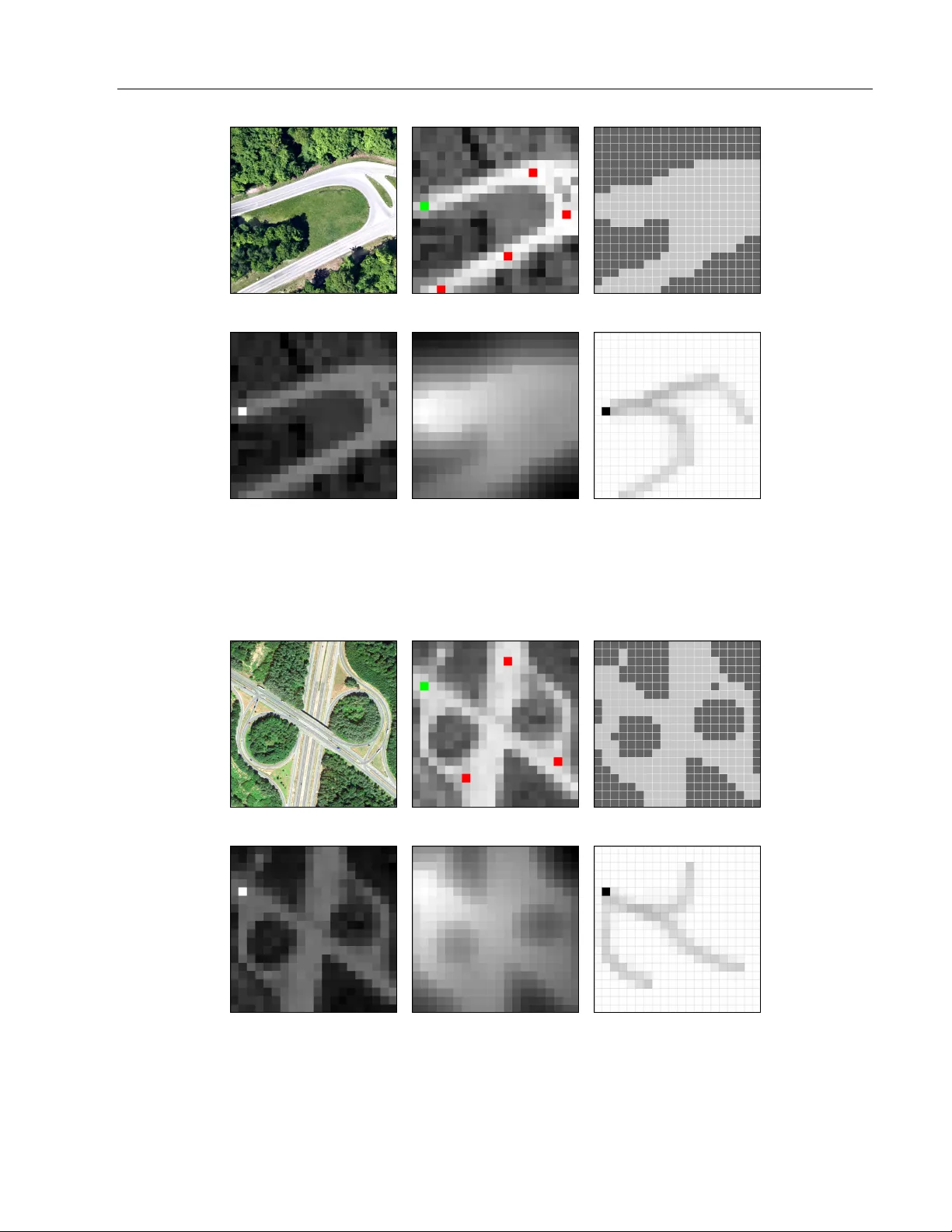
In v erse Reinforcemen t Learning with Sim ultaneous Estimation of Rew ards and Dynamics Mic hael Herman ? † T obias Gindele ? J¨ org W agner ? F elix Sc hmitt ? W olfram Burgard † ? Rob ert Bosc h GmbH D-70442 Stuttgart, German y † Univ ersity of F reiburg D-79110 F reiburg, Germany Abstract In verse Reinforcemen t Learning (IRL) de- scrib es the problem of learning an unkno wn rew ard function of a Marko v Decision Pro- cess (MDP) from observed behavior of an agen t. Since the agent’s b ehavior originates in its p olicy and MDP p olicies depend on b oth the sto chastic system dynamics as well as the rew ard function, the solution of the in verse problem is significantly influenced by b oth. Current IRL approac hes assume that if the transition mo del is unkno wn, additional samples from the system’s dynamics are ac- cessible, or the observed b ehavior provides enough samples of the system’s dynamics to solv e the inv erse problem accurately . These assumptions are often not satisfied. T o o ver- come this, we presen t a gradien t-based IRL approac h that simultaneously estimates the system’s dynamics. By solving the com bined optimization problem, our approach tak es in to account the bias of the demonstrations, whic h stems from the generating p olicy . The ev aluation on a synthetic MDP and a transfer learning task shows improv emen ts regarding the sample efficiency as well as the accuracy of the estimated reward functions and tran- sition mo dels. 1 In tro duction With more and more autonomous systems p erforming complex tasks in v arious applications, it is necessary to provide simple programming approaches for non- exp erts to adjust the systems’ abilities to new en viron- App earing in Pro ceedings of the 19 th In ternational Con- ference on Artificial Intelligence and Statistics (AIST A TS) 2016, Cadiz, Spain. JMLR: W&CP volume 51. Copyrigh t 2016 by the authors. men ts. A mathematical framework for mo deling deci- sion making under partly random outcomes are MDPs. By sp ecifying an environmen t, its dynamics and a re- w ard function, optimal p olicies can b e derived, e.g. b y reinforcemen t learning (RL) (Sutton and Barto, 1998). Ho wev er, when the environmen t or the problem gets complex, it is often difficult to sp ecify appropriate re- w ard functions that yield a desired b ehavior. Instead, it can be easier to provide demonstrations of the de- sired b ehavior. Therefore, Ng and Russell (2000) intro- duced Inv erse Reinforcement Learning (IRL), whic h describ es the problem of recov ering a reward function of an MDP from demonstrations. The basic idea of IRL is that the reward function is the most succinct representation of an exp ert’s ob jectiv e, whic h can b e easily transferred to new environmen ts. Man y approaches hav e been prop osed to solv e the IRL problem, such as (Abb eel and Ng, 2004; Ratliff et al., 2006; Neu and Szepesv´ ari, 2007; Ramachand ran and Amir, 2007; Rothkopf and Dimitrak akis, 2011). Since exp ert demonstrations are rarely optimal, IRL ap- proac hes hav e b een in tro duced that deal with sto chas- tic behavior, e.g. (Ziebart et al., 2008, 2010; Bloem and Bam b os, 2014). Most of these approaches hav e in common that they require the system’s dynamics to b e known. Since this assumption is often not satisfied, mo del-free IRL algorithms ha ve been proposed, suc h as (Boularias et al., 2011; T ossou and Dimitrak akis, 2013; Klein et al., 2012, 2013). As the mo del-based approaches need to rep eatedly solv e the RL problem as part of solving the IRL prob- lem, they require an accurate model of the system’s dynamics. Most of them assume that an MDP mo del including the dynamics is either giv en or can b e es- timated well enough from demonstrations. Ho wev er, as the observ ations are the result of an exp ert’s pol- icy , they only provide demonstrations of desired be- ha vior in desired states. As a consequence, it is often not p ossible to estimate an accurate transition mo del directly from exp ert demonstrations. Mo del-free ap- proac hes t ypically require that the observed demon- In verse Reinforcement Learning with Simultaneous Estimation of Rew ards and Dynamics strations con tain enough samples of the system’s dy- namics to accurately learn the rew ard function or re- quire access to the en vironment or a simulator to gen- erate additional data. How ev er, in many applications realistic sim ulators do not exist and it is not p ossible to query the en vironment. In this case, current model- free IRL approac hes either don’t consider rewards or transitions of unobserved states and actions, or tend to suffer from wrong generalizations due to heuristics. W e argue that sim ultaneously optimizing the lik eli- ho o d of the demonstrations with respect to the rew ard function and the dynamics of the MDP can impro v e the accuracy of the estimates and with it the result- ing p olicy . Even though man y transitions ha ve never b een observed, they can to some degree be inferred b y taking in to account that the data has b een gener- ated by an exp ert’s p olicy . Since the exp ert’s policy is the result of b oth his reward function and his b elief ab out the system’s dynamics, the frequency of state- action pairs in the data carries information ab out the exp ert’s ob jectiv e. This can b e exploited to improv e the sample efficiency and the accuracy of the estima- tion of the system’s dynamics and the reward function, as they b oth influence the p olicy . One side of this bi- lateral influence has b een used by Golub et al. (2013), who sho wed that more accurate dynamics can b e esti- mated when the rew ard function is known. Our contribution is integrating the learning of the transition mo del into the IRL framew ork, b y consider- ing that demonstrations hav e been generated based on a p olicy . This even allows dra wing conclusions ab out parts of the transition model that w ere never ob- serv ed. W e pro vide a general gradient-based solution for a simultaneous estimation of rewards and dynamics (SERD). F urthermore, w e deriv e a concrete algorithm, based on Maxim um Discoun ted Causal En tropy IRL (Blo em and Bambos, 2014). Part of it is an iterative computation of the p olicy gradient for which we sho w con vergence. W e ev aluate our approach on synthetic MDPs, compare it to model-based and mo del-free IRL approac hes, and test its generalization capabilities in a transfer task. More detailed deriv ations and proofs are pro vided in the supplementary material. 2 F undamen tals This section introduces the notation and fundamen tals to formulate the IRL problem with a simultaneous es- timation of rew ards and dynamics. 2.1 Mark ov Decision Processes An MDP is a tuple M = { S, A, P ( s 0 | s, a ) , γ , R, P ( s 0 ) } , where S is the state space with states s ∈ S , A is the action space with actions a ∈ A , P ( s 0 | s, a ) is the prob- abilit y of a transition to s 0 when action a is applied in state s , γ ∈ [0 , 1) is a discoun t factor, R : S × A → R is a reward function whic h assigns a real-v alued reward for picking action a in state s , and P ( s 0 ) is a start state probabilit y distribution. The goal of an MDP is to find an optimal p olicy π ∗ ( s, a ) = P ( a | s ), whic h specifies the probability of taking action a in state s , suc h that executing this p ol- icy maximizes the expected, discoun ted future reward: V π ( s ) = E " ∞ X t =0 γ t R ( s t , a t ) | s 0 = s, π # (1) If the p olicy is deterministic, the probability distri- bution can b e expressed with one single action v alue π ∗ d ( s ) = a . Additionally , a Q-function can b e defined, whic h sp ecifies the expected, discoun ted, cumulated rew ard for starting in state s , picking action a and then follo wing the p olicy π . Q π ( s, a ) = E " ∞ X t =0 γ t R ( s t , a t ) | s 0 = s, a 0 = a, π # (2) 2.2 In verse Reinforcemen t Learning IRL describ es the problem of learning the unknown rew ard function of an MDP from observed behavior of an agen t acting according to some stochastic policy . It is therefore characterized by the tuple M \ R and ob- serv ed demonstrations D = { τ 1 , τ 2 , . . . , τ N } with tra- jectories τ =  ( s τ 0 , a τ 0 ) , ( s τ 1 , a τ 1 ) , . . . ,  s τ T τ , a τ T τ  . The goal of IRL is to estimate the agen t’s reward func- tion R ( s, a ), whic h explains the observed b eha vior in the demonstrations. Often this reward is expressed as state- and action-dep endent features f : S × A → R d . An IRL mo del assuming sto chastic exp ert b ehavior is the Maximum Entrop y IRL (MaxEnt IRL) mo del of Ziebart et al. (2008), which has b een applied to differ- en t learning problems, such as (Ziebart et al., 2009; Henry et al., 2010; Kuderer et al., 2013). Since it do esn’t supp ort sto c hastic transition mo dels to the full exten t, Ziebart et al. (2010) proposed an approac h, called Maximum Causal Entrop y IRL (MCE IRL). Blo em and Bambos (2014) extended MCE IRL to the infinite time horizon case, which is called Maximum Discoun ted Causal En tropy IRL (MDCE IRL). They deriv e a simplified stationary soft v alue iteration solu- tion for MDCE IRL, whic h is formulated as V θ ( s ) = log X a ∈ A exp ( Q θ ( s, a )) ! (3) Mic hael Herman, T obias Gindele, J¨ org W agner, F elix Sc hmitt, W olfram Burgard where the soft state-action v alue Q θ ( s, a ) is defined as Q θ ( s, a ) = θ T f ( s, a ) + γ X s 0 ∈ S P ( s 0 | s, a ) V θ ( s 0 ) . (4) This soft v alue iteration is a con traction mapping, whic h has b een prov en in (Blo em and Bambos, 2014). The stochastic p olicy π θ ( s, a ) can b e extracted from the stationary fixed p oint solutions of V θ ( s ) and Q θ ( s, a ) and forms a Boltzmann distribution ov er the Q-v alues of all v alid actions in state s : π θ ( s, a ) = exp( Q θ ( s, a ) − V θ ( s )) = exp( Q θ ( s, a )) P a 0 ∈ A exp ( Q θ ( s, a 0 )) . (5) The linear combination of feature weigh ts θ ∈ R d and features f ( s, a ) ∈ R d in Eq. (4) can b e interpreted as a rew ard function R ( s, a ) = P d k =1 θ k f k ( s, a ). As the features are defined b y the states and actions, estimat- ing a reward function degrades to finding appropriate feature weigh ts. Due to the Mark ov assumption in MDPs it is possible to form ulate the probability of a sp ecific tra jectory τ based on the start distribution, the single actions and the transitions: P ( τ | M , θ ) = P ( s τ 0 ) T τ − 1 Y t =0  π θ ( s τ t , a τ t ) · P  s τ t +1 | s τ t , a τ t  . (6) Ziebart et al. hav e sho wn in (Ziebart, 2010; Ziebart et al., 2010) that appropriate feature weigh ts can be learned b y optimizing the lik elihoo d of the data un- der the maximum causal en trop y distribution p olicy π θ ( s, a ) from Eq. (5). Assuming indep endent tra jec- tories, the likelihoo d of the demonstrations in D can b e expressed as P ( D | M , θ ) = Y τ ∈ D P ( τ | M , θ ) . (7) Meaningful feature w eigh ts can then be found b y max- imizing the log-likelihoo d of the demonstrations with resp ect to the feature w eights θ : θ ∗ = argmax θ log P ( D | M , θ ) . (8) 3 Sim ultaneous Estimation of Rew ards and Dynamics (SERD) Man y IRL approac hes assume that the system dynam- ics are kno wn or can b e estimated w ell enough from demonstrations. T o the b est of our kno wledge, the ro- bustness of IRL against wrong transition mo dels has not b een studied so far, even though this problem has already b een p ointed out in (Ramachandran and Amir, 2007). Ho w ever, as the transition model influences the p olicy , the reward estimation of the IRL problem can b e falsified due to wrong transition mo del estimates. It ma y then b e adv an tageous to learn b oth at once, in order to capture the relationship b etw een the rew ard function and the dynamics mo del in the policy . Ad- ditionally , it is p ossible that the agent’s b elief about the system’s dynamics differs from the true one, which yields a wrong policy . This led us to the formulation of a new problem class, which can b e c haracterized as follo ws: Determine: • Agen t’s reward function R ( s, a ) • Agen t’s b elief ab out the dynamics P A ( s 0 | s, a ) • Real dynamics P ( s 0 | s, a ) Giv en • MDP M \ { R , P ( s 0 | s, a ) , P A ( s 0 | s, a ) } without the rew ard function or any dynamics • Demonstrations D of an agent acting in M based on a p olicy that depends on R ( s, a ) and P A ( s 0 | s, a ) T o solve this problem we prop ose an approach with a com bined estimation, called Simultaneous Estimation of Rewards and Dynamics (SERD). W e assume that there exist models for P ( s 0 | s, a ) and P A ( s 0 | s, a ), whic h can be parameterized. Therefore, we introduce a set of parameters, which should b e estimated from the given demonstrations D : θ R F eature weigh ts of the reward function R ( s, a ) θ T A P arameters of the agent’s transition mo del P θ T A θ T P arameters of the real transition mo del P θ T Since no prior information ab out rew ards or dynamics is known, our SERD approach for solving the problem is to maximize the likelihoo d of the demonstrations with resp ect to these parameters, whic h can b e com- bined in the parameter vector θ =  θ | R θ | T A θ | T  | . This is related to the approaches in (Ziebart, 2010; Ziebart et al., 2008), whic h estimates feature weigh ts θ R b y maximizing the log lik eliho o d of the demonstra- tions under the maxim um entrop y distribution p olicy π θ ( s, a ) of Eq. (5). Assuming independent tra jecto- ries, the lik eliho o d of the demonstrations in D can b e expressed as P ( D | M , θ ) = Y τ ∈ D P ( s τ 0 ) T τ − 1 Y t =0  π θ ( s τ t , a τ t ) · P θ T  s τ t +1 | s τ t , a τ t  . (9) In verse Reinforcement Learning with Simultaneous Estimation of Rew ards and Dynamics W e wan t to p oint out that the p olicy π θ ( s, a ) dep ends on b oth feature weigh ts θ R as well as the agent’s dy- namics parameters θ T A , whereas the transition mo del P θ T ( s 0 | s, a ) only dep ends on θ T . The log lik eliho o d of the demonstrations L θ ( D ) can then be derived from Eq. (9): L θ ( D ) = log P ( D | M , θ ) (10) = X τ ∈ D " log P ( s τ 0 ) + T τ − 1 X t =0  log π θ ( s τ t , a τ t ) + log P θ T  s τ t +1 | s τ t , a τ t  # . (11) Solving the SERD problem then corresp onds to opti- mizing the log likelihoo d of the demonstrations with resp ect to θ , which is formulated as: θ ∗ = argmax θ L θ ( D ) . (12) W e prop ose a gradien t-based metho d to optimize the log lik eliho o d of Eq. (11), whic h shares similarities with the approach in (Neu and Szep esv´ ari, 2007). Therefore, w e deriv e the gradien t ∇ θ L θ ( D ) to solv e the SERD problem of Eq. (12). This gradient can b e formalized as: ∇ θ L θ ( D ) = X τ ∈ D T τ − 1 X t =0  ∇ θ log π θ ( s τ t , a τ t ) + ∇ θ log P θ T  s τ t +1 | s τ t , a τ t  . (13) As the start state distribution do es not dep end on any of the parameters θ the term P τ ∈ D log P ( s τ 0 ) v anishes. The gradient ∇ θ L θ ( D ) can therefore b e factorized to cum ulated gradients of the state-action pair proba- bilit y ∇ θ log π θ ( s τ t , a τ t ) and the transition probability ∇ θ log P θ T  s τ t +1 | s τ t , a τ t  . Since the gradient of the true transition probability is mo del dep endent, the follo w- ing deriv ations will fo cus on the gradien t of the p olicy ∇ θ log π θ ( s τ t , a τ t ). Usually , this p olicy is problem sp e- cific, which requires to sp ecify an IRL type. W e will deriv e the gradient for MDCE IRL, but an extension to further IRL solutions and p olicies is p ossible. 4 Maxim um Discounted Causal En trop y SERD (MDCE-SERD) In the follo wing, w e will exemplarily derive the gra- dien t of p olicies ∇ θ log π θ ( s τ t , a τ t ) that are based on MDCE IRL by Blo em and Bambos (2014), whic h has b een in troduced in Section 2.2. Under this assumption the partial deriv ativ e of the p olicy can b e decomp osed b y replacing π θ ( s τ t , a τ t ) through its represen tation in MDCE IRL: ∂ ∂ θ i log π θ ( s, a ) = ∂ ∂ θ i Q θ ( s, a ) − E π θ ( s,a 0 )  ∂ ∂ θ i Q θ ( s, a 0 )  . (14) It follows that the gradien t of the policy de- p ends on the gradien t of the state-action v alue function ∂ ∂ θ i Q θ ( s, a ) and the expected gradient E π θ ( s,a 0 ) h ∂ ∂ θ i Q θ ( s, a 0 ) i . As the exp ectation is taken with respect to the stochastic p olicy π θ ( s, a 0 ), which dep ends on the Q-function, a basic requiremen t for its computation is a conv erged Q- and v alue-function. In the follo wing, we will provide the partial deriv ative of the iterativ e soft Q-function with resp ect to θ i , whic h w e call soft Q-gradien t. The partial deriv atives with resp ect to the individual parameter types, such as fea- ture weigh ts or transition parameters, can b e found in the supplemen t. ∂ ∂ θ i Q θ ( s, a ) = ∂ ∂ θ i θ | R f ( s, a ) (15) + γ X s 0 ∈ S  ∂ ∂ θ i P θ T A ( s 0 | s, a )  V θ ( s 0 )  (16) + γ X s 0 ∈ S  P θ T A ( s 0 | s, a ) · E π θ ( s 0 ,a 0 )  ∂ ∂ θ i Q θ ( s 0 , a 0 )  (17) The soft Q-gradien t computation is a linear equation system and can thus b e computed directly . Nev erthe- less, if the num ber of parameters is large, it can b e b eneficial to choose an iterative approach. F or this purp ose, Eq. (17) can b e interpreted as a recursiv e function, whic h we call soft Q-gradient iteration. The first tw o terms (15) and (16) are constants due to the requiremen t of a static and conv erged soft Q-function. The third term (17) propagates exp ected gradients through the space of states S , actions A , and parame- ter dimensions θ . The partial deriv ativ e ∂ ∂ θ i Q θ ( s, a ) is a fixed p oint iteration and can therefore b e computed b y starting with arbitrary gradien ts and recursiv ely applying Eq. (17). W e will prov e this in section 4.1. Solving the linear system of Eq. (17) with | S | states, | A | actions, and N θ parameters directly via LU de- comp ositions requires O  N θ · ( | S | · | A | ) 3  computa- tions. Instead, a single iteration of Eq. (17) requires O  N θ · ( | S | · | A | ) 2  computations, which can b e b en- eficial if the n umber of states and actions is large. Ad- ditionally , the result of the soft Q-iteration can b e used to initialize a subsequent soft Q-iteration with slightly c hanged parameters to further decrease the num b er of necessary iterations. Mic hael Herman, T obias Gindele, J¨ org W agner, F elix Sc hmitt, W olfram Burgard Algorithm 1 summarizes the MDCE-SERD algorithm. The function DynamicsEstimator provides a naiv e dy- namics estimate from the transitions of the demon- strations. SoftQIter ation p erforms the soft Q-iteration from Eq. (3) and (4) un til conv ergence. DerivePolicy p erforms a policy up date based on the policy defini- tion in Eq. (5) and the function SoftQGr adientIter a- tion solves the soft Q-gradient iteration from Eq. (17) un til conv ergence. Then, the function ComputeGr adi- ent calculates the gradient based on Eq. (13). Algorithm 1 MDCE-SERD algorithm Require: MDP M \ { R, P T , P T A } , Demonstrations D , initial ˜ θ , step size α : N + → R + , t ← 0 θ 0 ← DynamicsEstimator( M , D , ˜ θ ) while not sufficiently conv erged do Q θ ← SoftQIteration( M , θ t ) π θ ← Deriv ePolicy( M , Q θ ) d Q θ ← SoftQGradien tIteration( M , Q θ , π θ , θ t ) ∇ θ L θ ( D ) ← ComputeGradien t( M , D , d Q θ ) θ t +1 ← θ t + α ( t ) ∇ θ L θ ( D ) t ← t + 1 end while 4.1 Pro ofs T o pro ve the correctness and conv ergence of the pro- p osed algorithm, it must be shown that the soft Q- iteration is a contraction mapping, that the soft Q- function is differentiable, and that the soft Q-gradient iteration is a contraction mapping. Blo em and Bam- b os (2014) hav e sho wn that the soft v alue iteration op- erator is a contraction mapping. The proof for the soft Q-iteration is straigh tforward and is presented in the supplemen tary material together with more detailed deriv ations for all pro ofs. Theorem 4.1. The soft Q-iter ation op er ator T sof t θ ( Q ) is a c ontr action mapping with only one fixe d p oint. Ther efor e, it is Lipschitz c ontinuous || T sof t θ ( Q m ) − T sof t θ ( Q n ) || ∞ ≤ L || Q m − Q n || ∞ for al l Q m , Q n ∈ R | S |×| A | with a Lipschitz c onstant L = γ ∈ [0 , 1) . Theorem 4.2. The c onver ge d soft Q-function is dif- fer entiable with r esp e ct to θ . The soft Q-gradient op erator U sof t θ ( Φ ) ∈ R | S |×| A |×| Ψ | is defined as: U sof t θ ( Φ )( s, a, i ) = ∂ ∂ θ i θ | R f ( s, a ) + γ X s 0 ∈ S  ∂ ∂ θ i P θ T A ( s 0 | s, a )  V θ ( s 0 )  + γ X s 0 ∈ S n P θ T A ( s 0 | s, a ) · E π θ ( s 0 ,a 0 ) [Φ( s 0 , a 0 , i )] o , for all s ∈ S, a ∈ A and parameter dimensions i ∈ Ψ with Ψ = { 1 , . . . , dim( θ ) } and the gradient Φ( s, a, i ) = ∂ ∂ θ i Q θ ( s, a ) . Some auxiliary lemmata and definitions are necessary to prov e that the Q-gradien t iteration is a contrac- tion mapping. In order to argue ab out the monotonic- it y of m ultidimensional functions, a partial order on R A × B × C is in tro duced. The monotonicit y of the op- erator U sof t θ ( Φ ) with resp ect to the introduced partial order is pro ven. Definition 4.3. F or x , y ∈ R A × B × C with A, B , C ∈ N + , the p artial or der  is define d as x  y ⇔ ∀ a ∈ A, b ∈ B , c ∈ C : x a,b,c ≤ y a,b,c . Lemma 4.4. The soft Q-gr adient iter ation op er ator U sof t θ ( Φ )( s, a, i ) is monotone, satisfying ∀ Φ m , Φ n ∈ R | S |×| A |×| Ψ | : Φ m  Φ n → U sof t θ ( Φ m )  U sof t θ ( Φ n ) . Pr o of. The partial deriv ative of the U sof t θ ( Φ )( s, a, i ) with resp ect to a single v alue Φ( s k , a k , k ) is ∂ ∂ Φ( s k , a k , k ) U sof t θ ( Φ )( s, a, i ) = ∂ ∂ Φ( s k , a k , k ) γ X s 0 ∈ S n P θ T A ( s 0 | s, a ) · E π θ ( s 0 ,a 0 ) [Φ( s 0 , a 0 , i )] o = γ P θ T A ( s k | s, a ) π θ ( s k , a k ) . F rom the definition of the MDP it follows that γ ∈ [0 , 1) and the probabilit y distributions P θ T A ( s i | s, a ) ∈ [0 , 1] as w ell as π θ ( s k , a k ) ∈ [0 , 1]. Since all terms of the partial deriv ative ∂ ∂ Φ( s k ,a k ,k ) U sof t θ ( Φ )( s, a, i ) are p ositive or zero, it fol- lo ws that ∂ ∂ Φ( s k ,a k ,k ) U sof t θ ( Φ )( s, a, i ) ≥ 0. Theorem 4.5. The soft Q-gr adient iter ation op er a- tor U sof t θ ( Φ )( s, a, i ) is a c ontr action mapping with only one fixe d p oint. Ther efor e, it is Lipschitz c ontinuous || U sof t θ ( Φ m ) − U sof t θ ( Φ n ) || ∞ ≤ L || Φ m − Φ n || ∞ for al l Φ m , Φ n ∈ R | S |×| A |×| Ψ | with a Lipschitz c onstant L ∈ [0 , 1) . Pr o of. Consider Φ m , Φ n ∈ R | S |×| A |×| Ψ | . There exists a distance d under the supremum norm, for which ∃ d ∈ R + 0 : || Φ m − Φ n || ∞ = d holds and therefore − d 1  Φ m − Φ n  − d 1 with 1 = (1) k,l,m , where 1 ≤ k ≤ | S | , 1 ≤ l ≤ | A | , 1 ≤ m ≤ | Ψ | . By adding d to every elemen t of Φ n it is guaran teed that Φ m  Φ n + d 1 . Therefore, the monotonicity condition of Lemma 4.4 is satisfied: U sof t θ ( Φ m )  U sof t θ ( Φ n + d 1 ). Then, it In verse Reinforcement Learning with Simultaneous Estimation of Rew ards and Dynamics follo ws ∀ s ∈ S, a ∈ A, i ∈ Ψ : U sof t θ ( Φ m )( s, a, i ) ≤ U sof t θ ( Φ n + d 1 )( s, a, i ) = ∂ ∂ θ i θ | R f ( s, a ) + γ X s 0 ∈ S  ∂ ∂ θ i P θ T A ( s 0 | s, a )  V θ ( s 0 )  + γ X s 0 ∈ S n P θ T A ( s 0 | s, a ) E π θ ( s 0 ,a 0 ) [Φ( s 0 , a 0 , i ) + d ] o = ∂ ∂ θ i θ | R f ( s, a ) + γ X s 0 ∈ S  ∂ ∂ θ i P θ T A ( s 0 | s, a )  V θ ( s 0 )  + γ X s 0 ∈ S n P θ T A ( s 0 | s, a ) E π θ ( s 0 ,a 0 ) [Φ( s 0 , a 0 , i )] o + γ d = U sof t θ ( Φ n )( s, a, i ) + γ d In vector notation this results in U sof t θ ( Φ m )  U sof t θ ( Φ n ) + γ d 1 . F rom the symmetric definition of d it equally follo ws that Φ n  Φ m + d and conse- quen tly U sof t θ ( Φ n )  U sof t θ ( Φ m ) + γ d 1 . By com bining these inequations, the Lipschitz contin uit y of the soft Q-gradien t iteration can b e shown: γ d 1  U sof t θ ( Φ m ) − U sof t θ ( Φ n )  γ d 1 || U sof t θ ( Φ m ) − U sof t θ ( Φ n ) || ∞ ≤ γ d || U sof t θ ( Φ m ) − U sof t θ ( Φ n ) || ∞ ≤ γ || Φ m − Φ n || ∞ This prov es that the soft Q-gradient iteration oper- ator U sof t θ ( Φ )( s, a, i ) is Lipschitz con tinuous with a Lipsc hitz constant L = γ and γ ∈ [0 , 1), resulting in a con traction mapping. As this holds for the whole input space R | S |×| A |×| Ψ | , t wo p oints would alw ays contract, so there cannot exist t wo fixed p oints. 5 Related W ork In prior w ork v arious mo del-free and mo del-based IRL approac hes hav e b een prop osed. Ziebart et al. (2008) prop osed MaxEnt IRL in an early work, where a max- im um en tropy probabilit y distribution of tra jectories is trained to matc h feature expectations. One dra w- bac k of MaxEn t IRL is that it do es not accoun t for sto c hastic transition mo dels to the full extent. There- fore, Ziebart et al. (2010) extended the previous ap- proac h to MCE IRL, whic h allows for sto chastic tran- sition mo dels. Both algorithms require the transi- tion mo del of the MDP to b e known and are com- putationally exp ensive, since they need to repeatedly solv e the RL problem. Therefore, mo del-free IRL ap- proac hes ha ve b een proposed, whic h ov ercome this requiremen t. Boularias et al. (2011) prop ose an ap- proac h called Relative Entrop y IRL (REIRL), which minimizes the Kullback-Leibler divergence b etw een a learned tra jectory distribution and one that is based on a baseline p olicy under the constraint to match feature exp ectations. F or this purp ose, the baseline p olicy is approximated via imp ortance sampling from arbitrary p olicies. Since the problem formulation of REIRL originates from MaxEnt IRL, it do es not in- herit the adv antages of MCE IRL and thus can b e inappropriate for sto c hastic domains. How ev er, sim- ilarly to MaxEnt IRL and MCE IRL, it allows for sto c hastic agent b ehavior. A disadv antage of REIRL is its requirement for non-exp ert demonstrations from an arbitrary policy . Klein et al. (2012) reformulate the IRL problem as a structured classification of ac- tions given state- and action-dependent feature coun ts that are estimated from the dem onstrations (SCIRL). Missing feature coun ts are obtained by querying addi- tional samples of non-optimal actions or by in tro duc- ing heuristics. How ever, SCIRL can only b e applied if the agent has b een following a deterministic p olicy . Instead, the MDCE-SERD approac h in this pap er can train mo dels from sub optimal demonstrations. In ad- dition to reward learning in IRL, it optimizes the tran- sition mo del. A disadv antage of MDCE-SERD is that it needs to repeatedly solv e the forw ard problem and the soft Q-iteration. How ever, learning b etter rew ard functions and transition mo dels is esp ecially b eneficial if both need to b e transferred to new en vironments, where it is not p ossible to query new demonstrations. In suc h cases, more accurate mo dels will result in b et- ter p olicies. 6 Ev aluation W e ev aluated the MDCE-SERD approac h in a grid w orld na vigation task based on satellite images with differing sto c hastic motion dynamics in forest and op en terrain. F urthermore, w e tested its generaliza- tion capabilities in a transfer learning task. Therefore, w e transferred the estimated transition mo del and the rew ard function to another satellite image and com- parred the resulting p olicy to the true one. In the learning part of the ev aluation, the aim of an agen t should be learned solely from demonstrations of a na v- igation task in a sto chastic environmen t. Figure 1 il- lustrates the settings of the tasks. In each state the agen t can choose from five different actions, which are mo ving in one of four directions (north, east, south, or west) or staying in the state. The set of successor states is restricted to the curren t state and the four neigh b oring states. On the op en terrain (Fig. 1 (c): depicted in ligh t gra y) the agent successfully executes a motion action with probabilit y 0 . 8 and falls with 0 . 1 to either right or left of the desired direction. The agent’s dynamics in the forest (Fig. 1 (c): depicted in dark gray) are more sto c hastic. Successful transitions o ccur with probabil- Mic hael Herman, T obias Gindele, J¨ org W agner, F elix Sc hmitt, W olfram Burgard (a) (b) (c) (d) (e) (f ) Figure 1: The first row represents the test task and the second row the transfer task. (a) Environmen t, Map data: Google. (b) Discretized state space. The goal state is indicated in green and start states in red. (c) F orest states are indicated in a dark-gray color and op en terrain in light gra y . F urthermore, plot (d) shows the reward, (e) the resulting v alue function, and (f ) the exp ected state frequency . it y 0 . 3, otherwise the agent randomly falls into one of the remaining successor states. As a consequence the agen t has to trade off short cuts through the forest against longer paths on the open terrain that are more lik ely to be successful. Staying in a state is alw ays suc- cessful. The rew ard function is a linear combination of tw o state-dependent features. One of them is the gra y scale v alue of the image, which has b een normal- ized to [0 , 1], the other is a goal iden tity , b eing 1 in the goal state and 0 otherwise. The feature w eights of the true mo del were set to θ R = (6 , 6) | and the discoun t to 0 . 99. Fig. 1 (d) illustrates the resulting rew ard function, which fav ors roads and esp ecially the goal state. W e computed the stochastic policy of this MDP ac- cording to Eq. (5). Then, w e sampled tra jectories from the resulting p olicy , whic h w ere used as train- ing samples for the ev aluation of the learning task. Since the MDCE p olicy is sto chastic, sub optimal ex- p ert b ehavior is considered. F or learning, we assumed that the exp ert has complete knowledge ab out the true dynamics, so that θ T A and θ T are equal. This mak es it possible to use b oth terms of Eq. (13) to optimize the transition mo del parameters. W e esti- mate indep endent transition mo dels for each action (north, east, south, and west) b oth in the forest and the op en terrain, as well as a shared mo del for stay- ing. Therefore, 9 mo dels are trained with 5 possible outcomes, resulting in 45 transition mo del parameters that are energies of Boltzmann distributions. W e used an m-estimator with a uniform prior to estimate inde- p enden t dynamics for eac h action from the observ ed transitions. Then, mo dels hav e b een trained from the demonstrations based on random feature weigh t ini- tializations ( ∀ i : θ i ∈ [ − 10 , 10]) with MDCE IRL, REIRL, and MDCE-SERD for v arious sizes of demon- stration sets. A requiremen t of REIRL are samples from a arbitrary known p olicy , suc h that the IRL prob- lem can b e solv ed with imp ortance sampling. Since only exp ert demonstrations are av ailable, these sam- ples are generated based on the dynamics estimate and an m-estimated p olicy from the exp erts demon- strations. This results in meaningful tra jectories and more accurate REIRL estimates. Figure 2 summarizes the results of the ev aluation for v arying num b ers of exp ert demonstrations. The first figure illustrates the a verage log likelihoo d of demonstrations from the true mo del on the learned ones, where MDCE-SERD outp erforms the other ap- proac hes and needs muc h fewer demonstrations to ob- tain go o d estimates. The increase in p erformance of MDCE-SERD ov er MDCE IRL is explained by the fact that it can adjust wrongly estimated tran- sition mo dels. It is interesting to note that REIRL p erformed w orse than MDCE IRL. This is probably caused b y the fact that REIRL is based on MaxEn t IRL (Ziebart et al., 2008), whic h do esn’t consider the transitition sto c hasticity to the full extent. This can falsify the learning, esp ecially , if the sto chasticit y in- fluences the agent’s b ehavior. Figure 2 (b) shows the a verage Kullback-Leibler divergence b etw een the esti- mated transition model and the real one. The tran- sition mo dels of REIRL and MDCE IRL hav e b een deriv ed by an m-estimator from the given demonstra- tions and therefore p erform similarly . The transition mo del of MDCE-SERD has b een further optimized si- m ultaneously with the rew ards, resulting in more ac- curate transition mo dels. Figure 2 (c) illustrates the In verse Reinforcement Learning with Simultaneous Estimation of Rew ards and Dynamics 20 40 60 80 100 120 − 50 − 40 − 30 − 20 | D | logP ( D | M ) MDCE IRL REIRL MDCE-SERD (a) Log likelihoo d of the demonstrations 20 40 60 80 100 120 10 − 5 10 − 4 10 − 3 | D | E [ D K L ( P T || P T A )] MDCE IRL REIRL MDCE-SERD (b) KL divergence of the transition mo del 20 40 60 80 100 120 10 − 2 10 0 | D | E [ D K L ( π θ || π )] MDCE IRL REIRL MDCE-SERD (c) KL divergence of the p olicy 20 40 60 80 100 120 − 40 − 35 − 30 − 25 | D | logP ( D | M ) MDCE IRL REIRL MDCE-SERD (d) Log likelihoo d of the demonstrations (transfer) Figure 2: (a) Av erage log likelihoo d of demonstrations dra wn from the true mo del under the estimated mo del. (b) Av erage Kullback-Leibler divergence b etw een the estimated dynamics and the true ones. (c) Av erage Kullback- Leibler divergence b etw een the trained sto c hastic p olicy and the true one. (d) Av erage log lik eliho o d of demon- strations dra wn from the true mo del under the estimated mo del in the transfer task environmen t. Kullbac k-Leibler div ergence of the estimated p olicy , where MDCE-SERD outp erforms b oth MDCE IRL and REIRL. Then, the estimated mo dels from the learning task ha ve b een tranferred to the transfer task environ- men t, where a p olicy has b een computed based on the learned reward function and the estimated tran- sition mo del. Figure 2 (d) shows the av erage log lik e- liho o d of demonstrations from the true mo del under the estimated one. MDCE SERD shows an improv ed p erformance against the other approaches, probably b ecause it could more accurately estimate the mo del and therefore generates b etter policies. Therefore, it can b e concluded that if the transition mo del and the rew ard function are transfered to a new environmen t, where the agent suddenly acts in states and actions that hav e nev er or rarely been observ ed, more accu- rate mo dels can help to generate meaningful p olicies. 7 Conclusion In this paper w e inv estigated the new problem class of IRL, where b oth the rew ard function and the sys- tem’s dynamics are unkno wn and need to b e estimated from demonstrations. W e presen ted a gradient-based solution, which simultaneously estimates parameters of the transition mo del and the reward function by taking into accoun t the bias of the demonstrations. T o the b est of our knowledge, this has not b een con- sidered previously and is not p ossible with current ap- proac hes. The ev aluation sho ws that the com bined ap- proac h estimates mo dels more accurately than MDCE IRL or REIRL, esp ecially in the case of limited data. This is esp ecially b eneficial if both the rew ard func- tion and the transition mo del are transferred to new en vironments, since the optimal p olicy could result in high frequencies of states and actions that were never or rarely observed. In addition, the estimated transi- tion mo del can b e of interest on its own. F uture work could extend SERD to partially observ able domains or contin uous state and action spaces. F urthermore, prior information about rew ards or dynamics can be easily introduced, by estimating only a subset of pa- rameters. This allows solving subproblems such as es- timating the dynamics for giv en rew ards. An aspect of our approach that can b e further exploited is the dis- crimination b etw een the true system’s dynamics and the exp ert’s estimate of it. Examining the relation- ship b et ween the t wo could be used to further impro ve the estimates and even yield p olicies that exceed the exp ert’s p erformance. Mic hael Herman, T obias Gindele, J¨ org W agner, F elix Sc hmitt, W olfram Burgard References Pieter Abb eel and Andrew Y. Ng. Appren ticeship learning via inv erse reinforcement learning. In Pr o- c e e dings of the Twenty-first International Confer- enc e on Machine L e arning , ICML ’04, New Y ork, NY, USA, 2004. A CM. Mic hael Blo em and Nicholas Bambos. Infinite time horizon maximum causal entrop y in verse reinforce- men t learning. In 53r d IEEE Confer enc e on De- cision and Contr ol, CDC 2014, L os Angeles, CA, USA, De c emb er 15-17, 2014 , pages 4911–4916, 2014. Ab deslam Boularias, Jens Kob er, and Jan P eters. Rel- ativ e entrop y in verse reinforcement learning. In Pr o c e e dings of F ourte enth International Confer enc e on A rtificial Intel ligenc e and Statistics (AIST A TS 2011) , 2011. Matthew Golub, Steven Chase, and Byron Y u. Learn- ing an in ternal dynamics mo del from control demon- stration. In ICML (1) , v olume 28 of JMLR Pr o c e e d- ings , pages 606–614. JMLR.org, 2013. P eter Henry , Christian V ollmer, Brian F erris, and Di- eter F ox. Learning to na vigate through crowded en- vironmen ts. In R ob otics and A utomation (ICRA), 2010 IEEE International Confer enc e on , pages 981– 986, 2010. Edouard Klein, Matthieu Geist, Bilal Piot, and Olivier Pietquin. Inv erse Reinforcement Learning through Structured Classification. In A dvanc es in Neur al In- formation Pr o c essing Systems (NIPS 2012) , Lake T aho e (NV, USA), December 2012. Edouard Klein, Bilal Piot, Matthieu Geist, and Olivier Pietquin. A cascaded sup ervised learning approach to in verse reinforcement learning. In Pr o c e e dings of the Eur op e an Confer enc e on Machine L e arning and Principles and Pr actic e of Know le dge Disc overy in Datab ases (ECML/PKDD 2013) , Prague (Czech Republic), Septem b er 2013. Markus Kuderer, Henrik Kretzschmar, and W olfram Burgard. T eac hing mobile rob ots to co op eratively na vigate in populated environmen ts. In Pr o c. of the IEEE/RSJ International Confer enc e on Intel ligent R ob ots and Systems (IROS) , T okyo, Japan, 2013. Gergely Neu and Csaba Szep esv´ ari. Appren ticeship learning using inv erse reinforcement learning and gradien t metho ds. In UAI 2007, Pr o c e e dings of the Twenty-Thir d Confer enc e on Unc ertainty in Artifi- cial Intel ligenc e, V anc ouver, BC, Canada, July 19- 22, 2007 , pages 295–302, 2007. Andrew Y. Ng and Stuart J. Russell. Algorithms for in verse reinforcemen t learning. In Pr o c e e dings of the Sevente enth International Confer enc e on Machine L e arning , ICML ’00, pages 663–670, San F rancisco, CA, USA, 2000. Morgan Kaufmann Publishers Inc. Deepak Ramachandran and Eyal Amir. Bay esian In- v erse Reinforcement Learning. Pr o c e e dings of the 20th International Joint Confer enc e on Artific al In- tel ligenc e , 51:2586–2591, 2007. Nathan D. Ratliff, J. Andrew Bagnell, and Martin A. Zink evich. Maximum margin planning. In Pr o- c e e dings of the 23r d International Confer enc e on Machine L e arning , ICML ’06, pages 729–736, New Y ork, NY, USA, 2006. ACM. Constan tin A. Rothk opf and Christos Dimitrak akis. Preference elicitation and in verse reinforcement learning. In ECML/PKDD (3) , volume 6913 of L e ctur e Notes in Computer Scienc e , pages 34–48. Springer, 2011. Ric hard S. Sutton and Andrew G. Barto. R einfor c e- ment le arning: An intr o duction , volume 116. Cam- bridge Univ Press, 1998. Aristide C. Y. T ossou and Christos Dimitrak akis. Probabilistic inv erse reinforcemen t learning in un- kno wn environmen ts. In Pr o c e e dings of the Twenty- Ninth Confer enc e on Unc ertainty in Artificial Intel- ligenc e, Bel levue, W A, USA, August 11-15, 2013 , 2013. Brian D. Ziebart. Mo deling purp oseful adaptive b e- havior with the principle of maximum c ausal en- tr opy . PhD thesis, Mac hine Learning Department, Carnegie Mellon Univ ersity , Pittsburgh, P A, USA, Dec 2010. AAI3438449. Brian D. Ziebart, Andrew Maas, J. Andrew (Drew) Bagnell, and Anind Dey . Maxim um entrop y inv erse reinforcemen t learning. In Pr o c e e ding of AAAI 2008 , July 2008. Brian D. Ziebart, Nathan Ratliff, Garratt Gallagher, Christoph Mertz, Kevin Peterson, J. Andrew Bag- nell, Martial Heb ert, Anind K. Dey , and Siddhartha Sriniv asa. Planning-based prediction for p edestri- ans. In Pr o c. of the International Confer enc e on Intel ligent R ob otsi and Systems , 2009. Brian D. Ziebart, J. Andrew Bagnell, and Anind K. Dey . Modeling interaction via the principle of max- im um causal en tropy . In Pr o c. of the International Confer enc e on Machine L e arning , pages 1255–1262, 2010. In v erse Reinforcemen t Learning with Sim ultaneous Estimation of Rew ards and Dynamics - Supplemen tary Material Mic hael Herman ? † T obias Gindele ? J¨ org W agner ? F elix Schmitt ? W olfram Burgard † ? Rob ert Bosc h GmbH D-70442 Stuttgart, German y † Univ ersity of F reiburg D-79110 F reiburg, Germany Abstract This do cument contains supplemen tary ma- terial to the pap er Inverse R einfor c ement L e arning with Simultane ous Estimation of R ewar ds and Dynamics with more detailed deriv ations, additional pro ofs to lemmata and theorems as well as larger illustrations and plots of the ev aluation task. 1 P artial Deriv ativ e of the P olicy ∂ ∂ θ i log π θ ( s, a ) = ∂ ∂ θ i ( Q θ ( s, a ) − V θ ( s )) = ∂ ∂ θ i Q θ ( s, a ) − log X a 0 ∈ A exp ( Q θ ( s, a 0 )) ! = ∂ ∂ θ i Q θ ( s, a ) − ∂ ∂ θ i log X a 0 ∈ A exp ( Q θ ( s, a 0 )) = ∂ ∂ θ i Q θ ( s, a ) − P a 0 ∈ A h exp ( Q θ ( s, a 0 )) ∂ ∂ θ i Q θ ( s, a 0 ) i P a 0 ∈ A exp ( Q θ ( s, a 0 )) = ∂ ∂ θ i Q θ ( s, a ) − E π θ ( s,a 0 )  ∂ ∂ θ i Q θ ( s, a 0 )  . App earing in Pro ceedings of the 19 th In ternational Con- ference on Artificial Intelligence and Statistics (AIST A TS) 2016, Cadiz, Spain. JMLR: W&CP volume 51. Copyrigh t 2016 by the authors. 2 P artial Deriv ativ e of the Soft Q-F unction with Resp ect to the Individual P arameter Types The partial deriv ative can b e further simplified if it is tak en with resp ect to the three individual param- eter types: the feature w eights, the agen t’s dynamics parameters, and the parameters of the true en viron- men t’s dynamics: ∀ θ i ∈ θ R : ∂ ∂ θ i Q θ ( s, a ) = f i ( s, a ) + γ X s 0 ∈ S  P θ T A ( s 0 | s, a ) E π θ ( s 0 ,a 0 )  ∂ ∂ θ i Q θ ( s 0 , a 0 )  ∀ θ i ∈ θ T A : ∂ ∂ θ i Q θ ( s, a ) = γ X s 0 ∈ S  ∂ ∂ θ i P θ T A ( s 0 | s, a )  V θ ( s 0 )  + γ X s 0 ∈ S  P θ T A ( s 0 | s, a ) E π θ ( s 0 ,a 0 )  ∂ ∂ θ i Q θ ( s 0 , a 0 )  ∀ θ i ∈ θ T : ∂ ∂ θ i Q θ ( s, a ) = 0 3 Pro of: Soft Q-iteration is a Con traction Mapping It has to b e shown that the soft Q-iteration is a fixed p oin t iteration with only one fixed p oin t, since this is a requirement of our algorithm. Bloem et al. hav e sho wn in Blo em and Bambos (2014) that the soft v alue iteration op erator is a contraction mapping. It has to b e prov en that the same holds for the soft Q-iteration op erator T sof t θ ( Q ). Therefore, w e adjust their pro of to b e v alid for the Q-iteration. In verse Reinforcement Learning with Simultaneous Estimation of Rew ards and Dynamics The soft Q-iteration op erator is defined as T sof t θ ( Q )( s, a ) = θ | R f ( s, a ) + γ X s 0 ∈ S  P θ T A ( s 0 | s, a ) softmax a 0 ∈ A ( Q ( s 0 , a 0 ))  with the function softmax x i ∈ x ( x i ) = log N X i =1 exp ( x i ) ! . W e will b egin with deriving pro ofs for necessary auxil- iary definitions and lemmata. In order to argue ab out the monotonicit y of m ultidimensional functions, a par- tial order on R A × B is introduced. Then, a prop- ert y of the softmax function is derived and afterw ards the monotonicity of the op erator T sof t θ ( Q )( s, a ) : R | S |×| A | → R | S |×| A | with resp ect to the in tro duced partial order is pro ven. Definition 3.1. F or x , y ∈ R A × B with A, B ∈ N + , the p artial or der  is define d as x  y ⇔ ∀ a ∈ A, b ∈ B : x a,b ≤ y a,b . Lemma 3.2. The softmax function has the pr op- erty that for any x ∈ R N and d ∈ R it holds that softmax x i ∈ x ( x i + d ) = softmax x i ∈ x ( x i ) + d . Pr o of. The prop erty can be easily shown by extracting the v ariable d from the softmax formulation: softmax x i ∈ x ( x i + d ) = log N X i =1 exp ( x i + d ) ! = log exp ( d ) N X i =1 exp ( x i ) ! = log N X i =1 exp ( x i ) ! + log (exp ( d )) = log N X i =1 exp ( x i ) ! + d = softmax x i ∈ x ( x i ) + d Lemma 3.3. The soft Q-iter ation op er ator T sof t θ ( Q )( s, a ) is monotone, satisfying ∀ Q m , Q n ∈ R | S |×| A | : Q m  Q n → T sof t θ ( Q m )  T sof t θ ( Q n ) . Pr o of. The partial deriv ative of the T sof t θ ( Q )( s, a ) with resp ect to a single v alue Q ( s i , a i ) is ∂ ∂ Q ( s i , a i ) T sof t θ ( Q )( s, a ) = γ P θ T A ( s i | s, a ) exp ( Q ( s i , a i )) P a j ∈ A exp ( Q ( s i , a j )) . F rom the definition of the MDP it follows that γ ∈ [0 , 1) and the probability distribution P θ T A ( s i | s, a ) ∈ [0 , 1]. As ∀ x i ∈ R : exp( x i ) ∈ (0 , + ∞ ), all terms of the partial deriv ative ∂ ∂ Q ( s i ,a i ) T sof t θ ( Q )( s, a ) are positive or zero, which finishes the pro of that ∂ ∂ Q ( s i ,a i ) T sof t θ ( Q )( s, a ) ≥ 0. Based on Lemma 3.2 and 3.3 it is p ossible to derive the pro of that the soft Q-iteration is a contraction map- ping. W e transfer the pro of of Blo em et al. Blo em and Bambos (2014) for the v alue iteration and adjust it, suc h that it applies for the Q-iteration. Theorem 3.4. The soft Q-iter ation op er ator T sof t θ ( Q )( s, a ) is a c ontr action mapping with only one fixe d p oint. Ther efor e, it is Lipschitz c ontinuous || T sof t θ ( Q m ) − T sof t θ ( Q n ) || ∞ ≤ L || Q m − Q n || ∞ for al l Q m , Q n ∈ R | S |×| A | with a Lipschitz c onstant L ∈ [0 , 1) . Pr o of. Consider Q m , Q n ∈ R | S |×| A | . There exists a distance d under the supremum norm, for which ∃ d ∈ R + 0 : || Q m − Q n || ∞ = d holds and therefore − d 1  Q m − Q n  d 1 with 1 = (1) k,l , where 1 ≤ k ≤ | S | , 1 ≤ l ≤ | A | . Since d b ounds the comp onen ts of the v ector difference Q m − Q n , it can b e derived that Q m  Q n + d 1 and Q n  Q m + d 1 . F or b oth cases, the monotonicity condition of Lemma 3.3 is satisfied, whic h allo ws for the following inequality: T sof t θ ( Q m )  T sof t θ ( Q n + d 1 ). By applying Lemma 3.2, it follo ws that ∀ s ∈ S, a ∈ A T sof t θ ( Q m )( s, a ) ≤ T sof t θ ( Q n + d 1 )( s, a ) = θ | R f ( s, a ) + γ X s 0 ∈ S  P θ T A ( s 0 | s, a ) softmax a 0 ∈ A ( Q ( s 0 , a 0 ) + d )  = θ | R f ( s, a ) + γ X s 0 ∈ S  P θ T A ( s 0 | s, a ) softmax a 0 ∈ A ( Q ( s 0 , a 0 )) + d  = θ | R f ( s, a ) + γ X s 0 ∈ S  P θ T A ( s 0 | s, a ) softmax a 0 ∈ A ( Q ( s 0 , a 0 ))  + γ d = T sof t θ ( Q n )( s, a ) + γ d In vector notation this results in T sof t θ ( Q m )  T sof t θ ( Q n ) + γ d 1 . As from the symmetric defini- tion of − d 1  Q m − Q n  d 1 , it has b een de- riv ed that Q n  Q m + d , it consequently follows that T sof t θ ( Q n )  T sof t θ ( Q m ) + γ d 1 . T o finish the pro of, it has to b e shown that the soft Q-iteration op erator is Mic hael Herman, T obias Gindele, J¨ org W agner, F elix Sc hmitt, W olfram Burgard Lipsc hitz contin uous with L ∈ [0 , 1). This can b e done b y combining the related inequations of the op erator: − γ d 1  T sof t θ ( Q m ) − T sof t θ ( Q n )  γ d 1 || T sof t θ ( Q m ) − T sof t θ ( Q n ) || ∞ ≤ γ d || T sof t θ ( Q m ) − T sof t θ ( Q n ) || ∞ ≤ γ || Q m − Q n || ∞ This prov es that the soft Q-iteration op erator T sof t θ ( Q ) is Lipschitz contin uous with a Lipsc hitz con- stan t L = γ and γ ∈ [0 , 1), resulting in a con traction mapping. As this holds for the whole input space of R | S |×| A | , tw o points w ould alw ays contract, so there cannot exist t wo fixed p oints. 4 Pro of: The Conv erged Soft Q-F unction is Differen tiable Theorem 4.1. The c onver ge d soft Q-function is dif- fer entiable with r esp e ct to θ . Pr o of. Since we pro vide an iterativ e formula for the gradien t of the conv erged soft Q-function ˜ Q ( s, a ), w e need to revisit the soft Q-iteration operator T sof t θ ( Q ) : R S × A 7→ R S × A , elemen t-wise defined as T sof t θ ( Q ( s 0 , a 0 ))[ s, a ] = θ | R f ( s, a ) + γ X s 0 ∈ S h P θ T A ( s 0 | s, a ) log( X a 0 ∈ A exp( Q ( s 0 , a 0 )) i . It is ensured that rep eatedly applying T sof t θ ( Q ) to an initial Q 0 con verges to a fixed-p oint ˜ Q giv en γ ∈ [0 , 1), as the soft Q-op erator conv erges [see Section 3]. T sof t θ ( Q ) is differentiable with resp ect to b oth Q and θ as b eing the comp osition of differen tiable functions. This requires the transition model P θ T A to b e differ- en tiable with resp ect to θ , too. W e no w apply the implicit function theorem Krantz and Parks (2002) to compute the deriv ative ∂ ∂ θ ˜ Q θ giv en by the equation T sof t θ ( Q )( s, a ) − Q ( s, a ) = 0 . The theorem states that if the Jacobian ∂ ∂ Q [ T sof t θ ( Q ) − Q ] is inv ertible at ˜ Q θ , the deriv ative ∂ ∂ θ ˜ Q θ exists and is giv en by ∂ ∂ θ ˜ Q θ =  ∂ ∂ Q [ T sof t θ ( . ) − . ]  − 1 ∂ ∂ θ T sof t θ ( . ) ( ˜ Q θ ) . Since the partial deriv ative of the op erator T sof t θ ( Q ) has already b een derived in Section 3, the Jacobian of T sof t θ ( Q ) − Q is ∂ ∂ Q [ T sof t θ ( ˜ Q θ ) − ˜ Q θ ]([ s, a ] , [ s 0 , a 0 ]) = − δ ( a 0 = a, s 0 = s ) + γ P θ T A ( s 0 | s, a ) · 1 P a 00 ∈ A exp( Q ( s 0 , a 00 )) exp( Q ( s 0 , a 0 )) = − δ ( a 0 = a, s 0 = s ) + γ π ( a 0 | s 0 ) P θ T A ( s 0 | a, s ) | {z } M [ s,a ] , [ s 0 ,a 0 ] . It holds 1 > γ ≥ || γ M || ∞ in the L ∞ induced matrix-norm defined as || A || ∞ := max x | Ax | ∞ | x | ∞ = max i P j | A i,j | , as max [ s,a ] X [ s 0 ,s 0 ] | γ M [ s,a ] , [ s 0 ,a 0 ] | = max [ s,a ] X [ s 0 ,a 0 ] | γ π ( a 0 | s 0 ) P θ ( s 0 | a, s ) | = γ . Hence, ( γ M − I ) − 1 exists and is given b y the Neuman op erator-series − P ∞ i =0 ( γ M ) i . Since the Jacobian is in vertible it is prov en that the partial deriv ativ e of the con verged soft Q-function ∂ ∂ θ ˜ Q θ with respect to the parameters θ exists. 5 Grid W orld T errain Motion T ask This section provides larger illustrations and results for the ev aluation task. Figure 1 and 2 illustrate the en vironment of the training and transfer task. The re- sults are summarized in Figure 3, where (a), (b), (c) are results on the training task and (d) presents the p erformance on the transfer task. W e used W elch’s t- test W elch (1947) to verify that the differences of the mean log lik eliho o d of the demonstrations under the trained mo dels in Figure 3 (a) and (d) are statisti- cally significan t ( p < 0 . 05). In the training task, the p erformance of SERD against the other approac hes is statistically significant for sample set sizes that are larger than 3, while in the transfer task statistical sig- nificance is given at least for demonstration set sizes larger than 12. In verse Reinforcement Learning with Simultaneous Estimation of Rew ards and Dynamics (a) (b) (c) (d) (e) (f ) Figure 1: The training and test task. (a) Environmen t, Map data: Go ogle. (b) Discretized state space. The goal state is indicated in green and start states in red. (c) F orest states are indicated in a dark-gray color and op en terrain in light gray . F urthermore, plot (d) shows the rew ard, (e) the resulting v alue function, and (f ) the exp ected state frequency . (a) (b) (c) (d) (e) (f ) Figure 2: The transfer task. (a) Environmen t, Map data: Go ogle. (b) Discretized state space. The goal state is indicated in green and start states in red. (c) F orest states are indicated in a dark-gray color and op en terrain in ligh t gray . F urthermore, plot (d) shows the reward, (e) the resulting v alue function, and (f ) the exp ected state frequency . Mic hael Herman, T obias Gindele, J¨ org W agner, F elix Sc hmitt, W olfram Burgard 20 40 60 80 100 120 − 50 − 40 − 30 − 20 | D | logP ( D | M ) MDCE IRL REIRL MDCE-SERD (a) Log likelihoo d of the demonstrations 20 40 60 80 100 120 10 − 5 10 − 4 10 − 3 | D | E [ D K L ( P T || P T A )] MDCE IRL REIRL MDCE-SERD (b) KL divergence of the transition mo del 20 40 60 80 100 120 10 − 3 10 − 2 10 − 1 10 0 10 1 | D | E [ D K L ( π θ || π )] MDCE IRL REIRL MDCE-SERD (c) KL divergence of the p olicy 20 40 60 80 100 120 − 40 − 35 − 30 − 25 | D | logP ( D | M ) MDCE IRL REIRL MDCE-SERD (d) Log likelihoo d of the demonstrations (transfer) Figure 3: (a) Av erage log likelihoo d of demonstrations dra wn from the true mo del under the estimated mo del. (b) Av erage Kullback-Leibler divergence b etw een the estimated dynamics and the true ones. (c) Av erage Kullback- Leibler divergence b etw een the trained sto c hastic p olicy and the true one. (d) Av erage log lik eliho o d of demon- strations dra wn from the true mo del under the estimated mo del in the transfer task environmen t. References Mic hael Blo em and Nicholas Bambos. Infinite time horizon maximum causal entrop y in verse reinforce- men t learning. In 53r d IEEE Confer enc e on De- cision and Contr ol, CDC 2014, L os Angeles, CA, USA, De c emb er 15-17, 2014 , pages 4911–4916, 2014. Stev en G. Krantz and Harold R. Parks. The Implicit F unction The or em: History, The ory, and Applic a- tions . Birkh¨ auser, 2002. B L W elch. The Generalization of ‘Student’s’ Problem when Several Differen t P opulation V ariances are In- v olved. Biometrika , 34(1/2):28–35, 1947.