How complex climate networks complement eigen techniques for the statistical analysis of climatological data

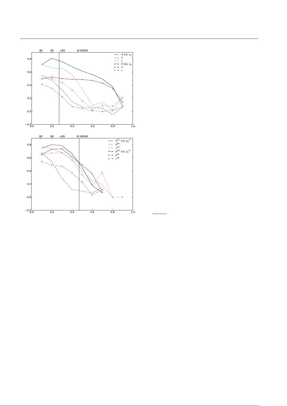
Climate Dynamics manuscript No. (will be inserted by the editor) How complex climate networks complement eigen techniques for the statistical analysis of climatological data Jonathan F . Donges · Irina Petr ova · Alexander Loew · Norbert Marwan · J ¨ urgen Kurths Receiv ed: date / Accepted: date Abstract Eigen techniques such as empirical orthogonal func- tion (EOF) or coupled pattern (CP) / maximum cov ariance analysis ha ve been frequently used for detecting patterns in multiv ariate climatological data sets. Recently , statisti- cal methods originating from the theory of complex net- works ha ve been employed for the very same purpose of spatio-temporal analysis. This climate network (CN) anal- ysis is usually based on the same set of similarity matrices as is used in classical EOF or CP analysis, e.g. , the corre- lation matrix of a single climatological ﬁeld or the cross- correlation matrix between two distinct climatological ﬁelds. In this study , formal relationships as well as conceptual dif- ferences between both eigen and network approaches are de- riv ed and illustrated using global precipitation, ev aporation and surface air temperature data sets. These results allow us to pinpoint that CN analysis can complement classical eigen techniques and pro vides additional information on the Jonathan F . Donges · Norbert Marwan · J ¨ urgen K urths Potsdam Institute for Climate Impact Research, P .O. Box 60 12 03, 14412 Potsdam, Germany E-mail: donges@pik-potsdam.de Jonathan F . Donges Stockholm Resilience Center, Stockholm University , Kr ¨ aftriket 2B, 114 19 Stockholm, Sweden Irina Petrov a Max-Planck-Institute for Meteorology , KlimaCampus, 20146 Ham- bur g, Germany Alexander Loe w Department of Geography , University of Munich (LMU), Luisen- str . 37, 80333 Munich, Germany J ¨ urgen K urths Department of Physics, Humboldt University , Newtonstr . 15, 12489 Berlin, Germany Institute for Complex Systems and Mathematical Biology , University of Aberdeen, Aberdeen AB243UE, United Kingdom Department of Control Theory , Nizhny Novgorod State Univ ersity , 603950 Nizhny No vgorod, Russia higher-order structure of statistical interrelationships in cli- matological data. Hence, CNs are a valuable supplement to the statistical toolbox of the climatologist, particularly for making sense out of very large data sets such as those gen- erated by satellite observations and climate model intercom- parison ex ercises. Keyw ords climate networks · empirical orthogonal functions · coupled patterns · maximum cov ariance analysis · climate data analysis 1 Introduction Climatologists hav e long been interested in studying corre- lations between climatological variables for gaining an un- derstanding of the Earth’ s climate system’ s large-scale dy- namics (Katz 2002). Pioneering work in this ﬁeld was done by Sir Gilbert T . W alker in the beginning of the 20th cen- tury while attempting to ﬁnd precursory patterns for Indian monsoon e vents using statistical methods (W alker 1910), which culminated in the discovery of the tropical W alker circulation and the Paciﬁc Southern Oscillation (a part of the El Ni ˜ no-Southern Oscillation known as ENSO). Later , new measurement devices as well as the rapid increase in av ailable computing power allowed to in vestigate statisti- cal interdependency structures of global or regional clima- tological ﬁelds x ( t ) = { x i ( t ) } N i =1 such as surface air tem- perature, pressure, or geopotential height (Fukuoka 1951; Lorenz 1956) (here, i is a spatial inde x, e.g . , labeling N me- teorological measurement stations or grid points in an ag- gregated data set, and t denotes time). Now adays, techniques of eigenanalysis such as empiri- cal orthogonal functions (EOFs) (Kutzbach 1967; W allace and Gutzler 1981; Hannachi et al 2007) and coupled pat- terns (CPs) (Bretherton et al 1992) are standard tools for ﬁnding spatial as well as temporal patterns in climatological 2 Donges, Petrov a et al. data (von Storch and Zwiers 2003). Their applications range from statistical predictions (Lorenz 1956; Brunet and V au- tard 1996; Repelli and Nobre 2004), over the deﬁnition of climate indices (Po wer et al 1999; Leroy and Wheeler 2008) to ev aluating the performance of climate model simulation runs (Handorf and Dethloff 2009, 2012). While numerous linear and nonlinear extensions have been proposed (Ghil and Malanotte-Rizzoli 1991; Ghil et al 2002), e.g., rotated or simpliﬁed EOFs (Hannachi et al 2007) and other methods of dimensionality reduction such as neural network-based nonlinear principal component analysis (PCA) (Hsieh 2004) or isometric feature mapping (ISOMAP) (T enenbaum et al 2000; G ´ amez et al 2004), classical EOF and CP analysis hav e remained among the most popular statistical techniques applied in climatology so far . In the last decade, complex network theory has been in- troduced as a po werful frame work for extracting informa- tion from lar ge volumes of high-dimensional data (New- man 2003; Boccaletti et al 2006; Newman 2010; Cohen and Havlin 2010) such as those generated by neurophysiolog- ical or biochemical measurements, quantitativ e social sci- ence as well as climatological observations and modeling campaigns. While EOFs, CPs, and related methods effec- tiv ely rely on a dimensionality reduction, network techniques allow to study the full complexity of the statistical interde- pendency structure within a multiv ariate data set. In these climate networks (CNs), which were ﬁrst introduced by Tso- nis and Roebber (2004); Tsonis et al (2006), nodes corre- spond to time series of climate variability at grid points or observational stations and links indicate a rele vant statistical association between two such time series. For quantifying statistical associations, linear cov ariance or Pearson correla- tion can be used analogously to EOF and CP analysis (Tso- nis and Roebber 2004; Tsonis and Swanson 2008; Y amasaki et al 2008), but nonlinear measures such as mutual informa- tion (Donges et al 2009a,b; Barreiro et al 2011) or trans- fer entropy (Runge et al 2012a) may be employed as well with care (Hlinka et al 2014). Among other applications, CNs have been used to uncover global impacts of El Ni ˜ no ev ents (Tsonis and Swanson 2008; Y amasaki et al 2008; Go- zolchiani et al 2011; Martin et al 2013; Radebach et al 2013), trace the ﬂo w of energy and matter in the surf ace air temper- ature ﬁeld (Donges et al 2009a), unra vel the complex dy- namics of the Indian summer monsoon (Malik et al 2012; Stolbov a et al 2014), detect community structure enabling statistical prediction of climate indices (Tsonis et al 2011; Steinhaeuser et al 2011, 2012) as well as intercomparisons between climate models and observ ations (Steinhaeuser and Tsonis in press; Feldhoff et al 2014), and study large-scale circulation patterns and prominent modes of variability in the atmosphere (Tsonis et al 2008; Donges et al 2011c; Ebert- Uphoff and Deng 2012a,b). Furthermore, CN analysis has recently been employed to improve forecasting of El Ni ˜ no episodes (Ludescher et al 2013, 2014), predict extreme pre- cipitation events over South America (Boers et al 2014a) and to deriv e early warning indicators for the collapse of the Atlantic meridional ov erturning circulation (Mheen et al 2013). Extending upon the majority of studies focussing on recent climate variability , the CN approach has also been applied to study late Holocene Asian summer monsoon dy- namics based on data from paleoclimate archives (Rehfeld et al 2013) The main aim of this contribution is to put the recent CN approach into context with standard eigenanalysis, since both classes of methods are often based on the same set of statistical similarity matrices. W e brieﬂy revie w both classes of techniques to establish a common notation. Formal re- lationships are then derived between empirical orthogonal functions or coupled patterns and frequently used CN mea- sures such as degree or cross-de gree, respecti vely . These re- lationships are illustrated empirically using global satellite observations of precipitation and ev aporation ﬁelds as well as surface air temperature reanalysis data. W e furthermore illustrate and ar gue in which settings higher-order CN mea- sures such as betweenness may contain information comple- menting classical eigenanalysis. For example, betweenness can be interpreted as approximating the ﬂow of energy and matter within a climatological ﬁeld and is particularly useful for identifying bottlenecks that may be particularly vulner- able to perturbations such as volcanic eruptions or anthro- pogenic inﬂuences (Donges et al 2009a, 2011c; Boers et al 2013; Molkenthin et al 2014a). Hence, by transferring in- sights and tools from complex network theory and comple x- ity science to climate research, CNs meet the need for no vel techniques of climate data analysis facing quickly increasing data volumes generated by growing observational networks and model intercomparison ex ercises like the coupled model intercomparison project (CMIP) (Meehl et al 2005; T aylor et al 2012). This article is structured as follo ws: After describing the data to be analyzed (Section 2), we introduce eigen (Sec- tion 3) and netw ork (Section 4) techniques for the statistical analysis of climatological data. Relationships between both approaches are formally derived and empirically demonstrated using observ ational climate data in Section 5. This leads us to pinpoint the added value of CN analysis (Section 6), be- fore concluding in Section 7. 2 Data Imperfect retriev al algorithms and data merging of atmo- spheric ﬁelds that are in volved in the generation of reanal- ysis data sets may cause uncertainties and lower quality of the ﬁnal product of data analysis. In order to obtain consis- tent and representativ e precipitation and ev aporation ﬁelds, in this study , the fully satellite-based HOAPS-3 (Hambur g How comple x climate networks complement eigen techniques for the statistical analysis of climatological data 3 Ocean Atmosphere Parameters and Fluxes from Satellite Data, http://www .hoaps.org, Andersson et al (2010b, 2011)) and combined HOAPS-3/ GPCC (Global Precipitation Climatol- ogy Center , http://www .gpcc.dwd.de, Andersson et al (2010a)) data sets are used. Regardless of the improved retrie val al- gorithms and high quality output product, the uniqueness of the HO APS data set consists in utilization of only one satel- lite data set for retriev al of both, e vaporation, and precipi- tation parameters. Originally available at the resolution of 0.5 degrees in latitude and longitude, monthly mean precip- itation ( x (t)) and ev aporation ( y (t)) anomaly ﬁelds ( 1992 – 2005 ) were resampled to T63 resolution ( ≈ 1 . 8 degrees) to reduce computational costs. Furthermore, areas with sea-ice cov erage were excluded from the set of raw time series. This results in N P = 13 , 834 and N E = 7 , 986 grid points (or network nodes) and M = 168 samples for each time series for the global precipitation and ev aporation data sets, respec- tiv ely . The smaller number of nodes in the ev aporation ﬁeld arises because the data are only av ailable over the oceans, but not ov er land. W e use the full global data sets for com- paring univ ariate techniques of climate data analysis, but for clarity restrict ourselves to the North Atlantic Ocean region for the multiv ariate methods. Additionally , to put our work into context with earlier work on CN analysis (Tsonis and Swanson 2008; Y amasaki et al 2008; Donges et al 2009a; Steinhaeuser et al 2012), we study global monthly av eraged surface air temperature (SA T) ﬁeld data covering the years 01/1948–12/2007 taken from the reanalysis I project provided by the National Cen- ter for En vironmental Prediction / National Center for At- mospheric Research (NCEP/NCAR, Kistler et al (2001)). This data set consists of N T = 10 , 224 grid points (network nodes) and M = 720 samples for each time series. 3 Eigenanalysis This section serves to introduce the mathematics of eige- nanalysis necessary for the deductions made belo w . Spe- ciﬁcally , standard EOF analysis of single climatological ﬁelds (e.g., the precipitation ﬁeld) as well as coupled patterns based on a singular value decomposition of the cross-correlation matrix (also termed maximum covariance analysis (MCA) in von Storch and Zwiers (2003)) for studying statistical re- lationships between two climatological ﬁelds (e.g., the pre- cipitation and ev aporation ﬁelds) are discussed. Of all the variants of eigenanalysis (Hannachi et al 2007), these two approaches appear to be the most frequently used and are also most closely related to CN and coupled CN analysis, respectiv ely , as will be elaborated on in Section 5. For fur- ther details, the reader is referred to Bretherton et al (1992); von Storch and Zwiers (2003) or Hannachi et al (2007). Note, that for consistency with the CN literature (see Section 4), we deﬁne EOFs (CPs) based on the correlation EOF analysis Network analysis Fig. 1 A schematic outline of the relationship between univ ariate EOF and climate netw ork analysis in the spirit of the diagrams in Bretherton et al (1992). The eigen decomposition (PCA) operation is represented by the square, the thresholding operation by the disc. All vectors are written in component form. (cross-correlation) instead of the cov ariance (cross-cov ariance) matrix. The results and conclusions presented in Sections 5 and 6 would not change qualitati vely if the covariance (cross- cov ariance) matrix would be used for both eigenanalysis and CN construction. 3.1 Empirical orthogonal function analysis Giv en a set of normalized time series x ( t ) = { x i ( t ) } N i =1 with zero mean and unit standard deviation, the correlation matrix C X = { C X ij } ij is deﬁned by C X ij = 1 M M X t =1 x i ( t ) x j ( t ) , (1) where M is the length (number of samples) of each time series. The aim of EOF analysis (also termed principal compo- nent analysis in the statistical literature (Preisendorfer and Mobley 1988)) is a dimensional reduction achiev ed by de- composing the data into linearly independent linear com- binations of the different variables that explain maximum variance (Hannachi et al 2007). The EOFs u k are obtained as solutions of the eigen v alue problem C X u k = λ k u k . (2) The k –th EOF u k is the eigen vector corresponding to the k – th lar gest eigen value λ k , where u ik denotes the i –th compo- nent of the k –th EOF (Fig. 1). The EOFs are sorted accord- ing to the ordering of their associated non-negati ve eigen- values λ k such that λ 1 ≥ λ 2 ≥ · · · ≥ λ R ( R is the rank of C X ). Hence, u 1 associated with the lar gest eigen value λ 1 is 4 Donges, Petrov a et al. V ariance explained (%) Fig. 2 Percentage of variance λ k / P R l =1 λ l explained by EOFs u k for the HO APS-3 / GPCC precipitation data set. Error bars were esti- mated using North’ s rule of thumb (North et al 1982). called the leading EOF of the underlying data set and rep- resents the one-dimensional projection of the data with the largest possible v ariance. The normalized data x i ( t ) can be decomposed as (Fig. 1) x i ( t ) = R X k =1 λ k a k ( t ) u ik , (3) where a k ( t ) is the t –th component of the k –th principal component a k (PC) (temporal pattern) associated with the k –th EOF u k (spatial pattern) with a k ( t ) = N X j =1 u kj x j ( t ) . (4) For many climatological data sets such as the precipitation and ev aporation ﬁelds studied here, most of the variance in the data x ( t ) can be explained by a small number of EOFs, i.e., the eigen values λ k decay quickly with increas- ing rank k (Fig. 2). Equation (3) sho ws that in this situation, only a fe w EOFs and PCs are needed to closely approximate the data which allows the dimensionality reduction of high- dimensional data sets. 3.2 Coupled pattern (maximum covariance) analysis Giv en two sets of normalized time series x ( t ) = { x i ( t ) } N X i =1 , and y ( t ) = { y j ( t ) } N Y j =1 the cr oss-corr elation matrix C X Y = { C X Y ij } ij is deﬁned by C X Y ij = 1 M M X t =1 x i ( t ) y j ( t ) , (5) Coupled pattern analysis Network analysis Fig. 3 A schematic outline of the relationship between coupled pat- tern (maximum covariance) and coupled climate network analysis in the spirit of the diagrams in Bretherton et al (1992). The singular value decomposition (SVD) operation is represented by the triangle, the thresholding operation by the disc. All vectors are written in com- ponent form. Cross-covariance explained (%) Fig. 4 Percentage of squared covariance σ 2 k / P R l =1 σ 2 l between HO APS-3 / GPCC precipitation ( X ) and HOAPS-3 ev aporation ( Y ) data sets over the North Atlantic region (see Fig. 7) that is explained by pairs of coupled patterns p X k , p Y k . Most of the data sets’ cross- cov ariance is captured by a small number of modes with the largest singular values σ k . Error bars were estimated using North’ s rule of thumb (North et al 1982). where M is the length (number of samples) of each time series. R in the following denotes the rank of C X Y . Maximum cov ariance analysis identiﬁes spatially ortho- normal pairs of coupled patterns p X k = { p X ik } N X i =1 , p Y k = { p Y j k } N Y j =1 that explain as much as possible of the temporal How comple x climate networks complement eigen techniques for the statistical analysis of climatological data 5 cov ariance between the two ﬁelds x ( t ) and y ( t ) (Brether- ton et al 1992; von Storch and Zwiers 2003). The coupled patterns can be found by solving the system of equations ( C X Y ) T p X k = σ k p Y k C X Y p Y k = σ k p X k (6) by means of a singular value decomposition of C X Y (Fig. 3). Here, the p X k are an orthonormal set of R vectors called left singular vectors , the p Y k are an orthonormal set of R vectors called right singular vectors , and the σ k are non- negati ve numbers called singular values , ordered such that σ 1 ≥ σ 2 ≥ · · · ≥ σ R . Here, R denotes the rank of C X Y . The total squared cov ariance explained by a certain pair of patterns p X k , p Y k is σ 2 k . Therefore, the leading coupled pat- terns p X 1 , p Y 1 explain the lar gest fraction of squared covari- ance between the two ﬁelds of interest. In our example, tak- ing into account only a few pairs of coupled patterns with the largest σ k already explains most of the cov ariance between the precipitation and ev aporation ﬁelds (Fig. 4). The ﬁelds x ( t ) , y ( t ) can be expanded in terms of the coupled patterns as x i ( t ) = R X k =1 a X k ( t ) p X ik , (7) y i ( t ) = R X k =1 a Y k ( t ) p Y ik . (8) The expansion coef ﬁcients are obtained by projecting a X k ( t ) = R X i =1 p X ik x i ( t ) , (9) a Y k ( t ) = R X i =1 p Y ik y i ( t ) . (10) 4 Network techniques Complex network analysis offers a general framework for studying the structure of associations (links) between ob- jects (nodes) that are of interest in many disciplines. T yp- ical examples include the internet or world wide web in computer science, road networks and power grids in engi- neering, food webs in biology or social networks in sociol- ogy (Newman 2003; Boccaletti et al 2006; Ne wman 2010; Cohen and Havlin 2010). It has become popular recently in sev eral ﬁelds of science to apply the wealth of concepts and measures from complex network theory for the analysis of data that is ev en not giv en explicitly in network form. In network-based data analysis, a data set at hand, e.g . , con- sisting of time series such as electroencephalogram, climate records, or spatiotemporal point ev ents such as earthquake aftershock swarms, ﬁrst has to be transformed to a network representation by means of a suitable algorithm or mathe- matical mapping. The resulting networks are referred to as functional networks to distinguish them from structur al net- works that are deriv ed from systems with a more obvious graph structure, e.g . , social networks or power grids. Ex- amples of functional networks include gene regulatory net- works in biology (Hempel et al 2011), functional brain net- works in neuroscience (Bullmore and Sporns 2009), CNs in climatology (Donges et al 2009a,b, 2011c), or networks of earthquake aftershocks in seismology (Da vidsen et al 2008). Forming a distinct class of methods, techniques for the network- based analysis of single or multiple time series such as recur- rence networks (Xu et al 2008; Marwan et al 2009; Donner et al 2010) and visibility graphs (Lacasa et al 2008) hav e recently been studied intensiv ely with a focus on (paleo- )climatological applications (Donges et al 2011a,b; Hirata et al 2011; Donner and Donges 2012; Feldhoff et al 2012). The ﬁrst functional network analysis of ﬁelds of climato- logical time series x ( t ) was presented by Tsonis and Roeb- ber (2004), introducing the term climate network 1 . Climate network analysis offers novel insights by transferring the toolbox of measures and algorithms from complex network theory to the study of climate system dynamics. Climate net- works are simple graphs (i.e., there are no self-loops and at most one link between each pair of nodes) consisting of N spatially embedded nodes i that correspond to time series x i ( t ) representing observations, reanalyses, or simulations of climatological variables at ﬁxed measurement stations, grid cells, or certain predeﬁned regions. Links { i, j } repre- sent particularly strong or signiﬁcant statistical interdepen- dencies between two climate time series x i ( t ) , x j ( t ) , where usually a ﬁltering procedure is applied ﬁrst to reduce the ef- fects of the annual cycle (Donner et al 2008). Put dif ferently , for a pairwise measure of statistical asso- ciation S ij such as Pearson correlation (Tsonis and Roebber 2004; Tsonis et al 2006), mutual information (Donges et al 2009b,a; Palu ˇ s et al 2011), transfer entropy (Runge et al 2012a), or ev ent synchronization (Malik et al 2012; Boers et al 2013; Stolbov a et al 2014; Boers et al 2014b), a CN’ s adjacency matrix is gi ven by A ij = ( Θ ( S ij − T ij ) if i 6 = j, 0 otherwise , (11) 1 Note that the term climate network is also used in distinct contexts that are unrelated to graph theory or data analysis, e.g. , for describ- ing collections of climatological/weather observation stations like the Gr eenland climate network (Stef fen and Box 2001) or associations of political organizations dealing with anthropogenic climate change such as the Climate Network Eur ope (Raustiala 2001). 6 Donges, Petrov a et al. where Θ ( · ) is the Heaviside function, T ij denotes a thresh- old parameter , and A ii = 0 is set for all nodes i to ex- clude self-loops. Usually , the threshold is ﬁxed globally , i.e. , T ij = T for all node pairs ( i, j ) . Howe ver , T ij may also be set for each pair individually to only include links with val- ues of S ij exceeding a prescribed signiﬁcance lev el, e.g., determined from a statistical test using surrogate time se- ries (Palu ˇ s et al 2011). In most studies, symmetric measures of statistical interdependency S ij = S j i hav e been consid- ered, leading to undirected CNs. Ho wev er , Gozolchiani et al (2011), Malik et al (2012) and Boers et al (2014b) exploited asymmetries in the cross-correlation function as well as in a measure of ev ent synchronization to reconstruct directed CNs. In the following, univ ariate and coupled CNs are intro- duced for studying the statistical interdependency structure within single ﬁelds as well as between two ﬁelds, respec- tiv ely , together with graph-theoretical measures that are typ- ically used for their quantiﬁcation. For consistency with eige- nanalysis (see Section 3), we restrict ourselves to linear Pear- son correlation at zero lag as the measure of statistical asso- ciation, i.e. , S ij = | C ij | . 4.1 Univ ariate climate networks Giv en a climatological ﬁeld x ( t ) , the adjacency matrix A = { A ij } ij of the associated climate network is given by A ij = Θ (   C X ij   − T ) − δ ij (12) with a prescribed global threshold 0 ≤ T ≤ 1 , where δ ij denotes Kronecker’ s delta (see Eq. (1) for the deﬁnition of C X ij ). The absolute value of Pearson correlation   C X ij   is com- monly used, typically because ne gativ e correlations are con- sidered equally important as positiv e ones (Tsonis and Roeb- ber 2004). Among others, uni variate CNs ha ve been studied by Tsonis et al (2006); Tsonis and Swanson (2008); Tsonis et al (2008); Y amasaki et al (2008); Gozolchiani et al (2008); Y amasaki et al (2009); Donges et al (2009a,b); Tsonis et al (2011); Berezin et al (2012); Gozolchiani et al (2011); Guez et al (2012); Palu ˇ s et al (2011); Donges et al (2011c); T omin- ski et al (2011); Zou et al (2011); Malik et al (2012); Rhein- walt et al (2012); Rehfeld et al (2013). The de gr ee k i is the most frequently applied measure for studying CNs. It giv es the number of network neighbors for each node i and is deﬁned as k i = N X j =1 A ij = N X j =1 Θ (   C X ij   − T ) − 1 . (13) Maxima in the spatial pattern k with v alues of the degree that are much larger than av erage are referred to as super- nodes or hubs (Tsonis and Roebber 2004; Tsonis et al 2006). These super-nodes indicate regions in the underlying ﬁeld that are particularly strongly correlated to many other parts of the globe which are typically related to teleconnection patterns (Tsonis et al 2008). For example, in the HOAPS-3 / GPCC precipitation data the most strongly connected re- gion in the tropical Paciﬁc (Fig. 5B) corresponds to the El Ni ˜ no-Southern Oscillation that is known to display global teleconnections (Ropele wski and Halpert 1987; Halpert and Ropelewski 1992; Tsonis et al 2008). Path-based centrality measures from network theory re- veal higher-order patterns in the statistical interdependency structure of a climatological ﬁeld (Donges et al 2009a,b; Palu ˇ s et al 2011). High-order , in this context, refers to struc- tures such as paths or network motifs that consist of two or more links, in contrast to the degree that is restricted to counting pairwise relationships between nodes. In this study , shortest-path closeness and betweenness are consid- ered. Closeness centrality c = { c i } N i =1 (CC) measures the in verse mean network distance of node i to all other nodes via shortest paths and is deﬁned as c i = N − 1 P N j =1 l ij , (14) where l ij denotes the length of a shortest (or geodesic) path connecting nodes i and j , i.e. , the smallest number of links that are passed when trav eling from i to j in the CN. In contrast, betweenness b = { b i } N i =1 (BC) counts the rela- tiv e number of shortest paths connecting any pair of nodes j, k that include node i and is deﬁned as b i = N X j =1 N X k =1 n j k ( i ) n j k . (15) Here, n j k denotes the total number of shortest paths between j, k . n j k ( i ) giv es the size of the subset of these paths that in- clude i . CC and BC ha ve been applied for comparing differ - ent types of CNs (Donges et al 2009b), re vealing a backbone of energy ﬂow in the surface air temperature ﬁeld (Donges et al 2009a), unraveling the complex dynamics of the pre- cipitation ﬁeld during the Indian summer monsoon (Malik et al 2012), and studying the signatures of El Ni ˜ no and La Ni ˜ na ev ents (Palu ˇ s et al 2011). See Section 6 for a more in depth discussion of the interpretation of these CN measures. 4.2 Coupled climate networks One option for condensing information from more than one climatological observable in a CN is to deﬁne links based on statistical interdependencies between multiv ariate time series describing the dynamics of multiple observ ables rec- orded at the same locations/nodes. For example, Steinhaeuser How comple x climate networks complement eigen techniques for the statistical analysis of climatological data 7 Leading EOF u 1 Percentage of variance explained by u 1 Fig. 5 Maps of (A) ﬁrst EOF u 1 , (B) climate network degree ﬁeld k , and (C) local percentage of variance explained by ﬁrst EOF u 1 , 100 × Corr ( x i ( t ) , a 1 ( t )) 2 (homogeneous correlation map, see Bj ¨ ornsson and V enegas (1997)), for the global HOAPS-3 / GPCC precipitation data set. The climate network construction threshold T = 0 . 27 was chosen to yield a link density of ρ = 0 . 01 (Eq. (25)). Note the sim- ilarity in the patterns displayed in panels (A)–(C) that is explained in Section 5. V Y V X E XY E XX E YY Fig. 6 A coupled climate network as it is constructed in this work, where V X and V Y denote the set of nodes in the subnetworks corre- sponding to grid points in data sets x ( t ) and y ( t ) , respecti vely . E X X and E Y Y are sets of internal links within the subnetworks describing statistical relationships within each climatological ﬁeld, while E X Y contains information on their mutual statistical interdependencies. Fig- ure is adapted from (Donges et al 2011c). et al (2010) analyzed a CN constructed from surf ace air tem- perature, pressure, relative humidity , and precipitable water to extract regions of related climate variability . In contrast to this multiv ariate approach, coupled CNs are designed to rep- resent statistical dependencies within and between two cli- matological ﬁelds x ( t ) = { x i ( t ) } N X i =1 , y ( t ) = { y j ( t ) } N Y j =1 or within and between different regions (Donges et al 2011c). For this purpose, all time series from each of the in volv ed climatological ﬁelds are associated to N X + N Y nodes in the resulting network (Fig. 6). A coupled CN is deﬁned by its adjacency matrix A that is obtained by thresholding the correlation matrix C of the concatenated ﬁelds x ( t ) , y ( t ) , analogously to Eq. (12). Decomposing C as C =  C X C X Y ( C X Y ) T C Y  (16) suggests to view coupled CNs as networks of networks or multilayer networks (Zhou et al 2006; Buldyrev et al 2010; Gao et al 2011; Boccaletti et al 2014), where subnetworks (network layers) G X = ( V X , E X X ) and G Y = ( V Y , E Y Y ) are the induced subgraphs of the sets of nodes V X , V Y be- longing to data sets x ( t ) , y ( t ) , respectively (Fig. 6). While the edge sets E X X , E Y Y describe the ﬁelds’ internal corre- lation structure based on the correlation matrices C X , C Y , the set of cross-edges E X Y captures dependencies between both ﬁelds and is based on the cross-correlation matrix C X Y (Fig. 3). Coupled CNs have been applied for studying the Earth’ s atmosphere’ s general circulation structure (Donges et al 2011c), processes linking climate variability in the North Atlantic and North Paciﬁc regions via the Arctic (W ieder- mann et al 2013, in prep.), global atmosphere-ocean inter- actions (Feng et al 2012). Also, the coupled CN approach underlies the method developed in Ludescher et al (2013, 2014) for forecasting El Ni ˜ no ev ents. The statistical interdependency structure between ﬁelds x ( t ) , y ( t ) can be quantiﬁed with a set of graph-theoretical 8 Donges, Petrov a et al. Fig. 7 Maps of leading pair of coupled patterns (A) p X 1 and (B) p Y 1 , coupled climate network cross-degree ﬁelds (C) k X Y and (D) k Y X , and percentage of cross-cov ariance explained by ﬁrst pair of coupled patterns (E) p Y 1 , 100 × Corr ( x i ( t ) , a Y 1 ( t )) 2 , and (F) p X 1 , 100 × Corr ( y i ( t ) , a X 1 ( t )) 2 (heterogeneous correlation maps, see Bj ¨ ornsson and V enegas (1997)), for the HO APS-3 / GPCC precipitation ( X ) and HO APS-3 e vaporation ( Y ) data sets over the North Atlantic. For constructing the coupled climate network, a threshold T = 0 . 47 was chosen to yield a cross-link density of ρ X Y = 0 . 01 (Eq. (31)) resulting in internal link densities ρ X = 0 . 01 and ρ Y = 0 . 06 (Donges et al 2011c). How comple x climate networks complement eigen techniques for the statistical analysis of climatological data 9 measures dev eloped for inv estigating the topology of net- works of interacting networks (Donges et al 2011c). The cr oss-degr ee k X Y = { k X Y i } N X i =1 is the number of neighbors of node i ∈ V X in subnetwork G Y : k X Y i = X j ∈ V Y A ij = N Y X j =1 A X Y ij = N Y X j =1 Θ ( | C X Y ij | − T ) . (17) Analogously , the cross-degree k Y X = { k Y X j } N Y j =1 is given by k Y X j = X i ∈ V X A ij = N X X i =1 A X Y ij = N X X i =1 Θ ( | C X Y ij | − T ) . (18) Similarly to degree in univ ariate climate networks, re gions i in ﬁeld x ( t ) with a large cross-degree k X Y i are considered to be strongly dynamically interrelated with many locations in ﬁeld y ( t ) and vice versa. For the precipitation and ev ap- oration data sets (Fig. 7C,D), such regions with high cross- connectivity correspond to major covariability areas of ev ap- oration and precipitation ﬁelds driv en by the North-Atlantic Oscillation (N A O) (Andersson et al 2010b; Petrova 2012). Furthermore, analogously to univ ariate climate networks, generalizations of path-based measures for network of net- works can be deri ved (Donges et al 2011c). Here, cross- closeness and cross-betweenness are considered. Cr oss-close- ness c X Y = { c X Y i } N X i =1 (cross-CC) measures the in verse mean network distance of node i ∈ V X to all nodes j ∈ V Y via shortest paths and is deﬁned as c X Y i = N X + N Y − 1 P j ∈ V Y l ij . (19) Cr oss-betweenness b X Y = { b X Y i } N X i =1 (cross-BC) counts the relative number of shortest paths connecting any pair of nodes j ∈ V X , k ∈ V Y that include node i ∈ V X and is deﬁned as b X Y i = X j ∈ V X X k ∈ V Y n j k ( i ) n j k . (20) For nodes j in ﬁeld y ( t ) , the measures c Y X = { c Y X j } N Y j =1 and b Y X = { b Y X j } N Y j =1 are obtained from analogous ex- pressions following Donges et al (2011c). Interpretations of coupled CN measures will be discussed in Section 6. 5 Relationships between eigen and climate network analysis Comparing the results of eigen and CN analysis, notable similarities become apparent, e.g., in the leading EOF u 1 and CN degree k for the HO APS-3 / GPCC precipitation data (Fig. 5). Analogous relations are observed when in- specting leading coupled patterns and coupled CN cross- degree for HOAPS-3 / GPCC precipitation and HOAPS- 3 ev aporation data (Fig. 7). T o explain these similarities, in this section, formal relationships between patterns from eigen and CN analysis are derived and illustrated empiri- cally for global precipitation and ev aporation data sets. Re- lations between single ﬁeld (EOFs and univ ariate CN mea- sures, Section 5.1) as well as multiple ﬁeld patterns (cou- pled patterns and coupled CN measures, Section 5.2), and temporal patterns are discussed. Note that similar relation- ships hold when both eigen and network analysis are based on a type of symmetric similarity matrix that is different from linear correlation at zero lag, e.g. , considering mutual information (Donges et al 2009a,b) or the ISOMAP algo- rithm (T enenbaum et al 2000; G ´ amez et al 2004). 5.1 Single ﬁeld patterns As the correlation matrix C X is symmetric and, hence, di- agonalizable, it can be decomposed with respect to its eigen- system such that C X ij = R X k =1 u ik λ k u j k . (21) If the leading EOF u 1 explains a large fraction of the total variance, i.e . , if λ 1  λ 2 , then C X ij can be approximated as C X ij ≈ λ 1 u i 1 u j 1 . (22) Inserting this expression into the deﬁnition of CN degree (Eq. (13)) yields k i ≈ N X j =1 Θ ( λ 1 | u i 1 u j 1 | − T ) − 1 . (23) This approximation explains the empirically observed sim- ilarity between degree k and the leading EOF u 1 (compare Fig. 5, panels A and B, for the precipitation data set) in the following way: All nodes j with | u j 1 | > T λ 1 | u i 1 | contribute to the degree k i at node i , hence, a larger | u i 1 | typically leads to more positive contributions to the sum in Eq. (23) and, therefore, to a larger degree k i . Consequently , CN degree k 10 Donges, Petrov a et al. A Threshold T Pearson correlation Threshold T Pearson correlation B Fig. 8 Linear correlations between spatial patterns from eigen and network techniques for climate data analysis. Pearson correlation be- tween (A) the absolute values of the ﬁrst two EOFs | u 1 | , | u 2 | and CN measures degree k , closeness c and betweenness b for HOAPS- 3 / GPCC precipitation data as well as (B) the ﬁrst coupled pat- terns p X 1 , p Y 1 and coupled CN measures cross-degree k X Y , k Y X , cross-closeness c X Y , c Y X , and cross-betweenness b X Y , b Y X for HO APS-3 / GPCC precipitation (X) and HOAPS-3 ev aporation data. In both panels, correlations are displayed for varying network construc- tion threshold T , where the corresponding p -value according to the Student’ s t -test is given on the upper horizontal axis. V ertical lines in panels (A) and (B) indicate the thresholds used in Figs. 5 and 7, re- spectiv ely . and the vector of absolute values of the leading EOF’ s ele- ments | u 1 | are expected to be positi vely correlated. For the global precipitation data set, a large positiv e cor - relation between k and | u 1 | is indeed detected for interme- diate thresholds T of the order where CNs are typically con- structed (Donges et al 2009b), while for smaller and larger thresholds, the correlation decreases (Fig. 8A). The latter is expected, since both for T → 0 (fully connected network) and T → 1 (network dev oid of links), the CN contains no information about the climatological ﬁeld anymore and the degree ﬁeld is constant with k i → N − 1 and k i → 0 for all nodes i , respectiv ely . Hence, maximum pattern correspon- dence is e xpected for intermediate thresholds T (for these as well as computational reasons, results for T = 0 and T = 1 are not included in Fig. 8). Notably , selecting T as maximiz- ing the correlation between degree k and the leading EOF | u 1 | could provide a criterion for an informed choice of the threshold T . Such a choice would approximate a situation where the information that the CN contains on linear statis- tical interdependencies in the ﬁeld of interest is maximized. Further work is needed to dev elop more suitable criteria for deﬁning binary CNs with maximum information content. Furthermore and as expected, the correlation between de- gree k and the second EOF | u 2 | is mostly smaller than that between degree and leading EOF (Fig. 8A). Using the full eigen-decomposition of C X , an exact re- lationship between the degree k and all EOFs u k together with their associated eigen v alues λ k can be deriv ed as k i = N X j =1 Θ      R X k =1 u ik λ k u j k      − T ! − 1 . (24) Using this expression, the scalar link density ρ = h k i i N i =1 N − 1 (25) can likewise be expanded or approximated, where h·i de- notes the arithmetic mean. Similarly , a relationship between area-weighted EOFs (Hannachi et al 2007), the area-weighted degree (Heitzig et al 2012) (also called area weighted con- nectivity (Tsonis et al 2006)) and all other network measures directly expressible in terms of the adjacenc y matrix A ij can be deriv ed. 5.2 Coupled patterns The cross-correlation matrix C X Y can be decomposed in terms of singular values and coupled patterns as (Fig. 3) C X Y ij = R X k =1 σ k p X ik p Y j k . (26) The relationship between cross-degree k X Y , k Y X and cou- pled patterns p X k , p Y k can then be deriv ed as abov e: How comple x climate networks complement eigen techniques for the statistical analysis of climatological data 11 k X Y i = N Y X j =1 Θ      R X k =1 σ k p X ik p Y j k      − T ! (27) ≈ N Y X j =1 Θ  σ 1   p X i 1 p Y j 1   − T  , (28) k Y X j = N X X i =1 Θ      R X k =1 σ k p X ik p Y j k      − T ! (29) ≈ N X X i =1 Θ  σ 1   p X i 1 p Y j 1   − T  . (30) The approximations hold for the maximum singular value fulﬁlling σ 1  σ 2 ≥ · · · ≥ σ R . R is the rank of the cross- correlation matrix C X Y . By a similar argument as gi ven abov e this shows that k X Y and | p X 1 | ( k Y X and | p Y 1 | ) are expected to be positiv ely correlated which is consistent with our results regarding the interdependenc y structure between precipitation and ev aporation ﬁelds. While in our example, the correspondence between the resulting patterns is some- what less pronounced than in the single-ﬁeld setting (Fig. 8B), still regions with a strongly negati ve loading in the leading coupled patterns p X 1 and p Y 1 appear as super nodal struc- tures in the cross-degree ﬁelds (Fig. 7). When studying vary- ing network construction thresholds T , as in the case of single-ﬁeld patterns, the correlation between the absolute values of the leading pair of coupled patterns and cross- degree ﬁelds is maximum for intermediate T and decreases for T → 0 and T → 1 (Fig. 8B). Also, consistently with Eqs. (27) and (29), the correlation between the second pair of coupled patterns and cross-degree ﬁelds is always smaller than that observed for the leading pair of coupled patterns (results not shown). The scalar cross-link densities (Donges et al 2011c) ρ X Y =  k X Y i  N X i =1 N Y ρ Y X =  k Y X j  N Y j =1 N X (31) can also be e xpanded and approximated in terms of CPs and singular values using the above expressions. Analogously , area-weighted coupled patterns (von Storch and Zwiers 2003) are related to the area-weighted cross-degree introduced by Feng et al (2012) and W iedermann et al (2013). 5.3 T emporal patterns In EOF analysis, temporal patterns (principal components) a k ( t ) describing the e volution of their associated spatial pat- terns u k are easily obtained by projecting the data x ( t ) onto the latter patterns u k (Eq. (4)). Analogously , the same holds for multiv ariate extensions such as coupled pattern analy- sis (Bretherton et al 1992; von Storch and Zwiers 2003), see Section 3. In CN analysis, ho wev er , the temporal ev o- lution of spatial network measure patterns such as the de- gree k or betweenness b cannot be directly obtained from the adjacency matrix A and x ( t ) . T o allow the study of non-stationarities i n the statistical interdependence structure of climatological ﬁelds, sev eral authors ha ve inv estigated the ev olving local ( e.g . , k ( t ) or b (t)) and global properties of CNs A ( t ) constructed from temporal windows sliding ov er the time series data (Gozolchiani et al 2008; Y amasaki et al 2008, 2009; Gozolchiani et al 2011; Guez et al 2012; Berezin et al 2012; Carpi et al 2012; Martin et al 2013; Rade- bach et al 2013; Ludescher et al 2013, 2014). A similar strat- egy could be applied to coupled CN analysis. It should be noted that unlike in the abov e sections, no direct relationship can be deriv ed linking temporal patterns from eigen and network analysis. The reason for this is tw o- fold. First, temporal patterns a k ( t ) of standard EOF analysis are based on the full data set x ( t ) , while the ev olving spa- tial network patterns are computed from subsets (deﬁned by temporal windo ws) of x ( t ) . Second, since temporal patterns a k ( t ) of eigenanalysis are merely scalar prefactors in the expansion Eq. (3) (see Figs. 1 and 3), the spatial EOF pat- terns u k are time-independent, whereas evolving CN mea- sures such as k ( t ) can vary independently at ev ery location i . Hence, in contrast to standard EOF patterns, the spatial pat- terns in the network properties derived from e volving CNs are explicitly time-dependent. The latter case is analogous to extended EOF analysis, where standard EOF analysis is applied in a sliding-window mode as well (Fraedrich et al 1997). 6 Discussion The relationships derived in the previous section provide guidance on deciding how and in which applications CN analysis can be expected to yield information that is com- plementary to the results of eigenanalysis. Particularly , we will focus on a discussion and climatological interpretation of single ﬁeld and coupled patterns deriv ed from precipita- tion and ev aporation data (Section 6.1) and relate this to a study of single ﬁeld patterns for global surface air temper- ature data (Section 6.2). Based on these insights, we point out some methodological as well as practical potentials of CN analysis of climatological ﬁelds (Section 6.3). 6.1 Precipitation and ev aporation data For the HOAPS-3 / GPCC precipitation and HO APS-3 ev ap- oration data sets, pronounced similarities between the fea- 12 Donges, Petrov a et al. tures observ ed in the degree or cross-degree ﬁelds and those in the leading EOF or coupled patterns that are deri ved from the same data hav e been described and explained mathe- matically (Section 5). More speciﬁcally , activ e regions dis- playing strong correlations with many other locations, and, hence, a large degree or cross-degree (termed super-nodes in the context of CN analysis (Tsonis and Roebber 2004; Tsonis et al 2006; Barreiro et al 2011)) correspond to re- gions with large positiv e or neg ativ e loading in the lead- ing EOF or coupled patterns. For example, this can be ob- served for the equatorial Paciﬁc in the precipitation data (Fig. 5A,B). The spatial similarity between the amplitude of the leading EOF and CN degree ﬁeld re veals the well- known ENSO variability pattern (Ropelewski and Halpert 1987). Particularly , the patterns in the explained variance fraction (Fig. 5C) closely resemble high connectivity areas of the CN resembling most prominent ENSO teleconnec- tions (Andersson et al 2010b; Halpert and Ropelewski 1992; Ropelewski and Halpert 1987). Additional dipole informa- tion described by the EOF is typically preserved by neigh- bors of the network’ s major super-nodes (not shown here, see Petrov a (2012) and Kaw ale et al (2013)). Considering the biv ariate analysis of precipitation and ev aporation data ov er North Atlantic (Fig. 7), regions with a strongly negati ve loading in the leading pair of coupled patterns appear as super nodal structures in the cross-degree ﬁelds obtained from coupled CN analysis. Areas with a high fraction of explained cross-covariance (Fig. 7E,F) well cor- respond to the coupled network topology as indicated by the cross-degree ﬁelds (Fig. 7C,D) and all together depict major covariability areas of ev aporation and precipitation driv en by the NA O. The cross-degree ﬁeld k X Y (Fig. 7C), displaying the number of strong correlations between pre- cipitation variability at a certain location with ev aporation dynamics at all other grid points, reveals teleconnections as- sociated to the N A O ov er the southern tip of Greenland as well as a positiv e NA O signal over Portugal and a negati ve N A O signal over Norway (Andersson et al 2010b). In turn, the cross-degree ﬁeld k Y X (Fig. 7D), showing the number of strong correlations between ev aporation dynamics at one point and precipitation variability at all other locations, is only av ailable over the ocean and follows the covariance structure of the main ev aporation determinant parameters with N A O (Cayan 1992; Marshall et al 2001). Beyond the frequently studied degree k , complex net- work theory provides a wealth of additional measures that can be used to study higher-order properties of the statisti- cal interdependency structure within and between climato- logical ﬁelds. For example, the mentioned measures based on the properties of shortest paths in (coupled) CNs such as (cross-) closeness c ( c X Y , c Y X ) and (cross-) betweenness b ( b X Y , b Y X ) (Fig. 9) hav e been argued to gi ve insights on the local speed of propagation as well as the preferred Fig. 9 Maps of (A) leading EOF u 1 , (B) closeness ﬁeld c , and (C) be- tweenness ﬁeld b for the global HOAPS-3 / GPCC precipitation cli- mate netw ork. The network construction threshold T = 0 . 27 was cho- sen to yield a link density of ρ = 0 . 01 . pathways for the spread of perturbations within or between the studied ﬁelds, respectiv ely (Donges et al 2009a,b, 2011c; Malik et al 2012; Molkenthin et al 2014a). In this way , CN analysis has the potential to unv eil information on climate dynamics from climatological ﬁeld data that conceptually supplements the results of eigenanalysis. Focussing on the precipitation data to further in vestigate this aspect, we ﬁnd that the correlation of CC and BC to the ﬁrst two EOFs obtained from the data are systematically and How comple x climate networks complement eigen techniques for the statistical analysis of climatological data 13 V ariance explained (%) Fig. 10 Percentage of variance λ k / P R l =1 λ l explained by EOFs u k for the NCEP/NCAR surface air temperature data set. Error bars were estimated using North’ s rule of thumb (North et al 1982). signiﬁcantly smaller than that between the degree ﬁeld and the same EOFs (Fig. 8A). Similarly , in the bi variate case, the correlations of cross-CC and cross-BC with the leading coupled pattern are considerably smaller than those between the latter and cross-degree for most thresholds T (Fig. 8B). Howe ver , for the HOAPS-3 / GPCC precipitation data, the patterns observed in the leading EOF resemble those found in the CC and BC ﬁelds (Fig. 9) as well as those in the de- gree ﬁeld (Fig. 5). These results can be explained from a net- work point of view by considering that precipitation ﬁelds are typically only correlated on short spatial scales and dis- play a smaller degree of spatial coherency when compared to other atmospheric variables such as pressure or temper - ature (Feldhoff et al 2014). In turn, this leads to a larger degree of randomness in the structure of CNs constructed from this data. In random networks, correlations between centrality measures such as degree, closeness and between- ness arise (Boccaletti et al 2006). In other words, spatially incoherent climatological ﬁelds can giv e rise to CNs with a notable degree of disorder in the placement of links be- tween dif ferent nodes which induces correlations between network centrality measures. For the precipitation data set at hand, the ﬁrst eigen value separates from the remaining spectrum (Fig. 2) leading to a pronounced correlation be- tween the leading EOF u 1 and the degree ﬁeld (see Eq. 23), and, hence, to correlations between u 1 and CC, BC. 6.2 Surface air temperature data Next, we in vestigate the NCEP/NCAR reanalysis I surface air temperature (SA T) ﬁeld as another frequently studied data set. The properties of this data are complementary to those of the precipitation ﬁeld discussed abov e in two as- pects: (i) for the SA T data, the leading two EOFs explain approximately the same amount of v ariance (Fig. 10), while the leading eigen value separates more markedly from the re- mainder of the spectrum in the case of the precipitation data (Fig. 2), and, (ii) the SA T ﬁeld is kno wn to display a stronger degree of spatial coherency than the precipitation ﬁeld. In the light of the discussion in Section 6.1, these two prop- erties are reﬂected when comparing the leading three EOFs and network properties for the SA T data set (Fig. 11). Firstly , the degree ﬁeld resembles the leading EOF less than in case of precipitation data (Fig. 11A,D), which is expected due to the weaker separation of the leading eigenv alues (Sec- tion 5.1 and Eq. 23). Consistently , the degree ﬁeld displays an even less pronounced similarity to the second and third EOFs (Fig. 11B,C,D). While the patterns found in the CC ﬁeld (Fig. 11E) still partly resembles those in the degree ﬁeld (Fig. 11D) as well as those in the leading two EOFs (Fig. 11A,B), the BC ﬁeld displays markedly distinct fea- tures (Fig. 11F). Only in a few regions, these structures of high betweenness appear to coincide with patterns of large EOF loadings, e.g., high betweenness structures found along the W est coasts of North and South America correspond to large positiv e loadings in the second and third EOFs, respec- tiv ely . The observed linear wav e-like structures of large BC in the SA T ﬁeld hav e been interpreted as signatures of the transport of temperature anomalies in strong surface ocean currents (Donges et al 2009a,b). For example, the large be- tweenness structures resemble strong western boundary cur - rents such as the Kuroshio of the east coast of Japan or Eastern boundary currents such the Canary current off the African west coast. It should be noted that while some of the structures in the BC ﬁeld such as the one resembling the North Atlantic’ s subtropical gyre appear blurred, the loga- rithmic color scale in Fig. 11F implies that ev en small changes in color correspond to exponentially large changes in BC. This interpretation of high betweenness structures in CNs constructed based on Pearson correlation as advecti ve struc- tures such as strong currents is supported by recent analyt- ical studies that are based on well-known ﬂuid dynamical model systems (Molk enthin et al 2014a,b). Further evidence that is also consistent with this interpretation of between- ness was found in a study of vertical interactions in the at- mospheric geopotential height ﬁeld, where regions of large cross-BC in the Arctic suggest that vertical air induced by the Arctic vortex is important for mediating the propaga- tion of wind ﬁeld anomalies between dif ferent isobaric sur- faces (Donges et al 2011c). Also, Boers et al (2013) employ BC and further network measures for precipitation data o ver South America to highlight the importance of atmospheric structures such as the South American low lev el jet for the propagation of extreme rainfall events, speciﬁcally over long distances. 14 Donges, Petrov a et al. Fig. 11 Maps of (A,B,C) the leading three EOFs u 1 , u 2 , u 3 , (D) normalized de gree ﬁeld k / ( N − 1) , (E) closeness ﬁeld c , and (F) betweenness ﬁeld b for the global NCEP/NCAR surface air temperature climate network. The network construction threshold T = 0 . 67 was chosen to yield a link density of ρ = 0 . 01 . In panel (F), gray shading indicates regions with betweenness v alues smaller than 10 4 . 6.3 Potentials of climate network analysis The examples discussed above suggest that CN analysis may be particularly useful in situations where (i) a dominant EOF (pair of coupled patterns) explaining signiﬁcantly more vari- ance (cross-covariance) in the data than further modes does not exist and (ii) the climatological ﬁeld of interest displays a certain degree of spatial coherence reﬂecting, e.g., winds, ocean currents or long-range teleconnections. Such rules could be useful in practice when deciding on which methodology should be applied to a data set of interest. While future re- search beyond the scope of this work is needed to address these suggestions, we move on to discuss the potentials of CN analysis from a methodological point of view . Considering higher-order network properties, approxi- mate and exact relationships akin to Eqs. (23) and (24) can be deriv ed for other (coupled) CN measures of interest like How comple x climate networks complement eigen techniques for the statistical analysis of climatological data 15 the local clustering coefﬁcient (Donges et al 2009b; Malik et al 2012) C i = P N j,k =1 A ij A j k A ki P N j,k =1 A ij A ik (32) by plugging in the approximation A ij ≈ Θ ( | λ 1 u i 1 u j 1 | − T ) − δ ij or the full expansion of A ij in terms of EOFs (Section 5.1). Howe ver , the resulting lengthy expressions, particularly for path-based network measures such as CC and BC (Heitzig et al 2012), hardly help to gain further understanding other than that both eigen and network ap- proaches are based on the same underlying similarity ma- trix (Figs. 1 and 3). In contrast, taking the local clustering coefﬁcient as an example illustrates the added value of the complex network point of view: Eq. (32) can be easily un- derstood as a local measure for transiti vity in the correla- tion structure of a climatological ﬁeld (Donges et al 2009b, 2011c), while the same measure viewed as some function of all EOFs u k would be considered hard to interpret or mean- ingless in terms of eigenanalysis alone. In that sense, the network approach allo ws insights into the correlation struc- ture of climatological ﬁelds that go beyond and complement those obtainable by EOF analysis. It has been sho wn in earlier studies that the statistical in- formation provided by CN analysis is v aluable for comple- menting standard techniques of eigenanalysis for tasks like model tuning, model v alidation (Feldhof f et al 2014), model and model-data intercomparison (Petrova 2012; Steinhaeuser and Tsonis in press; Fountalis et al 2013; Feldhoff et al 2014), statistical forecasting (Steinhaeuser et al 2011), and explorati ve data analysis (Steinhaeuser et al 2010, 2012). Furthermore, the network approach allo ws to employ ad- vanced algorithms for pattern recognition (Kawale et al 2013), spatial coarse-graining (Fountalis et al 2013) or community detection (Tsonis et al 2011; Steinhaeuser et al 2011; Stein- haeuser and Tsonis 2014). Recently , a series of studies based on well-deﬁned ﬂuid-dynamical model systems has provided deeper insights into the structure of CNs, particularly into how the latter is related to the dynamics of the underlying physical system, as well as fostered the interpretation of CN measures (Molkenthin et al 2014a,b; T upikina et al 2014). A particular advantage of CN analysis is that statistical methods originating from information and dynamical sys- tems theory such as transfer entropy (Runge et al 2012a,b), probabilistic graphical models (Ebert-Uphoff and Deng 2012a,b), or ev ent synchronization (Malik et al 2012) can be natu- rally used for network construction, and, hence, for identi- fying processes and patterns which are not accessible when studying linear correlation matrices alone. Applying these modern methods of time series analysis for network con- struction allo ws, among other applications, to study the syn- chronization of climatic extreme ev ents (Malik et al 2012; Boers et al 2013, 2014b) or to suppress the misleading ef- fects of auto-dependencies in time series, common driv ers and indirect couplings by reconstructing causal interactions (in the statistical sense of information theory) between cli- matic sub-processes (Ebert-Uphof f and Deng 2012a; Runge et al 2012a,b, 2014). This in turn enables a more direct in- terpretation of the reconstructed network structures and re- sulting patterns in network structures in terms of climatic sub-processes and their interactions, av oiding the concep- tual problems that arise in the interpretation of results from purely correlation-based techniques such as classical EOF or CP analysis / MCA (Dommenget and Latif 2002; Jollif fe 2003; Monahan et al 2009). 7 Conclusions In summary , the main aim of this article has been to put the recently de veloped CN approach into context with stan- dard eigenanalysis of climatological data, since both classes of methods are usually based on the same set of statisti- cal similarity matrices, i.e. , the linear correlation and cross- correlation matrices at zero lag. W e hav e deriv ed formal re- lationships between empirical orthogonal functions or cou- pled patterns and frequently used ﬁrst-order CN measures such as degree or cross-degree, respecti vely . These relations hav e been illustrated empirically using global satellite ob- servations of precipitation and e vaporation ﬁelds as well as reanalysis data for the global surface air temperature ﬁeld. Howe ver , it has been sho wn that, and in which speciﬁc prac- tical settings, higher-order CN measures such as closeness and betweenness may contain complementary statistical in- formation with respect to classical eigenanalysis. W e hav e argued that this information could be v aluable for tasks such as model tuning, v alidation, and intercomparison as well as for improving statistical predictions of climate variabil- ity and explorativ e data analysis. Hence, by transferring in- sights and tools from complex network theory and comple x- ity science to climate research, CNs meet the need for no vel techniques of climate data analysis facing quickly increasing data volumes generated by growing observational networks and model intercomparison ex ercises like the coupled model intercomparison project (CMIP) (T aylor et al 2012). Fur- thermore, the application of advanced network-theoretical concepts and methods from ﬁelds like complexity science, information theory and machine learning promises novel and deep insights into Earth system dynamics, particularly con- sidering the complex interactions of human societies with global climatic and biogeochemical processes. Acknowledgements This work has been ﬁnancially supported by the Leibniz association (project ECONS), the German National Academic Foundation, the Potsdam Institute for Climate Impact Research, the Stordalen Foundation, BMBF (project GLUES), the Max Planck Soci- 16 Donges, Petrov a et al. ety , and DFG grants KU34-1 and MA 4759/4-1. For climate network analysis, the software package pyunicorn was used that is av ailable at http://tocsy.pik-potsdam.de/pyunicorn.php (Donges et al 2013). W e thank Reik V . Donner and Doerthe Handorf for discus- sions and comments on an earlier version of the manuscript. References Andersson A, Bakan S, Graßl H (2010a) Satellite derived North Atlantic precipitation variability and its dependence on the N A O index. T ellus A 62(4):453–468, doi:10.1111/j.1600- 0870.2010.00458.x Andersson A, Fennig K, Klepp C, Bakan S, Graßl H, Schulz J (2010b) The Hamburg ocean atmosphere parameters and ﬂuxes from satellite data – HOAPS-3. Earth Syst Sci Data 2:215–234, doi:10.5194/essd-2-215-2010 Andersson A, Klepp C, Fennig K, Bakan S, Grassl H, Schulz J (2011) Evaluation of HO APS-3 ocean surface freshwa- ter ﬂux components. J Appl Meteor Climatol 50(2):379–398, doi:10.1175/2010J AMC2341.1 Barreiro M, Marti A C, Masoller C (2011) Inferring long memory pro- cesses in the climate network via ordinal pattern analysis. Chaos 21(1):13,101, doi:10.1063/1.3545273 Berezin Y , Gozolchiani A, Guez O, Havlin S (2012) Stability of climate networks with time. Sci Rep 2:666, doi:10.1038/srep00666 Bj ¨ ornsson H, V enegas SA (1997) A manual for EOF and SVD analy- sis of climatic data. T ech. Rep. C2GCR report No. 97-1, Depart- ment of Atmospheric and Oceanic Sciences, Centre for Climate and Global Change Research, McGill Univ ersity Boccaletti S, Latora V , Moreno Y , Chav ez M, Hwang DU (2006) Com- plex networks: Structure and dynamics. Phys Rep 424(4-5):175– 308, doi:10.1016/j.physrep.2005.10.009 Boccaletti S, Bianconi G, Criado R, Del Genio C, G ´ omez-Garde ˜ nes J, Romance M, Sendina-Nadal I, W ang Z, Zanin M (2014) The structure and dynamics of multilayer networks. Physics Reports doi:10.1016/j.physrep.2014.07.001 Boers N, Bookhagen B, Marwan N, Kurths J, Marengo J (2013) Complex networks identify spatial patterns of extreme rainfall ev ents of the South American monsoon system. Geophys Res Lett 40(16):4386–4392 Boers N, Bookhagen B, Barbosa H, Marwan N, Kurths J, Marengo J (2014a) Prediction of extreme ﬂoods in the Eastern Central An- des based on a complex networks approach. Nat Comm 5: 5199, doi:10.1038/ncomms6199 Boers N, Donner R V , Bookhagen B, Kurths J (2014b) Complex net- work analysis helps to identify impacts of the El Ni ˜ no Southern Oscillation on moisture div ergence in South America. Clim Dy- nam (online ﬁrst) pp 1–14, doi:10.1007/s00382-014-2265-7 Bretherton CS, Smith C, W allace JM (1992) An intercom- parison of methods for ﬁnding coupled patterns in cli- mate data. J Climate 5(6):541–560, doi:10.1175/1520- 0442(1992)005 < 0541:AIOMFF > 2.0.CO;2 Brunet G, V autard R (1996) Empirical normal modes ver - sus empirical orthogonal functions for statistical predic- tion. J Atmos Sci 53(23):3468–3489, doi:10.1175/1520- 0469(1996)053 < 3468:ENMVEO > 2.0.CO;2 Buldyrev SV , Parshani R, Paul G, Stanley HE, Havlin S (2010) Catas- trophic cascade of failures in interdependent networks. Nature 464(7291):1025–1028, doi:10.1038/nature08932 Bullmore E, Sporns O (2009) Complex brain networks: Graph theoreti- cal analysis of structural and functional systems. Nat Re v Neurosci 10:186–198, doi:10.1038/nrn2575 Carpi LC, Saco PM, Rosso OA, Ravetti MG (2012) Structural evolu- tion of the tropical Paciﬁc climate network. Eur Phys J B 85(11):1– 7, doi:10.1140/epjb/e2012-30413-7 Cayan DR (1992) Latent and sensible heat ﬂux anomalies ov er the northern oceans: The connection to monthly atmo- spheric circulation. J Climate 5(4):354–369, doi:10.1175/1520- 0442(1992)005 < 0354:LASHF A > 2.0.CO;2 Cohen R, Havlin S (2010) Complex networks: Structure, robustness and function. Cambridge Univ ersity Press, Cambridge Davidsen J, Grassberger P , Paczuski M (2008) Networks of recur- rent ev ents, a theory of records, and an application to ﬁnd- ing causal signatures in seismicity . Phys Rev E 77(6):066,104, doi:10.1103/PhysRe vE.77.066104 Dommenget D, Latif M (2002) A cautionary note on the interpretation of EOFs. J Climate 15(2):216–225 Donges JF , Zou Y , Marwan N, Kurths J (2009a) The backbone of the climate network. Europhys Lett 87(4):48,007, doi:10.1209/0295- 5075/87/48007 Donges JF , Zou Y , Marwan N, Kurths J (2009b) Complex net- works in climate dynamics. Eur Phys J Spec T op 174(1):157–179, doi:10.1140/epjst/e2009-01098-2 Donges JF , Donner R V , Rehfeld K, Marwan N, Trauth M, Kurths J (2011a) Identiﬁcation of dynamical transitions in marine palaeo- climate records by recurrence network analysis. Nonlinear Proc Geophys 18(5):545–562, doi:10.5194/npg-18-545-2011 Donges JF , Donner R V , Trauth MH, Marwan N, Schellnhuber HJ, Kurths J (2011b) Nonlinear detection of paleoclimate-variability transitions possibly related to human evolution. Proc Natl Acad Sci USA 108(51):20,422–20,427, doi:10.1073/pnas.1117052108 Donges JF , Schultz HCH, Marwan N, Zou Y , K urths J (2011c) In vesti- gating the topology of interacting networks – Theory and applica- tion to coupled climate subnetworks. Eur Phys J B 84(4):635–652, doi:10.1140/epjb/e2011-10795-8 Donges JF , Heitzig J, Runge J, Schultz HC, W iedermann M, Zech A, Feldhoff J, Rheinwalt A, Kutza H, Radebach A, et al (2013) Ad- vanced functional network analysis in the geosciences: The p yuni- corn package. Geophysical Research Abstracts 15:3558 Donner R V , Donges JF (2012) V isibility graph analysis of geophys- ical time series: Potentials and possible pitfalls. Acta Geophys 60(3):589–623, doi:10.2478/s11600-012-0032-x Donner R V , Sakamoto T , T anizuka N (2008) Complexity of spatio-tem- poral correlations in Japanese air temperature records. In: Don- ner R, Barbosa S (eds) Nonlinear time series analysis in the geo- sciences: Applications in climatology , geodynamics and solar-ter- restrial physics, Lecture Notes in Earth Science, vol 112, Springer , Berlin, pp 125–154, doi:10.1007/978-3-540-78938-3 7 Donner R V , Zou Y , Donges JF , Marwan N, Kurths J (2010) Recurrence networks – A nov el paradigm for nonlinear time series analysis. New J Ph ys 12(3):033,205, doi:10.1088/1367-2630/12/3/033025 Ebert-Uphoff I, Deng Y (2012a) Causal discovery for climate research using graphical models. J Climate 25:5648–5665, doi:10.1175/JCLI-D-11-00387.1 Ebert-Uphoff I, Deng Y (2012b) A new type of climate net- work based on probabilistic graphical models: Results of bo- real winter versus summer . Geophys Res Lett 39:L19,701, doi:10.1029/2012GL053269 Feldhoff JH, Donner R V , Donges JF , Marwan N, Kurths J (2012) Geometric detection of coupling directions by means of inter- system recurrence networks. Phys Lett A 376:3504–3513, doi:10.1016/j.physleta.2012.10.008 Feldhoff JH, Lange S, V olkholz J, Donges JF , Kurths J, Gersten- garbe FW (2014) Complex networks for climate model e valuation with application to statistical versus dynamical modeling of South American climate. Clim Dynam (online ﬁrst) doi:10.1007/s00382- 014-2182-9 Feng A, Gong Z, W ang Q, Feng G (2012) Three-dimensional air–sea interactions inv estigated with bilayer networks. Theor Appl Cli- matol 109(3-4):635–643, doi:10.1007/s00704-012-0600-7 How comple x climate networks complement eigen techniques for the statistical analysis of climatological data 17 Fountalis I, Bracco A, Dovrolis C (2013) Spatio-temporal network analysis for studying climate patterns. Clim Dynam (online ﬁrst)) doi:10.1007/s00382-013-1729-5 Fraedrich K, McBride JL, Frank WM, W ang R (1997) Ex- tended EOF analysis of tropical disturbances: TOGA CO ARE. J Atmos Sci 54(19):2363–2372, doi:10.1175/1520- 0469(1997)054 < 2363:EEA OTD > 2.0.CO;2 Fukuoka A (1951) A study of 10-day forecast (a synthetic report). Geo- phys Mag: T okyo 22:177–208 G ´ amez AJ, Zhou CS, Timmermann A, Kurths J (2004) Nonlinear di- mensionality reduction in climate data. Nonlinear Proc Geophys 11(3):393–398, doi:10.5194/npg-11-393-2004 Gao J, Buldyrev SV , Stanley HE, Havlin S (2011) Networks formed from interdependent networks. Nat Phys 8(1):40–48, doi:10.1038/NPHYS2180 Ghil M, Malanotte-Rizzoli P (1991) Data assimilation in me- teorology and oceanography . Adv Geoph ys 33:141–266, doi:10.1016/S0065-2687(08)60442-2 Ghil M, Allen M, Dettinger M, Ide K, K ondrashov D, Mann M, Robert- son A W , Saunders A, T ian Y , V aradi F , et al (2002) Advanced spec- tral methods for climatic time series. Rev Geophys 40(1):1–1 – 1–41, doi:10.1029/2000RG000092 Gozolchiani A, Y amasaki K, Gazit O, Havlin S (2008) Pattern of cli- mate network blinking links follo ws El Ni ˜ no events. Europhys Lett 83(2):28,005, doi:10.1209/0295-5075/83/28005 Gozolchiani A, Ha vlin S, Y amasaki K (2011) Emergence of El Ni ˜ no as an autonomous component in the climate network. Phys Rev Lett 107(14):148,501, doi:10.1103/PhysRe vLett.107.148501 Guez O, Gozolchiani A, Berezin Y , Brenner S, Havlin S (2012) Climate network structure ev olves with North Atlantic Oscillation phases. Europhys Lett 98:38,006, doi:10.1209/0295-5075/98/38006 Halpert MS, Ropelewski CF (1992) Surface temperature patterns as- sociated with the Southern Oscillation. J Climate 5(6):577–593, doi:10.1175/1520-0442(1992)005 < 0577:STP A WT > 2.0.CO;2 Handorf D, Dethlof f K (2009) Atmospheric teleconnections and ﬂow regimes under future climate projections. Eur Phys J Spec T op 174:237–255, doi:10.1140/epjst/e2009-01104-9 Handorf D, Dethloff K (2012) How well do state-of-the-art atmosphere-ocean general circulation models reproduce atmospheric teleconnection patterns? T ellus A 64:19,777, doi:10.3402/tellusa.v64i0.19777 Hannachi A, Jolliffe IT , Stephenson DB (2007) Empirical orthogonal functions and related techniques in atmospheric science: a revie w . Int J Climatol 27:1119–1152, doi:10.1002/joc.1499 Heitzig J, Donges JF , Zou Y , Marwan N, Kurths J (2012) Node- weighted measures for complex networks with spatially embed- ded, sampled, or differently sized nodes. Eur Phys J B 85(1):38, doi:10.1140/epjb/e2011-20678-7 Hempel S, K oseska A, Kurths J, Nikoloski Z (2011) Inner composition alignment for inferring directed networks from short time series. Phys Rev Lett 107(5):54,101, doi:10.1103/PhysRe vLett.107.054101 Hirata Y , Shimo Y , T anaka HL, Aihara K (2011) Chaotic properties of the Arctic Oscillation Index. SOLA 7:33–36, doi:10.2151/sola.2011-009 Hlinka J, Hartman D, V ejmelka M, Novotn ´ a D, Palu ˇ s M (2014) Non- linear dependence and teleconnections in climate data: sources, relev ance, nonstationarity . Climate Dynamics 42(7-8):1873–1886, doi:10.1007/s00382-013-1780-2 Hsieh WW (2004) Nonlinear multi variate and time series analy- sis by neural network methods. Rev Geophys 42(1):RG1003, doi:10.1029/2002RG000112 Jolliffe IT (2003) A cautionary note on artiﬁcial examples of EOFs. J Climate 16(7):1084–1086, doi:10.1175/1520- 0442(2003)016 < 1084:A CNO AE > 2.0.CO;2 Katz R W (2002) Sir Gilbert W alker and a connection between El Ni ˜ no and statistics. Stat Sci 17(1):97–112, doi:10.1214/ss/1023799000 Kawale J, Liess S, Kumar A, Steinbach M, Snyder P , Kumar V , Gan- guly AR, Samatova NF , Semazzi F (2013) A graph-based ap- proach to ﬁnd teleconnections in climate data. Statistical Analysis and Data Mining 6(3):158–179, doi:10.1002/sam.11181 Kistler R, Kalnay E, Collins W , Saha S, White G, W oollen J, Chelliah M, Ebisuzaki W , Kanamitsu M, Kousk y V , Dool HVD, Jenne R, Fiorino M (2001) The NCEP–NCAR 50– year reanalysis: Monthly means CD–R OM and documenta- tion. Bull Amer Meteor Soc 82(2):247–268, doi:10.1175/1520- 0477(2001)082 < 0247:TNNYRM > 2.3.CO;2 Kutzbach JE (1967) Empirical eigenv ectors of sea-level pressure, surface temperature and precipitation complex es over North America. J Appl Meteorol 6(5):791–802, doi:10.1175/1520- 0450(1967)006 < 0791:EEOSLP > 2.0.CO;2 Lacasa L, Luque B, Ballesteros F , Luque J, Nuno JC (2008) From time series to complex networks: The visibility graph. Proc Natl Acad Sci USA 105(13):4972–4975, doi:10.1073/pnas.0709247105 Leroy A, Wheeler MC (2008) Statistical prediction of weekly trop- ical cyclone activity in the southern hemisphere. Mo W ea Rev 136(10):3637–3654, doi:10.1175/2008MWR2426.1 Lorenz EN (1956) Empirical orthogonal functions and statistical weather predictions. Scientiﬁc report 1, Dep. of Met., MIT , Cam- bridge, Massachusetts Ludescher J, Gozolchiani A, Bogache v MI, Bunde A, Havlin S, Schellnhuber HJ (2013) Improved El Ni ˜ no forecasting by coopera- tivity detection. Proc Natl Acad Sci USA 110(29):11,742–11,745, doi:10.1073/pnas.1309353110 Ludescher J, Gozolchiani A, Bogachev MI, Bunde A, Havlin S, Schellnhuber HJ (2014) V ery early warning of next El Ni ˜ no. Proc Natl Acad Sci USA 111(6):2064–2066, doi:10.1073/pnas.1323058111 Malik N, Bookhagen B, Marwan N, Kurths J (2012) Analysis of spatial and temporal extreme monsoonal rainfall o ver South Asia using complex networks. Clim Dynam 39(3-4):971–987, doi:10.1007/s00382-011-1156-4 Marshall J, Kushnir Y , Battisti D, Chang P , Czaja A, Dickson R, Hur - rell J, McCartney M, Sarav anan R, V isbeck M (2001) North At- lantic climate variability: phenomena, impacts and mechanisms. Int J Climatol 21(15):1863–1898, doi:10.1002/joc.693 Martin E, Paczuski M, Davidsen J (2013) Interpretation of link ﬂuctu- ations in climate networks during El Ni ˜ no periods. Europhys Lett 102(4):48,003, doi:10.1209/0295-5075/102/48003 Marwan N, Donges JF , Zou Y , Donner R V , Kurths J (2009) Complex network approach for recurrence analysis of time series. Phys Lett A 373(46):4246–4254, doi:10.1016/j.physleta.2009.09.042 Meehl G, Covey C, McA v aney B, Latif M, Stouffer R (2005) Overvie w of the coupled model intercomparison project (CMIP). Bull Amer Meteor Soc 86(1):89–93, doi:10.1175/B AMS-86-1-89 Mheen M, Dijkstra HA, Gozolchiani A, T oom M, Feng Q, Kurths J, Hernandez-Garcia E (2013) Interaction network based early warn- ing indicators for the atlantic MOC collapse. Geophys Res Lett 40(11):2714–2719, doi:10.1002/grl.50515 Molkenthin N, Rehfeld K, Marwan N, Kurths J (2014a) Networks from ﬂows – from dynamics to topology . Scientiﬁc Reports 4:4119, doi:10.1038/srep04119 Molkenthin N, Rehfeld K, Stolbova V , T upikina L, Kurths J (2014b) On the inﬂuence of spatial sampling on climate networks. Nonlin- ear Proc Geophys 21(3):651–657, doi:10.5194/npg-21-651-2014 Monahan AH, Fyfe JC, Ambaum MH, Stephenson DB, North GR (2009) Empirical orthogonal functions: The medium is the mes- sage. J Climate 22(24):6501–6514, doi:10.1175/2009JCLI3062.1 Newman M (2010) Networks: An Introduction. Oxford Uni versity Press, Oxford 18 Donges, Petrov a et al. Newman MEJ (2003) The structure and function of complex networks. SIAM Rev 45(2):167–256, doi:10.1137/S003614450342480 North GR, Bell TL, Cahalan RF , Moeng FJ (1982) Sam- pling errors in the estimation of empirical orthogonal functions. Mo W ea Re v 110:699–706, doi:10.1175/1520- 0493(1982)110 < 0699:SEITEO > 2.0.CO;2 Palu ˇ s M, Hartman D, Hlinka J, V ejmelka M (2011) Discerning con- nectivity from dynamics in climate networks. Nonlinear Proc Geo- phys 18(5):751–763, doi:10.5194/npg-18-751-2011 Petrov a I (2012) Structural interrelationships between ev aporation and precipitation: Application of complex networks to satellite based ﬁelds. Master’ s thesis, University of Hamb urg Power S, Casey T , F olland C, Colman A, Mehta V (1999) Inter-decadal modulation of the impact of ENSO on Australia. Clim Dynam 15(5):319–324, doi:10.1007/s003820050284 Preisendorfer R W , Mobley CD (1988) Principal component analysis in meteorology and oceanography . Elsevier , Amsterdam Radebach A, Donner R V , Runge J, Donges JF , Kurths J (2013) Disentangling different types of El Ni ˜ no episodes by ev olv- ing climate netw ork analysis. Phys Re v E 88(5):052,807, doi:10.1103/PhysRe vE.88.052807 Raustiala K (2001) Nonstate actors in the global climate regime. In: Luterbacher U, Sprinz DF (eds) International relations and global climate change, MIT Press, Cambridge, Massachusetts, pp 95–117 Rehfeld K, Marwan N, Breitenbach SFM, Kurths J (2013) Late Holocene Asian summer monsoon dynamics from small b ut com- plex networks of paleoclimate data. Clim Dynam 41(1):3–19, doi:10.1007/s00382-012-1448-3 Repelli CA, Nobre P (2004) Statistical prediction of sea-surface tem- perature over the Tropical Atlantic. Int J Climatol 24(1):45–55, doi:10.1002/joc.982 Rheinwalt A, Marwan N, Kurths J, W erner P , Gerstengarbe FW (2012) Boundary effects in network measures of spatially embed- ded networks. Europhys Lett 100(2):28,002, doi:10.1209/0295- 5075/100/28002 Ropelewski CF , Halpert MS (1987) Global and regional scale pre- cipitation patterns associated with the El Ni ˜ no/Southern Os- cillation. Mo W ea Rev 115(8):1606–1626, doi:10.1175/1520- 0493(1987)115 < 1606:GARSPP > 2.0.CO;2 Runge J, Heitzig J, Kurths J (2012a) Escaping the curse of dimen- sionality in estimating multiv ariate transfer entropy . Phys Rev Lett 108:258,701, doi:10.1103/PhysRe vLett.108.258701 Runge J, Heitzig J, Marwan N, Kurths J (2012b) Quantifying causal coupling strength: A lag-speciﬁc measure for multiv ariate time se- ries related to transfer entropy . Phys Rev E 86(6):061,121 Runge J, Petoukhov V , Kurths J (2014) Quantifying the strength and delay of climatic interactions: The ambiguities of cross correla- tion and a novel measure based on graphical models. J Climate 27(2):720–739 Steffen K, Box J (2001) Surface climatology of the Greenland ice sheet: Greenland climate network 1995-1999. J Geophys Res 106(D24):33,951–33,964, doi:10.1029/2001JD900161 Steinhaeuser K, Tsonis AA (2014) A climate model intercompar- ison at the dynamics lev el. Clim Dynam 42(5-6):1665–1670, doi:10.1007/s00382-013-1761-5 Steinhaeuser K, Tsonis AA (in press) A climate model intercomparison at the dynamics lev el. Climate Dynamics Steinhaeuser K, Cha wla NV , Ganguly AR (2010) An exploration of cli- mate data using complex networks. ACM SIGKDD Explorations 12(1):25–32, doi:10.1145/1882471.1882476 Steinhaeuser K, Cha wla NV , Ganguly AR (2011) Complex networks as a uniﬁed framew ork for descriptive analysis and predictiv e mod- eling in climate science. Statistical Analysis and Data Mining 4(5):497–511, doi:10.1002/sam.10100 Steinhaeuser K, Ganguly AR, Chawla NV (2012) Multiv ariate and multiscale dependence in the global climate system re- vealed through complex networks. Clim Dynam 39(3-4):889–895, doi:10.1007/s00382-011-1135-9 Stolbov a V , Martin P , Bookhagen B, Marwan N, Kurths J (2014) T opol- ogy and seasonal e volution of the network of extreme precipitation ov er the Indian subcontinent and Sri Lanka. Nonlinear Proc Geo- phys 21(4):901–917, doi:10.5194/npg-21-901-2014 von Storch H, Zwiers FW (2003) Statistical analysis in climate re- search. Cambridge Univ ersity Press, Cambridge T aylor KE, Stouffer RJ, Meehl GA (2012) An overview of CMIP5 and the e xperiment design. Bull Amer Meteor Soc 93(4):485–498, doi:10.1175/B AMS-D-11-00094.1 T enenbaum JB, De Silva V , Langford JC (2000) A global geomet- ric framework for nonlinear dimensionality reduction. Science 290(5500):2319–2323, doi:10.1126/science.290.5500.2319 T ominski C, Donges JF , Nocke T (2011) Information visualization in climate research. In: Proceedings of the International Conference Information V isualisation (IV), London, IEEE Computer Society , pp 298–305 Tsonis AA, Roebber PJ (2004) The architecture of the climate network. Physica A 333:497–504, doi:10.1016/j.physa.2003.10.045 Tsonis AA, Swanson KL (2008) T opology and predictability of El Ni ˜ no and La Ni ˜ na networks. Phys Rev Lett 100(22):228,502, doi:10.1103/PhysRe vLett.100.228502 Tsonis AA, Swanson KL, Roebber PJ (2006) What do networks hav e to do with climate? Bull Amer Meteor Soc 87(5):585–595, doi:10.1175/B AMS-87-5-585 Tsonis AA, Swanson KL, W ang G (2008) On the role of at- mospheric teleconnections in climate. J Climate 21(12):2990, doi:10.1175/2007JCLI1907.1 Tsonis AA, W ang G, Swanson KL, Rodrigues F A, Costa L (2011) Community structure and dynamics in climate netw orks. Clim Dy- nam 37(5-6):933–940, doi:10.1007/s00382-010-0874-3 T upikina L, Rehfeld K, Molkenthin N, Stolbova V , Marwan N, Kurths J (2014) Characterizing the evolution of climate networks. Non- linear Processes in Geophysics 21(3):705–711, doi:10.5194/npg- 21-705-2014 W alker GT (1910) Correlation in seasonal variations of weather . II. Memoirs of the Indian Meteorological Department 21(2):22–45 W allace JM, Gutzler DS (1981) T eleconnections in the geopo- tential height ﬁeld during the Northern Hemisphere win- ter . Mo W ea Rev 109(4):784–812, doi:10.1175/1520- 0493(1981)109 < 0784:TITGHF > 2.0.CO;2 W iedermann M, Donges JF , Heitzig J, Kurths J (2013) Node- weighted interacting network measures improve the representa- tion of real-world complex systems. Europhys Lett 102:28,007, doi:10.1209/0295-5075/102/28007 W iedermann M, Donges JF , Donner R V , Handorf D, Kurths J (in prep.) Northern hemisphere ocean-atmosphere coupling from an inter- acting climate network perspecti ve Xu X, Zhang J, Small M (2008) Superfamily phenomena and motifs of networks induced from time series. Proc Natl Acad Sci USA 105(50):19,601–19,605, doi:10.1073/pnas.0806082105 Y amasaki K, Gozolchiani A, Havlin S (2008) Climate networks around the globe are signiﬁcantly affected by El Ni ˜ no. Phys Rev Lett 100(22):228,501, doi:10.1103/PhysRe vLett.100.228501 Y amasaki K, Gozolchiani A, Havlin S (2009) Climate networks based on phase synchronization analysis track El-Ni ˜ no. Prog Theor Phys Supp 179:178–188, doi:10.1143/PTPS.179.178 Zhou CS, Zemanov ´ a L, Zamora-Lop ´ ez G, Hilgetag CC, Kurths J (2006) Hierarchical organization unv eiled by functional connec- tivity in complex brain networks. Phys Rev Lett 97(23):238,103, doi:10.1103/PhysRe vLett.97.238103 Zou Y , Donges JF , Kurths J (2011) Recent advances in complex cli- mate network analysis. Complex Systems and Complexity Science 8(1):27–38

How complex climate networks complement eigen techniques for the statistical analysis of climatological data

Original Paper

Comments & Academic Discussion

Leave a Comment

Original Paper

Related Papers

Comments & Academic Discussion

Leave a Comment