Statistical sensitiveness for science

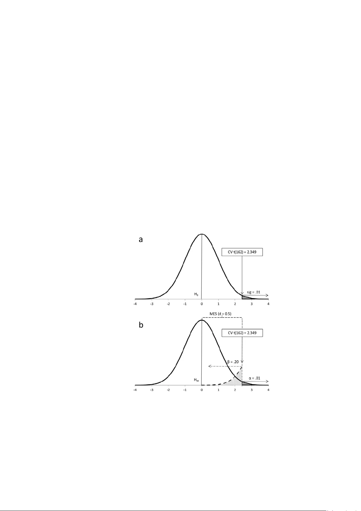
STATISTICAL SENSITIVE NESS - page 1 S tatistic al Sensitiveness for Science Jose D. Pe rezgonz alez Massey University , New Zeala nd Author’s note: Jose D. Perezgonzalez, Business School, Massey Unive rsity. Correspondence concerning this article should be addressed to Dr. Jose D. Perezgon zalez , Masse y University , Social Sciences T8.18, Manawatu Ca mpus, P.O. Box 11- 222, Palmerston North 4442, New Zealand. Phone: +6463505326, E- mail: j.d.perezgonzalez@massey.ac.nz STATISTICAL SENSITIVE NESS - page 2 Abstr act Research o ft en necessitat es of samples, yet obtaining large enough samples is not always possible. When it is, the researcher may use one of two methods for deciding upon the required s ample s ize: rul es -of-thumb, quick yet uncertain, and estimations for power, mathema tically pre cise yet with the potentia l to overestima te or und eresti mat e sample s izes when effect si zes ar e unknown. Misestimated sample sizes have nega tive repercussions in the form of i ncreas ed cos ts , abandoned projects or abandoned publication of non- sig nificant results . Here I desc ribe a procedur e for estim ating s ample s izes adequate fo r the testing approach which is most common in the behavioural , social , and bi omedical sci ences , that of Fisher’s te sts of significance . The pro cedure fo cus es on a desired minimum effect size for the research at han d and finds the minimum sample size re quired for capturin g such eff ect si ze as a statistica lly signific ant result. I n a similar fashion than power anal yses, sensitiveness analyses can also be extended to finding the minimum effect f or a given sample size a priori as well as to calculating sensitive ness a poste riori. The ar ticle provides a full tutorial for carr ying out a sensitiveness analysis, as well as empirical support via simulation . Keywor ds: sam ple si ze, s ensiti veness, power, Fisher, Ne yman - Pearson STATISTICAL SENSITIVE NESS - page 3 Intr oducti on Imag ine for a moment that y ou want to test the effect of a novel treatme nt on a dependent variable of interest. You intend to carry out an experiment with two independent groups using a test of sig nificance . How bi g ought your sample to be? In order to determine the appropriate sample size, y ou ma y consider wha t is typic al in your discipline, perhaps even cost or opportunity ( a procedure which is still quite common, as seen in re cent art icl es pu blis hed in Behaviour Research Methods , such as Caspar et al., 2015, Roncero & Almeida, 2015, and Widmer et a l. , 2015). Let’s say you opt for a sample of 30 participants. Reassured by tradition or good budgeting, you br ace your self for the best and hope for a s tatistic ally significant r esult. You may, however, feel that t his is not a very scientific way of setting a sample size and wish for a m ore rel iable pro ced ure . Sample size e stimation fo r power offers that reliable procedure fo r sett ing sam ple sizes, and t here now exist several desktop and online programs for effortle ss estimation . You thus download and run G*Power ( see also Faul, Erdfelder, Lang, & Buchner, 2007) and pretty much you get stuck: You can certain l y decide th e approp riate t est, w hether to use a one- tailed or a two - tailed test, a nd what informati on to enter fo r alp ha, allo cati on rati o , and , even, power; however, you have absolutely no idea about which effect size to use—how could you possibly know given that this is a novel treatment! It does not really ma tter how hard you think about it and how reasonable your arguments may be, at the end you are left t o just one resource: D ecide on an eff ect and s ee wh at sample si ze the program returns ; if t oo large, yo u m a y fiddle with the para meters until y ou reach a sati sfact or y comprom ise (something recommended by, for example, Cohen, 1988, and Lenth, 2001). I n hindsight, you probably still feel that this is ne ither more scientific nor mo re reliable th an the rules -of-thumb used earli er, yet it typically comma nds lar ger sam ples. In both cases get y our estimate righ t , and you are on y our way to a successful publication. Get it wro ng and use more participants than needed, and you would have brought about unnecessary harm (e.g., in the form of higher costs, anim als unneces sari ly sacri ficed , or excess patien ts unn ecess aril y harmed ). Even worse, get it reall y wrong by using less participants than needed, and the harm done spills to the whole sample as th e research p roj ect is fil ed awa y because results may not be publishable, unless you manage to motivate yourself to write up your “negati ve” resul ts as w ell as man age to get your paper i nt o one of the few journals that publish nonsignificant results. Is there a way out of this conundrum? Yes, there is ; t herefor e the goal s of this article: T o describ e the b ases of an alt ernativ e proced ure for estimating sample size s when we l ack enough knowledge about population effect sizes as for using power estimation, to support such procedure with e mpirical results from a serie s of simulations, and, finally, to provide a tutorial on h ow to reliably estimate sample sizes using such alternative procedure . As introduced above, a ccurat e estim ation of the r equ ired sam ple si ze for a res earch project ma y mean the d ifferen ce b etween a sig nificant test result and one confined to the file drawer, especially in the behavioural (Ioannidis, Munafò, Fusar-Poli, Nosek, & David, 2014), social ( Franco, Malhotra, & Simonovits, 2014), and b iomedi cal scien ces ( P apageorgiou, Papadopoulos, & Athanasiou, 2014). Two common approaches to sample estimation are rules -of-thumb and estimations for power. STATISTICAL SENSITIVE NESS - page 4 Rules -of-thumb represent quick heuristics for setting sample sizes. They m a y b e borne ou t of statistical principles (e .g. a sample size of 30 is about the min imum needed for rendering normal sampling distributions of means independently of whether the sample itself is normal ; A ron , Coups, & Aron, 2013; also Crawley, 2014). Or they may be linked to particu lar test s (e. g. , to χ 2 ; Van Voorhis & Morgan, 2007 ), to p articu lar procedures (e. g., to a factor anal ysis; Tab achni ck & Fi d ell , 2001), or to particula r goa ls (e. g. , to c osts; Van Belle, 2008). O ften enough , they are simply handed down as such rules- of -thumb (e.g., Cross Validated, 2014, “Rules of Thumb for Minimum Sample Size”, or Tools4Dev, 2014, “How to Choos e a Sampl e Siz e”). T hese ru les are indep end ent of an y particular r ese arch cont ex t and , thus, represent an i mprec ise appro ach t o setti ng sam ple si zes. Sample size e stimations fo r power were popularized by Co hen (1988) with his book Statistical Power Analysis for the Behavioral Sciences , which provided a one -stop shop for also cal culati ng the pow er of tests a posteriori and the si ze of effe cts — t he book is nowada ys supplanted by more convenient tools like propr ietary comput er so ftwar e , such as G*Power and SPSS SamplePo wer , and onl ine calcu lato rs , such as those provided on Daniel S opper.com. Unlike rules-of-thumb, power- based est imati ons ar e tai lored to particular research proj ects . Indeed, p ower an alysis provid es such good value to behavioural, social and bio medical research th at even grantees may ask fo r power anal yse s to be included with grant applications (e.g., National Institutes of Health, 2015; Voelker, 2014; Yale Institution for Social and Policy Studies, 2015 ). P ower , however, is circumscribe d to Ne yman and Pearso n’s app roach to d ata testin g (1933) and, thus, is mostly rel evant wh en res earch ers wo rk with competing precise hypotheses, know the eff ect si ze in t he popu latio n, assu me a rep eated s amp ling fr amew ork, and ar e concerned with controlling Type I and Type II error s in the long run (Perezgonzalez, 2015a ). Actuall y , N e ym a n - Pearson’s approach offers suc h good a priori control of the researc h environment that it is ide al for de signing simulations (e .g., Jo , 2002; Rast & H ofer, 2014; Siemer & Joormann, 2003; Simonsohn, Nelson, & Simmons, 2014; Stanley & Spence, 2014), even when sometimes such simulations ma y b e used for testing uns uitable research scenarios (e. g., Per ezgon zal ez, 2015b, c ). As it happens, mo st research i n the behaviou ral , soci al and bio m edical s cien ces does not work with repe ated s a mpling from the same population —often enough, it does not even define the effect size of intere st for differentia ting between h ypothes es nor control Type II errors a pri ori . Thus, it cannot be said to follow Neyman- Pearson’s approach. Instead, mo st of it defau lts to Fisher’s appr oach (e.g., 1960): T esti ng r esearch d ata a gainst a sin gle null hypothesis and ascert aining the ad hoc probabilit y of the research results against su ch hypothesis 1 . When using Fisher’s tests of significance, power anal yses are philosophica lly meaningl ess . S uch anal yses may als o for ce resea rchers to guess pop ulati on effe ct si zes an d may turn costly either because of an overestimation of the sa mple siz e so ca lculat ed —when the eff ect siz e is un derest imat ed —or because of underpowered research— when th e effe ct size is overe stimated . Furthermore , estimating effect siz es when no knowledge about the population exists, whether based on armchair thinking, guesses, hopes or wishful thinking, is also for eign to a cons cien tious research er a nd ethicall y questionable , whic h partly explains why power estimations have not yet managed to supplant rules-of-thumb in current research 1 Fishe r’s and Neyman - Pearson’s approaches are t ypi cally mixe d up into the philo sophicall y incohere nt null hypot hesis significanc e testing (NH ST) procedu re (Gigerenz er, 2004; Perezgonz alez, 2015 a). In t his article I will avoid re ferences to NHST, re ferring to the sounder approaches of Fisher and of Neym an - Pearson, instead. STATISTICAL SENSITIVE NESS - page 5 sampling (e.g., Button et al., 2013; Maxwell, Lau, & Howard, 2015; Va dill o, Konstantinidis, & Shanks, 2015). Indeed , ignoring power does not necess aril y affect si gnificanc e, as a tes t can re turn a significa nt result even if its pow er is low . What I d iscuss in this artic le is that s ensit iveness, not power, is the appropriate construct to attend to i n the case o f Fish er’s app ro ach: By incr easin g the siz e of the ex perimen t [ei ther b y enlargemen t o r repet itio n], we ca n render it more sensitive , meaning b y this that it will allow of the dete ction . . . of a quantitatively smaller departure from the null hypothesis . . . W e may say that the value of the experiment is increased whenever it permits the null hypothesis to be more readily disproved. (Fisher, 1960 pp. 21-22) Unfortunately , Fisher did not provide a method for controlling sensitiveness, th ereb y the purpose of this tutoria l . The rela tio nshi p bet ween p ower an d sensitivene ss Neyman, in particular, found Fisher’s dismissal of power troubling: It is now appropriate for me to mention a problem which obviously belongs to the categ ory of experimenta l tactics, but is miss ing in F isher's writings . . . The problem is that of the power of the tests contemplated for the treatment of the given experiment. The consideration of power is occasiona lly implic it in Fisher' s writings, but I w ould have liked to see it treated explicitly . (1967, p. 1459) Despite Neyman’s perception of the si milari ty bet ween pow er and s ensi tivenes s, Fisher’s d ismissal of power is understandable given that sensitiveness i s rooted in the different philosophi cal position and research goal of tests of sig nificance . As said earlie r , p ower is circ umscribed to Ney man -Pearson’s approach to data testin g (1933) and, thus, is most relevant when r esear ch h as the fol lowi ng param eters : A known effect size in the population which differentiates betwe en two statistic al hypotheses ( this effect size is provided by the alternative hypothesis); a Type I error probability (this is the probability of wrongly rejecting the main hypothesis under test in the long-run, under repeated sampling from the same population); and a Type II error probability (this is the probability of wrongly rejecting the alternative hypothesis in the long-run, under repeated sampling from the same population). The purpose of testing data is, primarily, to decide which h ypothes is ex plai ns the res earch d ata bet ter — a goal whi ch Fi sher co nsid ered more appropriate for industrial qualit y c ontrol than for c ontemporary research endeavours (Fisher, 1955). Fisher’s te sts of signi ficanc e , on the other hand, are tools for learnin g from the d ata at hand, ad hoc, without any f requentist assumption of repe ated samp lin g from the sam e population. It works despite not knowing the population effect size, not knowing the paramete rs of an al ternative h ypothesis, and not been interested in long-run errors linked to such hypothesis. Furthermore, the only purpose of testing data get s redu ce d to rej ect ing an otherwise uninformative null hypothesis (Perezgonzalez, 2015a). Despit e their d ifferen ces , N e ym a n - Pearso n’s procedure and Fisher’s procedure are intimately related , inasmuch Ney man- Pears on’s n ecessi tates of Fisher’s to test th e data. In a STATISTICAL SENSITIVE NESS - page 6 nutshell, a Neyman- Pearson’s test is a transduction of a n acceptance philosoph y onto a te st of signific anc e. Figu r e 1 r enders Fisher ’s an d Ne yman - Pearso n’s approach es to d ata test in g. Fi gu re 1A represen ts Fis her’s ap pro ach : a on e - tailed te st i n a t distributi on with 162 degree s of freedom. The distribution concerns a null h ypothesis ( H 0 ) with a conve ntional a re a of signifi cance at the 1% le vel. The level of significance ( sig ) represents a cu t -off point in such distribution, thus being also ass ociated to a pa rticu lar cri tical v alue ( CV ), even if this value is largely ignored when inte rpreting resu lts becaus e it is redundant with the more informative level of signifi canc e. N e ym a n - Pea rson ’s app roach (Figu re 1 B ) is t ypicall y represent ed by the distributions of both a main hy pothesis ( H M ) centered on ‘zero ’ and an alt ernat ive h ypot hesis cen tered on a different v a lue. The difference in location between these distributions (a.k.a., their degree of overlapping and nonoverlapping, Cohen, 1988) represents the effect size in the population (e.g., Cohen’s d = 0.5). The test, however, is carried out on the main hypothesis only, which is what Figure 1B represents (the reader may project the distribution of the alternative hypothesis by continuing the dashed lines off towards the right : T he dist ance b etween the mean s of the h ypothese s is the effect size ). The test represent ed in Fi gure 1B assumes a 1 % Type I error ( α ) and a 20 % Type II erro r ( β ). Figure 1 . Fisher ’s (a) and Ne yman - Pe arson’s (b) approach es t o data testing ( t -test for independent samples). STATISTICAL SENSITIVE NESS - page 7 As Figure 1 shows, both approaches are techni call y alike, more so when they coincide in using th e same test a nd distribut ion. I ndeed, Ne yman-Pearson’s alpha level doubles as the level of significance f or the test and c uts the distribution at the same cr itical value ( CV = 2.349) 2 . The onl y differen ce is that Ne yman - Pearso n’s appr oach al so inco rpo rates rel evant in formation provided by the alternative hypothesis: that is, the probability of making a T ype II error in the long run ( β ) and the population effect size. Before continuing our argument, however, a small detour is needed to explain what the eff ect siz e is, as this paramete r is cri tical for t he abovem entio ned ar gumen t. Let’s start with Fisher’s tests of significance. A te st of sign ificance is carrie d out in order to determine whether a phenomenon exists in the population or not. The hypothesis under test is that the phenomenon does not exist (e.g., H 0 = 0). However, the h ypothe sis is te sted against a particular frequency d istribution, e ffective l y allow ing other values than ‘zero’ to enter the test ( i.e., the assumption is that members of a population randomly show differing effects even when, in the aggregate, the phenomenon is not present in such population). Differ ent res ults within this frequency distribution will h ave different probabilities of occurrin g , extreme r esults being rarer and, thus , having smaller probabilities . T he level of sign ificance (e.g., sig ≈ .01 ) serv es as a convenient cut-off for making our mind in this respect, by comparing the observed probability of our research data ( p ) against the level of sign ificance. A larger p - valu e informs nothing, while the sma ller the p - value (e.g., p = .00 1) the m ore con fident we can b e that the research data do not fit t he null hypothesis well. The distribution shown in Figu re 1A rep resen ts a t distribution with 162 de grees- of - freedom: I t repres ents the density of frequencies around the mean value of ‘zero’ and al so provides the theoretical location of all possible resul ts ( t - values becom e lar ger th e furth er awa y from ‘zero ’) and t hei r associ ated p robabi lit y ( p - values b ecome s mall er the f urthe r awa y from ‘zero’). In a nutshell, each t - value has a p - val ue and ei ther can be u sed i nstead of the other (the p - value bei ng m ore convenient). Now, although Fisher did not work with effects sizes, it is possible to derive them from a tes t (e.g., Cohen, 1988, provided the appropriate formulas) . This means t hat an y t - value in our distribution can also b e ass ociated w it h a parti cular ef fect s ize i n the population—“To this point,” said Cohen (1988, p 11) “the ES [can be] considered quite abstract l y as a param eter w hich can t ake on var ying valu es (incl udin g zero i n the cas e of t he null cas e).” It also m eans that t he level o f si gnifica nce is a cut - off in the distributi on of t ’s (and, by extension, of associated p ’s and effect s izes ) in order to determine which shall be taken as ev iden ce a gainst H 0 and which shall not. It also imp lies that t ’s and p ’s can be us ed for estimating the true but unknown effect size in the population, especiall y when combined into a meta -analysis (Rosenthal, 1984; Braver, Thoemmes, & Rosenthal, 2014). A similar log ic is applic able to Ney man -Pearson’s tests (Figure 1B), with the particu larity that the se tests actu ally consider two overlapping distributions ( H M and H A ), separat ed b y a known effect s ize. This m eans that each possible location under H M will also appear und er H A (albeit with a different t - value and p -value), and that each effe ct si ze under H M is actu al l y a n eff ect s iz e under the now explicit H A ( bec ause the exp ected eff ect unde r H M = 0 ). N e ym an - Pea rson’s procedure is nonethele ss simplified by only testing the main 2 Neyma n - Pearson ’s alpha a nd Fisher’ s level of signi ficance ar e often confu sed and in distinctively called after each other (e.g., H ubbard , 2004). In th is article, I will d istinctl y differ entiate bet ween them to av oid confus ion (as recommend ed in Perez gonz alez, 2014). STATISTICAL SENSITIVE NESS - page 8 hypothesis using Fisher’s tests of si gnifican ce. Th erefore, the cut - o ff repr esen ted b y alp ha ( α = .01) not only determines which t ’s (and p ’s ) fall under H M and which fall under H A , it effecti vel y partiti ons th e effects exp ected und er the al ternat ive h ypoth esis i n to those important ones which will be accepted under H A and those unimportant ones which will be assumed under H M . (In Figure 1B, the information about the population effect size provided b y H A is thus repres ent ed b y MES, th e unimportant portion of the effect size param eter th at falls under H M .) In finishing our detour and returning to our argument, we can thus compare Figures 1A and 1B and readily ascertain that, apart from the nuances of β and MES incorporated b y N e ym a n -Pearson’s tests, the two approaches are techni call y alike . I ndeed, it is precisel y this overall technic al similarity that a llows resolving the problem of sensitiveness. Firstly, both Fisher and Neyman-Pearson end up carrying out a ( Fisher’s ) t est of signifi cance on a statistical hypothe sis centered on ‘zero’ (Fisher’s null hypothesis— H 0 —and N e ym a n -Pearson’s main hypothesis— H M —, respectively). As shown in Figure 1, for the case when both approaches coincide in using the same test and sampl e siz e, the th eoretical distribution for both tests is the s ame. Secondly , the lev el of si gni ficance ( sig ) and the probabilit y of Ty pe I error ( α ) are technic ally similar fo r any individua l test: Ne ym a n -Pearson’s alpha simply dou bles as Fisher’s l evel of si gnifica nce . As shown in Figure 1, t he sig / α level al so re sult s i n the sam e critical value ( CV ) and rejection region for both approaches when using the same distribution . Thirdly, as only the main hypothesis ( H M ) is tested under Neyman- Pearso n’s approach, it makes sense to represent just the proportional effect size, or minimum effect size ( MES ), that falls under H M . As shown in Figure 1B, ME S shares boundarie s with α , β , and CV , and has the f ollowing inter pretation: I t repres ents a region o f eff ects si zes un der the alterna tive hypothe sis which will be assu med to pertain to the main hypo thesis every time th e latter i s accep ted . Indeed, b ecaus e MES coincides with CV , we can s ee that it is MES , not the population effect s ize , which is used for the test. However, MES does not have an inhe rent meaning under Neyman-Pearson’s approach : In our example, it is eith er ES = d = 0 ( H M ) or ES = d = 0.5 ( H A ) which exp lains the research resul ts bet ter, not an y particu lar MES . Furthermore, altering α, β, N or the test (e.g., b y using a two- tail ed test) will alter CV a nd, consequentl y, MES , yet the population effe ct siz e remains the same. Thus, MES underlies N e ym a n - Pearson ’s tests yet does n ot n eed to be d eriv ed mat hemati call y because t he popul ation e ffect siz e is a mor e informative and convenient statistic . (T he in terest ed re ader may calcul ate it as shown later . In the case o f Fi gure 1B , the population effect siz e of Cohen’s d = 0.5 renders a n MES of d = 0.37.) As discussed by Cohen (1988), effect s iz es are properties of the populations of referenc e, not of stat isti cal t ests. Therefo re, des pite t he lack o f an ex pli cit alt ernativ e hypothesis, effect s izes are also co herent const ruc t s under Fisher’s approach. A minimum effect s ize can, thus, be d rawn i n a Fish er ’s t est dis tribution, sharing boundaries with sig and CV . Unlike Ney man -Pearson’s MES , however, Fisher’s MES is not a mathemat ical boundary between the distributions of two known hypotheses. Instead, it is an MES which the researcher decides upon as relevant to her research, independently of the actual distribution of the unknown alternative hypothesis. This MES does not depend on previous knowledge nor STATISTICAL SENSITIVE NESS - page 9 requires thinking about a population of reference: It may as well be decided upon ad hoc and it certainly accommodates wishful thinking as easil y as more considered reasoning. This is so because what is decided upon is the minimum effect size that would justify the cost of the research and its future implementation. (This idea is similar to L enth’s, 2001, lower bound on the effect size, for which he even proposed a procedure to help determine it, albeit in the context of power estimation.) In a nutsh ell, t he resear cher is not si mply thinking about obtaining a ny statistically significant result — a measu re of direction onl y—but about obtaining a statistica ll y sig nificant result for a de sired MES . Sai d other wise, th e research er is not simply aiming to diffe rentiate betwe en vague notewor th y results and those s he may ignore, but to decide how much is notewor thy — he r desi red min imum effect siz e and larg er effects —and to ensure that she has a la rge enough sam ple to capture s uch e ffects as statistically significant result s. Therefore, knowing the CV that co rrespon ds to t he des ired si gnifi cance l ev el allows for MES to be d erived m ath ematical l y — via the corresponding formulas for post hoc estimation , see Supplemental Table 1 — which , in our case, is equal to Cohen’s d = 0.37. (Notice that post hoc estimation of population effect sizes makes sense under Fisher’s, as t he approach works with the assumption that nothing is known about such effect sizes. This is unlike Neyman-Pearson’s approach, which starts with known effect sizes and, consequently, post h oc calcul ations of t he same a re me aningless .) Fourthly, and f inally , the problem of β cannot be resolved as it depends on an alternative hypothesis that Fisher’s approach does not consider. However, this problem can be circum vent ed with a proced ure t hat est imates sam ple si ze based on jus t sig and M ES . This procedur e esti m ates sensitiveness, defined as the mini mum sample size required for returning a sign ificant test res ult for a given (min imum) effect size. Simula tio n s using sensitive ness, power , and ru les - of - thumb In wishing to place the proce dure for estima ting sensiti veness at the end o f th e article, where it will be much easier to locate la ter on , I put the proverbial “cart b efo re the horse” and present t he results of sev eral simulations contr asting sa mple size estimation s for sensitiveness, for power, and when us in g a rul e -of-thumb. T raditiona l simulation s ba sed on repeated sampling from the same population are suitable f or Neyman - Pearson’s appro ach —in which population effect sizes are known—but not so for Fisher ’s —in which population effect sizes are not known. Ther ef ore, I designed a more suitable simulation program, based on generating multiple populations with relativ ely uncertai n param eters from which to e xtract the sample s. T he overall simulation program was run ‘manu all y’ and comprised e ight simulations (c alled ‘studies’), 43 inde pendent populations per study (thus, yielding 344 independent populations overall ) , three conditions per population (sensitiveness, power, and rule- of -thumb), and one independent sample per condition ( thus, yielding 129 samples per stud y a n d 1,032 samples in total— see Supplemental Material 3 for further information). Each research condition compri sed a t -test for independent groups using two groups of equal size: the rule-of-thumb condition used a total sample size of 30 (i.e., n = 15 pe r group), the power condition used a total sample size of 102 (i.e., n = 51 per group), and the sensitiveness condition used a total sample size of 48 (i.e., n = 24 per group). The power condition represent ed the sample size recommended for capturing Cohen ’s d = 0.5 with 80% STATISTICAL SENSITIVE NESS - page 10 power, and the sensitiveness condition represented the samp le siz e recomm ended for capturing Cohen’s d = 0.5 as a statistically significant minimum e ffect size ( MES ). The data of interest for analysis were the frequencies, or counts, o f effect s izes great er than Cohen’s d = 0.495 (to allow for rounding) which turned out to also be statistically signific ant ( sig ≤ .05). The inter est was for t he eff ect si ze to take prec eden ce over m ere statistical s ignifica nce, the reas onin g bei ng that a resear cher wh o does not know the eff ect size in the population but uses power analyses for deter mining sample size, most proba bly decides o n an eff ect si ze as t he min imum size he wishes to find— this effectivel y meant that both sign ificant yet s maller effe ct sizes an d nons ig nificant lar ger effect siz es were i gnor ed. For the analysis of frequencies, the target ef fect s ize was a medium eff ect ( Cohen’s w = .3). This MES meant t o be of enou gh size that a r easonabl e res earcher wo uld be s atisf ied that , compared to th e sm aller sam ple si ze recom mend ed b y the sensi tivenes s condition, whatever costs associ ated with t he larger s ample recomm ended b y the p ower condition (slightly ov er twice as la rge) would be justified by the bene fits it ma y bring (i.e., 30% or more tes ts capt ured) . S uch MES recom mend ed a s ample s ize of 4 3 per grou p for pai r comparisons ( χ 2 ) which i s t he sampl e siz e used pe r condition in each of the eight studies. F requenc y anal ys e s ( χ 2 for goodness-of- fit) we re thus carri ed out b etween pairs of conditions using the number of effect sizes greater than d = 0.495 that turned up as statistic al l y significant. Collate d results for the overall simulati on are pres en ted in Table 1 (and for each of the eight studies in Supp lement al Tabl e 4 ). Table 1 Significant tests which captured MES d > 0.495 (Frequen cies, P ercenta ges , Effect Sizes , and Test s of Significance) Condition Σf % Test w χ 2 p PWR 158 36.8 Pwr -Sns .03 0.26 .61 SNS 149 34.7 Sns- Thmb .10 2.69 .10 THMB 122 28.4 Thmb - Pwr .13 4.63 .03 Note . Σf = accumulated frequencies for significant tes ts capturing d > 0.495; PWR = power - based s ampling , SNS = se nsit ive nes s - ba se d sampling , T HMB = r ule - of - t hu mb - base d sampling . The simulation results show that , wh ile a lar ger sa mpl e tends t o also be more cap able of capturing the desi red effect siz es as statistically sig nificant, the difference betw een power - based sampling and sen siti veness -based sampli ng was rather unimportant ( w = .03, range [.03, .24], χ 2 = .26, p = .61). Surprisingly enough, although t he N = 30 - rul e -of-thumb-based sampling perfo rmed worse than sensiti veness -based sampling ( w = .10, range [.03, .33], χ 2 = 2.69, p = .10) a nd STATISTICAL SENSITIVE NESS - page 11 power- based sam plin g ( w = .13, range [.06, .26], χ 2 = 4.63, p = .03), the diffe rence in performan ce w as definitively s maller than the target MES set for the simulation. However , given that rules-of-thumb sampling recommendations are independent of research context, this ty pe of sampling may prove less relia ble than th e other two and I shall not disc uss it further . As for the sampling procedures of interes t , it is reasonable to conclude that power- based sam pli ng is not sensibl y bet ter than sens itiv eness -based sampling whe n used as intended in this artic le, yet it commands a larger sample siz e and, thus, is costlier . The resu lts of this simulatio n support the use of s ensit iveness anal y sis r ather t han powe r anal ysis when research desi gns are t ypi cal of th e form er. What now follows is a ba sic tutorial f or carrying o ut sens itiv eness anal y se s. Stati stical sensi tiveness an alysis (a tutorial ) Sample size es timation fo r sensitiveness In order to estima te sensitiveness, I devised the following two - step p rocess , to be iterate d until the requi red sampl e siz e for sens itiv eness is found: • The first step is to calculate the c ritical value o f a test that allows for rejecting a research resul t at a c ertai n level of signi fican ce. A s the l evel of s igni ficance remai ns fixed, t he onl y paramet er to manipulate is the sa mple size . Th is step can be conveniently performed with online calculators (e.g. DanielSoper.com) or by consulting appropriate tables. • The second step i s to c alculat e the e ffect s ize as sociat ed with above critical val ue b y using the appropriate formulas (Supplemental T able 1 ). This step can be conveniently performe d wit h online calculators (e.g. UCCS.edu) or it can be eas il y auto matiz ed using Excel. For exam ple, l et’s ass ume w e are int erest ed in esti mating th e minimum sample s ize capable o f captu ring an intergroup diffe rence eq ual to Coh en’s d = 0.37 (i.e., a small- to - medium effect s ize ) with a one- tailed t - test at the 1 % level of si gnifican ce . W e can open DanielS oper’s t value cal culat or (http://www.danielsoper.com/statcalc3/calc.aspx? id=10), enter a p robabi lit y level o f .01 , then ent er an y initial value as de grees o f freed om (let ’s sa y, 100). This will return the corresponding t value of 2.36. We then proceed to calculat e the associat ed effect size by using the corresponding formula— see Supplement al Table 1 —, which ret u rns a Cohen’s d = 0. 47. This d is lar ger than tar get MES , su ggesting that we need a larger sam ple in order t o cap ture the s mal ler tar get. Let’s ent er df = 2 00 and repeat above steps, which yields d = 0. 33, smaller than target M ES . With some fine - tuning, we will soon converge on df = 162, thus estimating N = 164 ( df = 162 + 2) as the minimu m sample size needed for capturing MES = d = 0. 37 as a statistically significant result (whi ch is what Fi gure 1A represen ts ). Table 2 provides a bre akdown of the sample sizes required for sensitiveness and power fo r Cohen ’s conv en tional effect siz es and for s everal stati stical tests (see also Supplemental Table 2). As shown, the required sample sizes for sensitiveness are markedly smaller than those required for power. T he reason for thes e diff erences i s t hat po wer tar gets STATISTICAL SENSITIVE NESS - page 12 an effect size in the population— ye t obscuring the fact th at it tests a minimum e ffect size in the sample — while sensitive ness targe ts a minimum effect size in the sample with out hoping to know the real effect size in the population. Table 2 Sample Sizes Required for Capturing Co hen’s Small, Medium and Large Effects test ES small medium large sns pwr sns pwr sns pwr t r 272 614 32 64 12 21 t d 275 620 48 102 21 42 χ²(1) w (1df) 384 785 43 88 16 32 χ²(2) w (2df) 594 964 67 108 24 39 χ²(3) w (3df) 774 1091 87 122 32 44 χ²(4) w (4df) 947 1194 106 133 38 48 χ²(5) w (5df) 1091 1283 124 143 45 52 F(1,dfd) f (2g) 389 788 66 128 29 52 F(2,dfd) f (3g) 605 969 102 159 44 66 F(3,dfd) f (4g) 789 1096 133 180 57 76 F(4,dfd) f (5g) 957 1200 161 200 68 80 F(5,dfd) f (6g) 1116 1290 188 216 80 90 Note. Sns (s ensiti vene ss ) = N needed for rej ecting Fi sher’s H 0 for sig = 5%. Pwr (p o we r ) = N needed for rejecting Neyman - Pearso n’s H M fo r α = 5%, β = 20%. t po int biserial r , t fo r indep end ent gr oups ; χ ² for goodne ss - of - fit, F oneway ANOVA . All tests are one - tailed. STATISTICAL SENSITIVE NESS - page 13 A priori sensit iveness analyses W hen a rese arch er is li mit ed to gi ven sample size s, a priori s ensiti veness an al yses provide information about the expecte d minimum ef fect size s for signifi can ce, so t hat the research er ma y ascert ain wh ether his res ear ch goal s are a chievabl e or n ot . • The first step i s to cal cul ate the cri tic al valu e of a test t hat corres ponds to t he desi red level of significance and sample siz e. This step can be conve nientl y performed with online calculators (e.g. DanielSoper.com). • The second step i s to c alculat e the e ffect s ize as sociat ed with above critical val ue b y using the appropriate formulas (Supplemental Table 1). Let ’s sa y we are interested in t esting mean differences between independent groups using a conventional level of significance ( sig = .05 ), a one- tai led test , and a sampl e siz e of N = 30. We ca n easil y find out the corre sponding cri tical value in a t distribution — t (28) = 1.70, p = .05—, then derive the minimum ef fect size tha t such sample size would be ab le to capture under th e circu mstan ces —Cohen’s d = 0.64. We are then in a good position to quer y whe ther our research, intervention or programme is capabl e of deli verin g at l east su ch medium- to - large effect siz e or, otherwise, whether we would be better of f incr easin g our sample size in order to c aptu re a sm aller effect s ize. (Incide ntally, this is the MES that the N = 30 rule- of - thumb was able to capture in the simulation.) Post - hoc sen sitiveness analyse s Post- hoc anal yses c an als o be perfo rmed for s ensiti veness . The fo rmul a is th e following: Positive values indicate over-sensitiveness and negative values indicate under- sensitiveness, both as a percent age of t he rati o bet ween a ctual and mini mum s ample s ize. As it happens with power, over- sensiti veness d ecr eases t he sti pulat ed MES , som ething which may fool a resear cher in to accepti ng a sm aller ME S simpl y because the test turned out statistically significant. Still, it is le ss of a concern than under-sensitiveness, which can be used for concluding nothing about a test res ult pr ecisel y becaus e it lacks enough sensitiveness for capturin g the ex pecte d minimum effect size. For exam ple, t he simulation describe d earlier was set up with enough sensitiveness ( N = 43 per condition and study ) to capt ure a med iu m - siz ed differen ce in fre quencies betw een pairs of conditions (Cohen’s w = .3). T herefor e, w e can ex pect t he N = 30 rule-of-thumb to be under- sensitiv e, some thing which it turned out to be, as it recommend ed a sampl e siz e 37.5% smaller than that required for sensiti veness. On the other hand, power-based sampling STATISTICAL SENSITIVE NESS - page 14 can be ex pected to be ov er -sensitive, which also turned out to be, as it recom mended a sampl e size 112.5% larger than that needed for s ens iti veness. Discussi on and c onclusi ons By now, t he read er has probabl y put the data presented in Table 2 to test u si ng G*Power and found that the sample size required for sensitiveness equals about 50% power (e. g. , N = 48 for a t test and medium- s ized d equals 52% power, and N = 43 for a χ 2 test with one degree of freedom and medium- siz ed w equals 50% power). Does this mean that the sensitivene ss analysis propo sed in this artic le ultimately fail s the res earch comm unit y by encouraging underpowered research? The answer to this riddle is ‘No’ , for several r easons now discussed. Firstly , as illustrated in Figure 1, sensitiv eness and powe r are related as they both share location with the cr itical valu e of the test . Ind eed, our r eader can deri ve t he effect siz e of the c ritical t used for a power- set test (e.g., for a medium- si zed d and 80% power) and realize th at it does not result in th e ‘ expect ed’ d = 0.5 but d = 0.37 (the MES ). This is so because Coh en’s post hoc formulas (see S upplemental Table 1 ) attempt to estimate unkn own population effect sizes — that is, the mid dle of the unknown alternativ e distribution —which tend to comprise about 50% power. Thus, the lower ‘power’ of sensitiveness is due to such formulation goal rather than to an inherent lack of power. In an y case, if th e read er goes down the table and onto more complex tests (i.e., those with more groups to take into account), he will find that as the number of groups increases so does the power. That is, the power equivalent to a sensitive medium- siz ed w with t hree degr ees - of freed om — χ 2 (3) — is 64%, while the power equivalent to a sensitive medium- sized f with six groups— F (5,dfd)— is 74%. Again, sensitiveness does not alway s imply low power. Secondly, although sens itiveness and power are related, the y are not nec essaril y the same. Inde ed , we could define power in terms of sensitiveness—80% power implies that the research sample i s l ar ge enough for a t est to be sensitive to 80% of effect sizes, i.e. those above MES —but not vice versa— a test may be sensitive and turn out sig nificant despite lacking po wer (e.g., Button et al., 2013; Maxwell, Lau, & Howard, 2015; Vadillo, Konstantinidis, & Shanks, 2015). Thirdly, power analysis assumes a known effect size, provided by the alternative hypothesis. Thus, a ny tim e such eff ect si ze is either known or can be reasonably set with some accu rac y, power i s th e best sampling strategy to use, precis el y becaus e it all ows for good control of the research context. Sensitiveness, on the other hand, is most appropriate when the researcher does not know the effect size in the population or when h e is after a particu lar minimum eff ect size . This seems to be the case wit h mos t current resea rch, whi ch tend to be pilot studies, pioneer research or overly based on Fisher’s approach (including most research done under the banner of null hypothesis significa nce testin g). This is to say , if research is oriented towards achievin g a desired minimum eff ect size , including in the vag ue form of a statistical result beyond a threshold of significance which may be used as evidenc e against a si ngl e nul l hypothesis, then sensitiveness is the most appropriate tool to use for sample e stimation. Last l y , a larg er sample will alway s trump a small er one. If a resear cher can afford a sample size in the thousands, she may as well discard both power and sensitiveness as a matter o f concer n ( anot her i ssue, o f cour se, is t he p ractical s igni fican ce of th e result s thereb y STATISTICAL SENSITIVE NESS - page 15 obtained). However, i f th e research er wi shes to tai lor th e sampl e size t o eit her a known eff ect size in the population or a d esired min imum effect size in the sa mple, then pow er analy sis and sens itiv eness anal ysis, resp ectivel y, will be th e appropriate strategies to use. In summary, I see sens iti veness as an impo rtant ad vance in t he math emat ical estimation of sample sizes a nd fitter - for -purpose than power analyses when using Fisher’s tests of significance. Thus, researchers following Fisher’s approach will benefit from estimating sample size f or sensitiveness in stead of for pow er. Furthermo re, wh at I present here is m erel y a st atistical technolog y. T he philosophical differen ces b etween Ne yman -Pearson’s and Fisher’s approaches are important and need to be considered for understanding the construct of effect size in the context of sensitiveness— namel y as the e ffect s ize ex pected i n the population of samples similar to the research sample (Fisher, 1955). Because philosophical considerations are often ign o red in r esearch work (Hager, 2013), I decided not to emphasise them in this artic le. STATISTICAL SENSITIVE NESS - page 16 Refer ences Aron, A., Coups, E. J., & Aron, E. (2013). Statistics for psychology (6th. ed.). Boston, MA : Pearson . Bluman, A. G. (2014). Elementary statistics. A step by step approach (9th ed.). New York, NY: McGraw - Hill. Braver, S. L., Thoemmes, F. J., & Rosenthal, R. (2014). Continuously cumulat ing meta - analysis and replicability. Perspect ives on Psych olo gical Science , 9 (3), 333-342. doi: 10.1177/1745691614529796 Button, K. S. , I oannidis , J . P. A., Mokrysz, C., Nosek, B. A., Flint, J., Robinson, E. S. J., & Munafò, M. R. (2013). Power f ailu re: wh y small sa mple size under mines the reliabi lit y of neuros cien ce. Nat u re Review s Neur osci ence, 14, 365-376. doi:10.1038/nrn3475 Caspar, E. A., Beir (de), A., Magalhaes De Saldanha Da Gama, P. A., Yernaux, F., Cleeremans, A., & Vanderborght, B. (2015). New f r ontiers in the rubber hand experiment: when a robotic hand becomes one’s own. Behaviour Research Methods, 47(3), , 744-755. doi: 1 0.3758/s13428-014-0498-3 Cohen, J. (1988). Statistic al power analysis for the behavioral sciences (2nd ed.). New York, NY: Ps yc hology Press. Cooksey, R. W. (2014). Illustrating statistical procedures. Finding meaning in quantitative data (2nd ed.). Prahran, Australia: Tilde. Crawley, M. J. (2014). Statistics: an introduction using R (2nd ed.). Chichester, UK: John Wiley & Sons. Cross Validat ed (2014 ). Rul es of Thumb for Minimum Sample Size for Multiple Regre ssion. StackExchange.com . Retrieved from http://stats.stackexchange.com/questions/10079/rules-of-thumb- for - minimum - samp le - size - for - multiple - reg ression Devore, J., Farnum, N., & Doi, J. (2014). Applied statistic s for enginee rs and scientists (3rd ed.). Stamford: Cengage Learning. Faul, F., Erdfelder, E., Lang, A. G., & Buchner, A. (2007). G*Power 3: A flexible statistical power analysis program for the social, behavioral, and biomedi cal scien ces. Behaviour Research Methods, 39 (2), 175-191. Field, A., Miles, J., & Field, Z. (2014). Discove ring statistics using R (1st ed. reprint.). London, UK: SAGE. Fish er , R. A. (1955). Statistical methods a nd scientific induc tion. Journal of the Royal Statistics Society, Series B (Methodological), 17, 69-78. Retrieved from http://www.jstor.org/stable/2983785 Fish er , R. A. (1960). The design of experiments (7th ed. ). Edinburgh, UK: Oliver & B o yd . Franco , A., Malhotr a, N. , & Simonovits, G. (2014). Publication bia s in the socia l sciences: unlocking the file drawer. Science , 345 (6203) , 1502-1505. doi: 10.1126/science.1255484 Gigerenzer, G. (2004). Mindless statistics. The Journal of Socio-Economics, 33 , 587-606. doi:10.1016/j.socec.2004.09.033 Ha ger , W. (2013). The statistical theories of Fisher and of Ne y man and Pearson: a methodological perspective. Theory & Psychol ogy, 23 (2) , 251-270. doi: 10.1177/0959354312465483 Harris, M., & Taylor, G. (2014). Me dical statistics mad e easy (3rd ed.). Banbury, UK: Scion. STATISTICAL SENSITIVE NESS - page 17 Healey, J. F. (2015). Statistics. A to ol for social rese arch (10th ed.). Stamford, CT: Cengage Learning. Hinton, P. R. (2014). Statistics e xplained (3r d ed.). Hove, UK: Routled ge. Hubbard, R. (2004). Alphabet soup. Blurring the distinctions between p’s and α’s in psycholo gical resear ch. Theory & Psychology, 14 (3), 295-327. doi:10.1177/0959354304043638 Ioannidis, J. P. A., Munafò, M. R., Fusar-Poli, P., Nosek, B. A., David , S. P. (2014). Publication and other reporting biases in cognitive scie nces: det ection , prev alence, and prevention. Trends in Cogn itive Sciences, 1 8 (5), 235-241. doi:10.1016/j.tics.2014.02.010 Jackson, S. L. (2014). Statistics plain and simple (3rd ed.). Wadsworth, CA: Cengage Lea rn in g. Jo, B. (2002). Statistical power in randomized intervention studies with noncompliance. Psychological Methods , 7 (2), 178-193. doi: 10.1037/1082-989X.7.2.178 Lenth, R. V. (2001). Some practical guidelines for effective sample size determination. The American Statistician, 55 (3), 187-193. doi: 10.1198/000313001317098149 MacGillivray, H., Utts, J. M., & Heckard, R. F. (2014). Mind on statistic s (2nd ed.). Austral ia: C engage Learni ng. Maxwell, S. E., Lau, M. Y., & Howard, G. S. (2015). Is psychology suffering from a replica tion crisis? What doe s “ failur e to repl icat e” reall y mean? America n Psychologist, 70 (6), 487-498. doi:10.1037/a0039400 Moore, D. S., & Notz, W. I. (2014). Statistics. Concepts and controversies (8th ed.). New York, NY: W. H. Freeman. Moore, D. S., Notz, W. I., & Fligner, M. A. (2015). The basic pra ctice of statistic s (7th ed.). New York, NY: W . H. Freem an. National I nstitutes of Hea lth (2015, Septem ber 2 5 ) . Collabora tive Activities to Pro mote Metabol omics Resear ch. Retriev ed from htt p://grants.nih.gov/grants/guide/pa- files/PA -15-030.html Neyman, J. (1967). R. A. Fisher (1890-1962): an appreciation. Science, 156 (3781), pp. 1456- 1460. N e ym a n , J ., & Pearso n , E. S. (1933). On the prob lem of the most eff icient tests of sta tistical hypotheses. Philosophical Transactions of the Royal Society of London. Series A, Containing Papers of a Mathematical or Physical Character, 231 , 289-337. Retrieved from http://www.jstor.org/stable/91247 Papageorgiou, S. N., Papadopoulos, M. A., Athan asiou , A.E. (2014) . Assessing sma ll study effects and pub licati on bias in orthodontic meta- anal yses: a meta - epidemiological study. Clin ical Oral Investigations, 18 (4 ), 1031-1044. doi: 10.1007/s00784-014- 1196-3 Perezgonzalez, J. D. (2014). A reconceptualization of significance testing. Theor y & Psychology , 24(6), 852-859. doi:10.1177/0959354314546157 Perezgonzalez, J. D. (2015a). Fisher, Neyman-Pearson or NHST? A tutorial for teaching data testing . Frontiers in Psychology, 6 (223), 1-11. doi:10.3389/fps yg.2015.00223 Perezgonzalez, J. D. (2015b). Confidence intervals and tests are two si des o f the sam e research question. Frontiers in Psychology, 6 (34), 1 -2. doi:10.3389/fpsyg.2015.00034 Perezgonzalez, J. D. (2015c ). Commenta ry: Continuously cumulating me ta - anal ysis and replica bility. Frontiers in Psychology, 6 (565), 1-2. doi:10.3389/fpsyg.2015.00565 Rast, P., & Hofer, S. M. (2014). Longitudinal design considerations to optimize power to detect var iances and co vari ances am on g rates of chang e: Sim ulati on resu lts b ased on actual lo ngitudinal studie s. Psychological Methods, 19 (1 ), 133-154. doi: 10.1037/a0034524 STATISTICAL SENSITIVE NESS - page 18 Roncero, C., & Almeida (de), R. G. (2015). Semantic prop erties, ap tness, familiarity, conventionality, and interpretive diver sit y scores for 84 metaphors and similes. Behaviour Research Methods, 47 (3) , 800-812. doi: 10.3758/s13428-014-0502-y Rosenthal, R. (1984). Meta -analytic procedures for social research . Beverly Hills, CA: Sage. Siemer, M., & Joormann, J. (2003). Power and measures of effect size in analysis of variance with fixed versus random nested factors. Psycholo g ical Methods, 8 (4), 497-517. doi: 10.1037/1082-989X.8.4.497 Simonsohn, U., Nelson, L. D., & Simmons, J. P. (2014). P- curve and eff ect si ze. C orrecti ng for publication bias using only significant results. Perspecti ves on Ps ychol og ical Science, 9 (6), 666-681. doi: 10.1177/1745691614553988 Stanley, D. J., & Spence. J. R. (2014). Expectations f or replication s. Are yours re alistic? Perspect ives on P sycho lo gical S cience, 9 (3), 305-318. doi: 10.1177/1745691614528518 Tabachnick, B . G., & Fidell, L . S. (2001) . Usi ng multivariate statist ics (4th ed.). Boston, MA: Allyn & Bacon. Tools4Dev (2014). How to Choose a Sample Size (for the Statistically Challenged). Tools4Dev.org . Retrieved from http://www.tools4dev.org/resources/how- to -choose-a- sample - size Utts, J. M., & Heckard, R. F. (2015). Mind on statistics (5th ed.). Stamford, CT: Cengage Lea rn in g. Vadillo, M. A., Konstantinidis, E., & Shanks, D. R. (2015). Underpowered samples, false negatives, and unconscious learning. Psychono mic B ullet in & Review , 1-16. doi:10.3758/s13423-015-0892-6 Van Belle, G. (2008). Statistical ru les of thumb (2 nd ed.). Hoboken, N.J.: Wiley. VanVoorhis, C. R. W., Morgan, B. L. (2007). Understanding power and rules of thumb for determin ing sample sizes . Tutorials in Quantitative Methods for Psychology, 3 (2), 43 ‐ 50. Voelker, R. (2014). Stay the course. Monitor on Psychology, 45 , 60. Retriev ed from http://www.apa.org/monitor/2014/07-08/stay-course.aspx Widmer, C. L., Wolfe, C. R., Reyna, V. F., Cedillos-Whynott, E. M., Brust-Renck, P. G., & Weil, A. M. (2015). Tutorial dialogues and gist explanations of genetic breast cancer risk. Behaviour Research Methods, 47 (3) , 632-648. doi: 10.3758/s13428-015-0592-1 Yale I nstitution for Social a nd Policy Studie s (2015, Sep tember 2 5). ISPS Grant Applica tion . Retriev ed from http://isps.yale.edu/c ontent/isps - gran t -application#.VG6DFGec4nE STATISTICAL SENSITIVE NESS - page 19 Supplement al material 1 Supplemental Table 1 Effect Size Formulas and Cohen’s Conve ntional Effect Size Values r ; small = 0.10; medium = 0.30; large = 0.50 d ; small = 0.20; medium = 0.50; large = 0.80 w ; small = 0.10; medium = 0.30; large = 0.50 f ; small = 0.10; medium = 0.25; large = 0.40 STATISTICAL SENSITIVE NESS - page 20 Supplemental mat erial 2 Supplemental Table 2 Target and Actual Effect Sizes, Sample Sizes and Critical Test Values target ES N CV (sig < .05) actual ES small r = .1 272 t(270) = 1.6514 r = .1000 medium r = .3 32 t(30) = 1.7225 r = .3000 large r = .5 12 t(10) = 1.8257 r = .5000 small d = 0.2 275 t(273) = 1.6505 d = 0.1998 medium d = 0.5 48 t(46 ) = 1.6787 d = 0.4950 large d = 0.8 21 t(19) = 1.7291 d = 0.7934 small w = ϕ = .1 384 χ²(1) = 3.8415 ϕ = .1000 medium w = ϕ = .3 43 χ²(1) = 3.8415 ϕ = .2989 large w = ϕ = .5 16 χ²(1) = 3.8415 ϕ = .4900 small w = V(2) = .071 594 χ²(2) = 5. 9915 V(2) = .0710 medium w = V(2) = .212 67 χ²(2) = 5.9915 V(2) = .2115 large w = V(2) = .354 24 χ²(2) = 5.9915 V(2) = .3533 small w = V(3) = .058 774 χ²(3) = 7.8147 V(3) = .0580 medium w = V(3) = .173 87 χ²(3) = 7.8147 V(3) = .1730 large w = V (3) = .289 32 χ²(3) = 7.8147 V(3) = .2853 small w = V(4) = .050 947 χ²(4) = 9.4877 V(4) = .0500 medium w = V(4) = .150 106 χ²(4) = 9.4877 V(4) = .1496 large w = V(4) = .250 38 χ²(4) = 9.4877 V(4) = .2498 small w = V(5) = .045 1091 χ²(5) = 11.0705 V(5) = .0450 medium w = V(5) = .134 124 χ²(5) = 11.0705 V(5) = .1336 large w = V(5) = .224 45 χ²(5) = 11.0705 V(5) = .2218 small f = 0.10 389 F(1,387) = 3.8656 f = 0.0999 medium f = 0.25 66 F(1,64) = 3.9909 f = 0.2497 large f = 0.40 29 F(1,27) = 4.2100 f = 0.3949 small f = 0.10 605 F(2,602) = 3.0107 f = 0.1000 medium f = 0.25 102 F(2,99) = 3.0882 f = 0.2498 large f = 0.40 44 F(2,41) = 3.2257 f = 0.3967 STATISTICAL SENSITIVE NESS - page 21 target ES N CV (sig < .05) actual ES small f = 0.10 789 F(3 ,785) = 2.6162 f = 0.1000 medium f = 0.25 133 F(3,129) = 2.6748 f = 0.2494 large f = 0.40 57 F(3,53) = 2.7791 f = 0.3966 small f = 0.10 957 F(4,952) = 2.3813 f = 0.1000 medium f = 0.25 161 F(4,156) = 2.4296 f = 0.2496 large f = 0.40 68 F(4,63) = 2.5177 f = 0.3998 small f = 0.10 1116 F(5,1110) = 2.2222 f = 0.1000 medium f = 0.25 188 F(5,182) = 2.2638 f = 0.2494 large f = 0.40 80 F(5,74) = 2.3383 f = 0.3975 STATISTICAL SENSITIVE NESS - page 22 Suppl em ental mater ia l 3 Simulatio n environme nt The ove rall simulation st r ategy aime d to recr eate a t yp i c a l res earch con tex t with the following character istics: • Single res ear ch proje cts r ather t han repeated samp ling from the same population. The overall resear ch thus comprised a total of 1,032 tests carried out on 1,032 independent sampl es ext racted from 344 independent populations of differing size. The populations and sam ples were simulated as follows: o In order to prevent repeated sampling from the same population, f our macro - populations were gen erated for the s imul ation. Thes e macro -populations run from larg e to small ( N = 20,000, N = 10,000, N = 4 ,000, and N = 2 ,000), compri sed two equ al - sized independe nt groups, and were randoml y ge nerated in Ex cel (with group parameters N ~1 0,1 and N ~1 0.5,1) as for representing a medium- effect s ize di fferen ce betw een gro ups (C ohen ’s d = 0.5). ( We ma y think about macro-populations as representing psy cholo gical disorders with different prevalence internationally (e.g., major depression, rather prevalent, and schizophrenia , rather rare). Becau s e t h e y are i nternational macro - populations, they are inaccessible (research is done on local populations, instead) ; and becaus e the y are ina ccessib le, th e re al effect siz es of disorders, although assumed fixed, are unknown. This is w h y simulated macro - populations with known parameters are not suitable for testing Fisher’s approach as such, thus the next step.) o In o r der to i ncreas e local un certaint y re gardin g the param eter s of the m acro - populations, independent research populations were ra ndoml y extracte d fro m above mac ro -populations using SPSS. The extraction c riteria were twofold: siz e ( N = 2 ,000 and N = 1 , 000 wer e ex tracted fro m m acro -population 20,000; N = 2 ,000 and N = 500 from macro -population 10, 000; N = 1 ,000 and N = 200 from macro -population 4,000; and N = 500 and N = 200 were ext racted f rom macro -population 2,000) and independence (e ach resear ch population was created anew for each roun d, totalling 43 independent populations per study and 344 populations over all) . ( We may think about populations as repres enting p reval ence of psychological disorders at regio nal lev els. Becau se it cannot be reaso nabl y exp ected for all disorders to be proportionall y distributed around the world, but, perhaps, that personality disorders are more prevalent in one count ry while schizophrenia is more prevalent in another, the populations w ere not ne ces saril y extracted in a manner proportional to the size of the macro -populations. Furt hermo re, it can not be ex pected that res ear chers from differ ent parts of a r egi on will acc ess the entire population but, instead, that they will access local subsets of such population, even when the intention is to ge neralize to the whole population. I n order to mimic this, each population was extracted independently, further i ncreasin g the un cert aint y about the parameters for each local population. Notice that at this point, t he exact ef fect s ize for ea ch l ocal population as well a s the ex act mean s an d standard deviations per group are unknown a priori, which is what the exercise STATISTICAL SENSITIVE NESS - page 23 attempted to achieve — i. e., although it is reasonable to think that they are not far from the initial known pa rameters, it is imp ossible to say with certainty. Indeed, Supplemental Table 3 provides summary statistics for populations at “regional” levels, starting to show random deviations from the initial paramete rs ; consequentl y, greater uncertainty is expected for each individual “local” population, from which the samp les were t aken .) o To better mimic the sing le - study ad hoc ap p roach of a t ypical r esea rch proj ect, research samples wer e then random l y selected fro m each population per s t u d y condition ( k = 3) using SPSS, totalling 1,032 samples overall . Supplemental T able 3 Descriptiv e Statistics for Eight Simulated Populati ons Statistic I II III IV V VI VII VIII N 1 5000 10000 2000 2000 1000 10000 5000 1000 Mean 1 10.00 9.99 10.01 9.97 10.03 10.00 10.00 10.03 SD 1 1.00 1.00 0.98 1.02 1.02 1.00 1.00 1.02 N 2 5000 10000 2000 2000 1000 10000 5000 1000 Mean 2 10.48 10.51 10.49 10.52 10.48 10.48 10.48 10.48 SD 2 1.01 0.99 1.01 1.01 1.02 0.99 1.01 1.02 d 0.48 0.53 0.48 0.55 0.45 0.49 0.48 0.45 Research N 2000 2000 1000 200 200 1000 500 500 PWR , % sig 72.1 86.0 79.1 90.7 69.8 76.7 86.0 74.4 SNS, % si g 55.8 48.8 37.2 53.5 44.2 58.1 53.5 37.2 THMB, % sig 23.3 37.2 37.2 44.2 30.2 44.2 41.9 32.6 Note . N = Macro - population size (per group), Research N = t otal size of each of 43 independent research populat ions ( eac h generated in o rder to draw a s ingle random sam ple per con dition ). % s i gn = per centage of significant tests irrespectiv e of effect size considerations , dou bling as an indi cator of pow e r . PWR = power - based s ampling ( n = 102), SNS = sensitiveness - based sa mp l ing ( n = 48 ), THMB = rule - of - thumb - based sam pling ( n = 30). • The simulatio n also tried to mimic resea rch contexts when, despite the r eal effect size in the population being unknown, a researcher nonetheless decides to use an effect size both for purposes of sampling estimation and of result interpretation. The mini mum effect siz e consid ered meani ngful, reas onabl e or de fendabl e was set, “coincidentally”, to be Cohen’s d = 0.5 , subject to the statistic al signif icance of a tes t. (The minimum e ffect size ough t to be th e same t han t he effect siz e desi gned fo r the simulation at ma cro -population levels in order to make a meaningful comparison between conditions without unnecessary extraneous complications.) Larger effect STATISTICAL SENSITIVE NESS - page 24 sizes which w ere also statistic ally signif icant were, or course, acceptable, thus counted, while smaller effect sizes were considered untenable and, thus, ignored irrespe ctively of their statistical signif icance. (T his procedure give s a great er rol e to practical si gnific ance than to statistical sig nificance; othe rwise, a larger sample will always be more powerful and, thus, return a significant result for smaller effects, even when the r esear cher h ad deci ded a priori that those effects were unimportant. That is, while a la rger sample a lwa ys trumps a smalle r one, statistica l significa nce typically trumps ef fect sizes, which is what the rese arch tri ed to av oid .) • The conditions under test were the three sampling strategies discussed in the main article: o Power -based sampling. C onventional parameters we re plug ged into G*Power : one- tailed t test (between groups), ES = 0.5, α = .05, power = .80, ratio allocation = 1, which recommended a total sample of n = 102 ( i.e., n = 51 per group). This condition thus represents a reasonable procedure followed b y a res earcher who does not know, and does not wish to double- gues s, th e real effect size in the population , yet is still inte rested in a particular minimum effect size. Because Cohen (1988) does not talk about MES , such res ear cher only has the resource of pluggi ng in the d esired effect siz e and of lat er ignor ing a significant r esult whose eff ect size is smaller th an desire d. o Sensi tiven ess -based sampling. The a priori procedure for sensitiveness was run also using conventional parameters: t test, sig = .05, and ES = 0.5. The minimum total samp le size re commended was n = 48 (i.e., n = 24 per group). This condition thus represents the sampling approach discussed in this document: c arrying o ut a significance te st but ensuring th at it is sensitive enough to capture the desired ( minimum) eff ect size. Because this desired MES is independent of the unknown population effect siz e, a resear che r may carry on without concerning herself with double-guessing the la ter. o Rule-of-thumb sampling. U sin g n = 30 , this condition repres ents th e use o f a rule -of-thumb independentl y of the particularities of the research project. In aiming for sound yet economic sampling, a researcher may opt for this rule-of- thumb, as it “promises” normal sampling distributions adequate for t - tests (e. g. , Crawle y, 2014). • Analyses focused on the frequency of significant t tests which cap tured th e specifi ed effect s ize o r large r . T he di fference i n count s b etween pairs of cond itio ns were tes ted using χ 2 for goodness - of - fit. T herefore, the effect s iz e took preceden ce over st atist ical signifi cance so that a t te st was not co unted if the eff ect size was smalle r than expect ed (i.e. , d < 0.495, for rounding purposes) or if the test was not significant. The target MES for χ 2 was a m edium effect s ize ( w = .30), which recommended a minimum sample si ze of N = 43 per c ondition and stud y. The overall simulation was broken down into eight studies, each study including 43 independent research populations of similar size and comprising 129 independent samples. The overall simulation amounted to 1,032 samples. Supplemental Table 3 collates the main descrip tive statistics f or the eight studies . Suppl emental Table 4 (as wel l as Tabl e 1) co llates th e main res ults of the simulation (frequ encies, p erc entages , χ 2 tests , and effect s izes ). As can b e observed, most paired STATISTICAL SENSITIVE NESS - page 25 comparisons turned out to be below the set threshold for a minimum eff ect of modera te size ( w = .30), and the only one which turned out statistically significant was just about moderate in size ( w = .33 ). The agg regated to tal fu rther i llus trates t hat th e diff erence b etween power and sensitiveness- based sampling is rather neg ligible ( w = .03) when a res earche r seeks a minimum effe ct size and no t merely statistical significa nce. Surprisingly enough, the N = 30 rule- of -thumb did not fare too bad either. Although it certainl y shows a small effect s ize ( w ≥ .10), it fared re lative l y well un der the crite rium used for the simulation in the first place. In any case, given the ra ndom selection of samples, we can be confident that no bias other than random variability was present in the simulation, and we m a y d eem t he effect si zes ob tained reliabl e desp ite th e lack of s tatis tical signi fican ce. Thus, we can conclude that the sampling strategies using power and sensitiveness were sensib ly more b enefi cial to the research than the N = 30 rule- of - thumb in the case of this simulation. Suppl emental Table 4 Simulation Resul ts (Freq uencies , Per centages , Te sts , and Eff ect Sizes) Statistic I II III IV V VI VII VIII All studies f PWR 17 18 21 28 16 19 23 16 158 f SNS 20 21 13 22 18 20 20 15 149 f THMB 10 16 16 18 13 18 17 14 122 % PWR 36.2 32.7 42.0 41.2 34.0 33.3 38.3 35.6 36.8 % SNS 42.6 38.2 26.0 32.4 38.3 35.1 33.3 33.3 34.7 % THMB 21.3 29.1 32.0 26.5 27.7 31.6 28.3 31.1 28.4 χ 2 PWR - SNS 0.24 0.23 1.88 0.72 0.12 0.03 0.21 0.03 0.26 w 0.08 0.08 0.24 0.12 0.06 0.03 0.07 0.03 0.03 χ 2 SNS - THMB 3.33 0.68 0.31 0.40 0.81 0.11 0.24 0.03 2.69 w 0.33 0.14 0.10 0.10 0.16 0.05 0.08 0.03 0.10 χ 2 THMB - PWR 1.82 0.12 0.68 2.17 0.58 0.87 0.34 0.72 4.63 w 0.26 0.06 0.14 0.22 0.14 0.15 0.09 0.15 0.13 Note . Statist ics for signif icant tes ts captu ring d > 0.49 5. Each study tested 43 in dependen t sam ples pe r conditi on (i.e., 12 9 sam ples per study , and 1,032 sam ples in tota l). f = fre quencies for sign ificant tests ca pturing d > 0.495; PWR = power - bas ed samplin g ( n = 102), S N S = se nsiti vene s s - based s ampling ( n = 48), THMB = rule - of - thumb - based sam pling ( n = 30). P - values intentio nally o mitted, a s they offer less valuab le infor mation than target minimum effect size ( w = .30).