Safe Probability

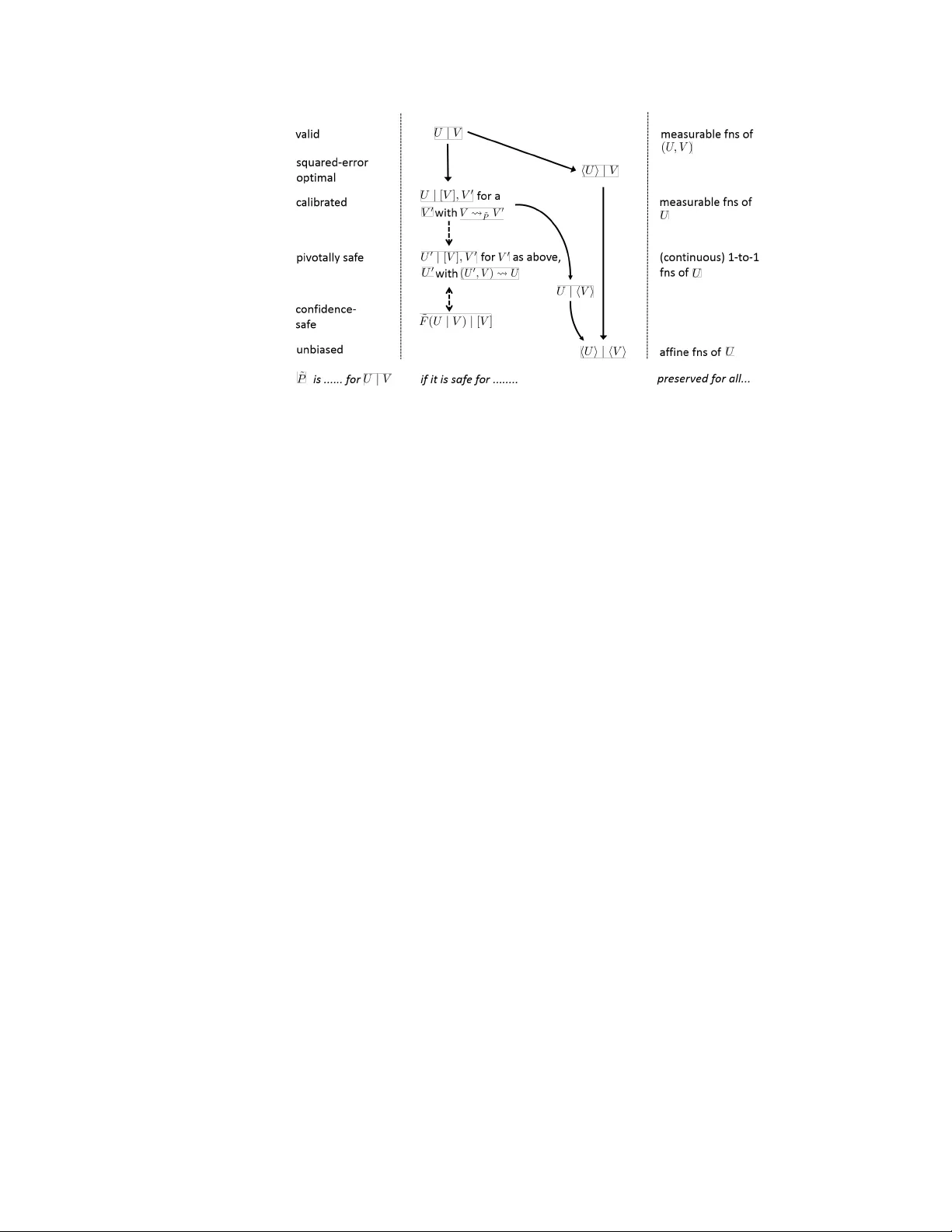
Safe Probabilit y P eter Gr ¨ un wald April 8, 2016 Abstract W e formalize the idea of probabilit y distributions that lead to reliable predictions ab out some, but not all asp ects of a domain. The resulting notion of ‘safet y’ provides a fresh persp ectiv e on foundational issues in statistics, providing a middle ground b etw een imprecise probabilit y and multiple-prior mo dels on the one hand and strictly Bay esian approac hes on the other. It also allows us to formalize ﬁducial distributions in terms of the set of random v ariables that they can safely predict, th us taking some of the sting out of the ﬁducial idea. By restricting probabilistic inference to safe uses, one also automatically a voids parado xes such as the Mon t y Hall problem. Safety comes in a v ariety of degrees, such as ‘v alidit y’ (the strongest notion), ‘calibration’, ‘conﬁdence safety’ and ‘un biasedness’ (almost the weak est notion). 1 In tro duction W e formalize the idea of probability distributions that lead to reliable predictions about some, but not all aspects of a domain. V ery broadly speaking, we call a distribution ˜ P safe for predicting random v ariable U given random v ariable V if predictions concerning U based on ˜ P ( U | V ) tend to b e as go o d as one would exp ect them to b e if ˜ P were an accurate description of one’s uncertaint y , even if ˜ P may not represent one’s actual b eliefs, let alone the truth. Our formalization of this notion of ‘safety’ has rep ercussions for the foundations of statistics, pro viding a join t p ersp ective on issues hitherto viewed as distinct: 1. All mo dels are wrong... 1 Some statistical models are evidently b oth entirely wrong y et very useful. F or example, in some highly successful applications of Bay esian statistics, suc h as latent Dirichlet allo cation for topic mo deling (Blei et al., 2003), one assumes that natural language text is i.i.d., whic h is ﬁne for the task at hand (topic mo deling) — yet no-one w ould wan t to use these mo dels for predicting the next w ord of a text given the past. Y et, one can use a Bay esian p osterior to make suc h predictions any w ay — Bay esian inference has no mechanism to distinguish b etw een ‘safe’ and ‘unsafe’ inferences. Safe probability allo ws us to imp ose such a distinction. 2. The Eternal Discussion 2 More generally , represen ting uncertaint y by a single distri- bution, as is standard in Ba y esian inference, implies a willingness to mak e deﬁnite predictions ab out random v ariables that, some claim, one really knows nothing ab out. Disagreemen t on 1 ...y et some are useful, as famously remarked by Box (1979). 2 When the single-vs. multiple-prior issue came up in a discussion on the de cision-the ory forum mailing list, the well-kno wn economist I. Gilboa referred to it as ‘the eternal discussion’. 1 this issue go es bac k at least to Keynes (1921) and Ramsey (1931), has led many economists to sympathize with multiple-prior mo dels (Gilb oa and Sc hmeidler, 1989) and some statisticians to embrace the related impr e cise pr ob ability (W alley, 1991, Augustin et al., 2014) in whic h so-called ‘Knightian’ uncertaint y is mo deled b y a set P ∗ of distributions. But imprecise probabilit y is not without problems of its own, an imp ortant one b eing dilation (Example 1 b elo w). Safe probability can b e understo o d as starting from a set P ∗ , but then mapping the set of distributions to a single distribution, where the mapping inv ok ed ma y dep end on the prediction task at hand — thus av oiding b oth dilation and ov erly precise predictions. The use of suc h mappings has b een adv o cated b efore, under the name pignistic tr ansformation (Smets, 1989, Hamp el, 2001), but a general theory for constructing and ev aluating them has b een lacking (see also Section 5). 3. Fisher’s Biggest Blunder 3 Fisher (1930) in tro duced ﬁducial infer enc e , a metho d to come up with a ‘p osterior’ ˜ P ( θ | X n ) on a mo del’s parameter space based on data X n , but without anything like a ‘prior’, in an approac h to statistics that was neither Bay esian nor frequen tist. The approach turned out problematic how ev er, and, despite progress on related structur al infer enc e (F raser, 1968, 1979) was largely abandoned. Recently , how ev er, ﬁducial distributions ha ve made a comeback (Hannig, 2009, T araldsen and Lindqvist, 2013, Martin and Liu, 2013, V eronese and Melilli, 2015), in some instances with a more modest, frequentist in terpretation as c onﬁdenc e distributions (Sc hw eder and Hjort, 2002, 2016). As noted b y Xie and Singh (2013), these ‘con tain a wealth of information for inference’, e.g. to determine v alid conﬁdence in terv als and un biased estimation of the median, but their interpretation remains diﬃcult, viz. the insistence b y Hamp el (2006), Xie and Singh (2013) and many others that, although ˜ P ( · | X n ) is deﬁned as a distribution on the parameter space, the parameter itself is not random. Safe probability oﬀers an alternativ e p ersp ective, where the insistence that ‘ θ is not random’ is replaced b y the w eaker (and p erhaps lib erating) statemen t that ‘w e can treat θ as random’ as long as we r estrict ourselves to safe infer enc es ab out it ’ — in Section 3.1 w e determine precisely what these safe inferences are and how they ﬁt into a general hierarch y: 4. The Hierarch y Pursuing the idea that some distributions are reliable for a smaller subset of random v ariables/prediction tasks than others, leads to a natural hier ar chy of safeties — a ﬁrst taste of which is in Figure 1 on page 5, with notations explained later. At the top are distributions that are fully reliable for whatev er task one has in mind; at the b ottom those that are reliable only for a single task in a weak, av erage sense. In b etw een there is a natural place for distributions that are c alibr ate d (Example 2 b elo w), that are c onﬁdenc e–safe (i.e. v alid conﬁdence distributions) and that are optimal for squar e d-err or pr e diction . 5. “The concept of a conditional probability with regard to an isolated hypoth- esis... 4 Up on ﬁrst hearing of the Mont y Hall (quiz master, three do ors) problem (vos Sa v an t, 1990, Gill, 2011), most p eople naively think that the probability of winning the car is the same whether one switches do ors or not. Most can even tually , after muc h arguing, b e 3 While Fisher is generally regarded as (one of ) the greatest statisticians of all time, ﬁducial inference is often considered to b e his ‘big blunder’ — see Hamp el (2006) and Efron (1996), who writes Mayb e Fisher’s biggest blunder wil l b e c ome a big hit in the 21st c entury! 4 ... whose probability equals 0 is inadmissible,” as remarked b y Kolmogorov (1933). As will b e seen, safe probabilit y suggests an ev en more radical statement related to the Mon ty Hall sanity chec k. 2 con vinced that this is wrong, but wouldn’t it b e nice to hav e a simple sanity chec k that im- me diately tells y ou that the naive answer must b e wrong, without even p ondering the ‘right’ w ay to approach the problem? Safe probability pro vides such a chec k: one can immediately tell that the naive answer is not safe , and thus cannot b e righ t. Such a c heck is applicable more generally , whenev er conditioning on ev en ts rather than on random v ariables (Example 4 and Section 4). 6. “Could Neyman, Jeﬀreys and Fisher hav e agreed on testing? 5 Ry abko and Monarev (2003) sho ws that sequences of 0s and 1s pro duced by standard random num b er generators can b e substan tially compressed by standard data compression algorithms such as rar or zip . While this is clear evidence that such sequences are not random, this metho d is neither a v alid Neyman-Pearson hypothesis test nor a v alid Ba yesian test (in the tradition of Jeﬀreys). The reason is that b oth these standard paradigms require the existence of an alternative statistic al mo del , and start out by the assumption that, if the null mo del (i.i.d. Bernoulli (1/2)) is incorrect, then the alternative must b e correct. How ev er, there is no clear sense in which zip could b e ‘correct’ — see Section 5. There is a third testing paradigm, due to Fisher, whic h does view testing as accum ulating evidence against h 0 , and not necessarily as conﬁrming some precisely speciﬁed h 1 . Y et Fisher’s paradigm is not without serious problems either — see Section 5. Berger et al. (1994) started a line of w ork culminating in Berger (2003), who presents tests that ha ve in terpretations in all three paradigms and that av oid some of the problems of their original implemen tations. Ho wev er, it is essen tially an ob jectiv e Ba yes approach and th us inevitably , strong evidence against h 0 implies a high p osterior probabilit y that h 1 is true. If one is really doing Fisherian testing, this is unw an ted. Using the idea of safety , w e can extend Berger’s paradigm by stipulating the inferences for whic h we think it is safe: roughly sp eaking, if w e are in a Fisherian set-up, then w e declare all inferences conditional on h 1 to be unsafe, and inferences conditional on h 0 to b e safe; if we really b elieve that h 1 ma y represen t the state of the world, w e can declare inferences conditional on h 1 to b e safe. But muc h more is p ossible using safe probability — a DM can decide, on a case by case basis, what inferences based on her tests would b e safe, and under what situations the test results itself are safe — for example, some tests remain safe under optional stopping, whereas others (ev en Bay esian ones!) do not. While we will rep ort on this application of safety (which comprises a long pap er in itself ) elsewhere, w e will brieﬂy return to it in the conclusion. 7. F urther Applications: Ob jective Ba yes, Epistemic Probabilit y Apart from the applications abov e, the results in this pap er suggest that safe probabilit y b e used to formalize the status of default priors in obje ctive Bayesian inferences, and to enable an alternative look at epistemic pr ob ability . But this remains a topic for future work, to which w e brieﬂy return at the end of the pap er. The Dream Imagine a w orld in whic h one would require an y statistical analysis — whether it b e testing, prediction, regression, density estimation or an ything else — to be accompanied b y a safety statement . Such a statement should list what inferences, the analysists think, can b e safely made based on the conclusion of the analysis, and in what formal ‘safety’ sense. Is the alternative h 1 really true even though h 0 is found to b e false? Is the suggested predictiv e 5 ...”, as asked b y Jim Berger (2003). 3 distribution v alid or merely calibrated? Is the p osterior really just go o d for making predictions via the predictiv e distribution, or is it conﬁdence-safe, or is it generally safe? Do es the inferred regression function only work well on cov ariates drawn randomly from the same distribution, or also under cov ariate shift? (an application of safety we did not address here but which we can easily incorporate). The present, initial form ulation of safe probabilit y is too complicated to hav e any realistic hop es for a practice lik e this to emerge, but I can’t help hoping that the ideas can b e simpliﬁed substan tially , and a safer practice of statistics might emerge. Starting with Gr ¨ un wald (1999), my own work — often in collab oration with J. Halpern — has regularly used the idea of ‘safety’, for example in the context of Maximum Entrop y inference (Gr ¨ un wald, 2000), and also dilation (Gr ¨ unw ald and Halp ern, 2004), calibration (Gr ¨ unw ald and Halp ern, 2011), and probabilit y puzzles like Mont y Hall (Gr ¨ un wald and Halp ern, 2003, Gr ¨ un wald, 2013). How ev er, the insights of earlier papers were v ery partial and scattered, and the presen t pap er presents for the ﬁrst time a general formalism, deﬁnitions and a hierarc hy . It is also the ﬁrst one to make a connection to conﬁdence distributions and pivots. 1.1 Informal Overview Belo w we explain the basic ideas using three recurring examples. W e assume that we are giv en a set of distributions P ∗ on some space of outcomes Z . Under a frequentist interpreta- tion, P ∗ is the set of distributions that w e regard as ‘p oten tially true’; under a sub jectivist in terpretation, it is the cr e dal set that describ es our uncertain ty or ‘b eliefs’; all developmen ts b elo w work under b oth interpretations. All probability distributions men tioned below are either an element of P ∗ , or they are a pr agmatic distribution ˜ P , which some decision-maker (DM) uses to predict the outcomes of some v ariable U given the v alue of some other v ariable V ,where b oth U and V are random quan tities deﬁned on Z . ˜ P is also used to estimate the quality of such predictions. ˜ P (whic h ma y b e, but is not alwa ys in P ∗ ) is ‘pragmatic’ b ecause we assume from the outset that some elemen t of P ∗ migh t actually lead to b etter predictions — we just do not kno w which one. Example 1 [Dilation] A DM has to make a prediction or decision ab out random v ariable U ∈ U = { 0 , 1 } given the v alue of V ∈ V = { 0 , 1 } . She kno ws that the marginal probability P ( U = 1) = 0 . 9; she susp ects that U ma y dep end on V , but has no idea whether U and V are p ositively or negatively correlated or how strong the correlation is. She may thus mo del her uncertaint y as the set P ∗ of al l distributions P on Z = U × V that satisfy P ( U = 1) = X v ∈V P ( U = 1 , V = v ) = 0 . 9 . (1) Giv en that V = 1, what should she predict for U ? A standard answer in imprecise probabilit y (W alley, 1991) is to p oin twise condition the set P ∗ , leading one to adopt the probabilities P ∗ ( U = 1 | V = 1) := { P ( U = 1 | V = 1) : P ∈ P ∗ } . But this set contains every distribution on U , including P ( U = 1 | V = 1) = 0 (the latter would obtain for the P ∈ P ∗ with P ( U = | 1 − V | ) = 1). It therefore seems that, after observing V = 1, the DM has lost rather than gained information. By symmetry , the same happ ens after observing V = 0, so whatever DM observes, she loses information — a phenomenon kno wn as dilation (Seidenfeld and W asserman, 1993). This is intuitiv ely disturbing, and it ma y p erhaps b e better to simply 4 Figure 1: A Hierarc hy of Relations for ˜ P . The concepts on the right corresp ond (broadly) to existing notions, whose name is giv en on the left (with the exception of U | h V i , for whic h no regular name seems to exist). A → B means that safety of ˜ P for A implies safet y for B — at least, under some conditions: for all solid arrows, this is pro ven under the assumption of V with countable range (see underneath Prop osition 1). F or the dashed arrows, this is prov en under additional conditions (see Theorem 2 and subsequent remark). On the right are sho wn transformations on U under whic h safety is preserved, e.g. if ˜ P is calibrated for U | V then it is also calibrated for U 0 | V for ev ery U 0 with U U 0 (see remark underneath Theorem 2). W eakening the conditions for the pro ofs and providing more detailed interrelations is a ma jor goal for future work, as well as inv estigating whether the hierarc hy has a natural place for c ausal notions, suc h as ˜ P ( U | do ( v )) as in Pearl’s (2009) do-calculus. ignor e V and predict using the distribution that acts as if U ⊥ V and has ˜ P ( U = 1 | V = v ) = P ( U = 1) for all v ∈ V , (2) i.e. ˜ P ( U = 1 | V = v ) = 0 . 9. While from a purely sub jective Bay esian standpoint information is never useless and this seems silly , it is certainly what humans often do in practice, and usually , they get aw a y with it (Dempster, 1968) — for concrete examples see Gr ¨ unw ald and Halp ern (2004). Here is where Safe Probability comes in — it tells us that ˜ P is safe to use, in the following simple sense : for any function g : U → R , we hav e: for all P ∈ P ∗ , all v ∈ V : E U ∼ P [ g ( U )] = E U ∼ ˜ P [ g ( U ) | V = v ] . (3) In particular, if w e hav e a loss function L : U × A → R mapping outcomes and actions to asso ciated losses, then, for any action a ∈ A , we can plug in g ( U ) := L ( U, a ) ab ov e and then w e ﬁnd that (assuming P ∗ con tains the truth): DM’s predictions are guaranteed to b e exactly as go o d, in exp ectation, as she would exp e ct them to b e if ˜ P wer e actual ly ‘true’ — even if ˜ P is not true at all. W e immediately add though that if w e had a loss function L 0 : U × V × A → R which would itself dep end on V (e.g. if V = 1 DM is oﬀered a diﬀerent b et on U than if V = 0) then the ˜ P based on ignoring V is not safe any more — (3) may not hold an y more, and the actual exp ectation may b e diﬀerent from DM’s. In terms of the formalism we develop b elo w 5 (Deﬁnition 1, 2 and 3), this will b e expressed as ‘ ˜ P is safe for predicting with loss function L but not loss function L 0 ’, or, in formal notation, ˜ P is safe for L ( · , a ) | [ V ] but not for L 0 ( · , a ) | [ V ]. The in tuitive meaning is that DM can safely use ˜ P to make predictions against L (her predictions will b e as go o d as she exp ects) but not against L 0 . These statements will b e immediate consequences of the more general statements ‘ ˜ P is safe for U | [ V ] but not safe for U | V ’. In some cases, we will not b e able to come up with a ˜ P satisfying (3), and we hav e to settle for a ˜ P that satisﬁes a weak er notion of safety , such as, for all P ∈ P ∗ , all functions g , E V ∼ P  E U ∼ ˜ P [ g ( U ) | V ]  = E U ∼ P [ g ( U )] , (4) whic h says that DM predicts as well on av erage as DM would exp ect to predict on av erage if ˜ P were true, even though ˜ P may not b e true. This will b e denoted as ‘ ˜ P is safe for U | h V i ’; and if (4) only holds for g the iden tity (which mak es no diﬀerence if |U | = 2, but in general it do es) we hav e the even weak er safety for h U i | h V i (Figure 1). In Section 2.2 w e th us obtain ﬁve basic notions of safety , v arying from weak safety , in an av erage sense, to very strong safety , safet y for U | V , which essen tially means that ˜ P ( U | V ) must b e the correct conditional distribution. In this example we used frequentist terminology , such as ‘correct’ and ‘true’, and we con tin ue to do so in this pap er. Still, a sub jective interpretation remains v alid in this and future examples as well: if the DM’s real b eliefs are given by the full set P ∗ , she can safely act as if her b elief is represented b y the singleton ˜ P as long as she also b elieves that her loss do es not dep end on V . Example 2 [Calibration] Consider the w eather forecaster on your lo cal television station. Ev ery night the forecaster makes a prediction about whether or not it will rain the next da y in the area where you live. She do es this b y asserting that the probabilit y of rain is p , where p ∈ { 0 , 0 . 1 , . . . , 0 . 9 , 1 } . Ho w should w e interpret these probabilities? The usual in terpretation is that, in the long run, on those days at which the weather forecaster predict probabilit y p , it will rain approximately 100 p % of the time. Th us, for example, among all da ys for which she predicted 0 . 1, the fraction of days with rain was close to 0 . 1. A w eather forecaster (DM) with this prop erty is said to b e c alibr ate d (Da wid, 1982, F oster and V ohra, 1998). Lik e safet y itself, calibration is a minimal requirement: for example, a w eather forecaster who predicts, each day of the year, that the probability of rain tomorrow is 50% will b e approximately calibrated in the Netherlands, but her predictions are not v ery useful — and it is easily seen that, when using a prop er scoring rule, optimal forecasts are calibrated, but calibrated forecasts can b e far from optimal. On the other hand, in practice w e often see calibrated w eather forecasters that predict w ell, but do not predict with an ything close to the ‘truth’ — their predictions dep end on high-dimensional cov ariates consisting of measuremen ts of air pressure, temp erature etc. at n umerous lo cations in the w orld, and it seems quite unlikely (and, for practical purp oses, unnecessary!) that, giv en an y sp eciﬁc v alues of these co v ariates, they issue the correct conditional distribution. While calibration is usually deﬁned relative to empirical data, a re-deﬁnition in terms of an underlying set of distributions P ∗ is straightforw ard (V ovk et al., 2005, Gr ¨ un wald and Halp ern, 2011), and in Section 2.3 we show that the probabilistic deﬁnition of calibration has a natural expression in terms of the safet y notions introduced ab ov e: ˜ P ( U | V ) is calibrated for U if it is safe for U | [ V ] , V 0 , for some V 0 with V V 0 (all notation to b e explained) — which implies that (3) is itself an instance of calibration. 6 Example 3 [Ba yesian, Fiducial and Conﬁdence Distributions] W e are given a para- metric probabilit y mo del M = { q θ | θ ∈ Θ } where Θ ⊆ R k for some k ≥ 1, each q θ deﬁnes a probabilit y density or mass function on data ( X 1 , . . . , X N ) = X N of sample size N , eac h outcome X i taking a v alue in some space X . The goal is to make inferences ab out θ , based on the data X N or some statistic S ( X N , N ) thereof. In the common case with ﬁxed N = n and inference based on the full data, S ( X N , N ) := X n , we can transfer this statistical sce- nario to our setup by deﬁning P ∗ as a set of distributions on Z = Θ × X n . R Vs U and V = S ( X n , n ) = X n are then deﬁned as, for each z = ( θ , x n ), U ( z ) := θ and V ( z ) := x n . DM emplo ys a set Π of prior distributions on Θ, where each π ∈ Π induces a joint distribution P π on Θ × X n with marginal on Θ determined by π and, given θ , density of x n giv en by q θ , so that if π has densit y p π , we get the join t density p π ( θ , x n ) = p π ( θ ) · q θ ( x n ). W e set P ∗ := { P π : π ∈ Π } to b e the set of all such joint distributions. In the sp ecial case in which DM really is a 100% sub jective Bay esian who b eliev es that a single prior π captures all un- certain ty , we ha ve that P ∗ = { P π } contains just a single join t parameter-data distribution, and w e are in the standard Ba yesian scenario. Then DM can set ˜ P ( θ | X n ) := P π ( θ | X n ), the standard p osterior, and an y type of inference ab out θ is safe relative to P ∗ . Here we fo cus on another sp ecial case, in which Π con tains exactly one density for eac h θ ∈ Θ, namely the degenerate distribution putting all its mass on θ . W e denote this distribution b y P θ and notice that then P ∗ = { P θ : θ ∈ Θ } , with P θ (Θ = θ ) = 1, and for an y measurable set A , P θ ( X n ∈ A ) determined b y density p θ , satisfying p θ ( x n ) = p θ ( x n | Θ = θ ) = q θ ( x n ) . Still, any c hoice of pragmatic distribution ˜ P ( U | V ) = ˜ P ( θ | X n ) can b e in terpreted as a distribution on U ≡ Θ given the data X n , analogous to a Bay esian p osterior. In Section 3 w e inv estigate how one can construct distributions ˜ P of this kind that are safe for inference ab out c onﬁdenc e intervals . for simplicity we restrict ourselv es to the 1-dimensional case, for whic h w e ﬁnd that the construction w e pro vide leads to ˜ P that are conﬁdence-safe, written in our notation as ‘safe for ˜ F ( U | V ) | [ V ]’, with ˜ F b eing the CDF (cumulativ e distribution function) of ˜ P ( U | V ). Conﬁdence safety is roughly the same as co verage Sweeting (2001): it means that the ‘true’ probability that θ is con tained in a particular t yp e of α -credible sets (sets with ‘p osterior’ probability α given the data V ), is equal to α . The ˜ P w e construct are essentially equiv alent to the c onﬁdenc e distributions of (Sch w eder and Hjort, 2002), that were designed with the explicit goal of having go o d conﬁdence prop- erties; they also often coincide with Fisher’s 1930 ﬁducial distributions, which in later work (Fisher, 1935) he started treating as ordinary probability distributions that could b e used without any restrictions. This cannot b e right (see e.g. (Hamp el, 2006, page 514)), but the question has alw ays remained how a probability calculus for ﬁducial distributions could b e deriv ed that incorp orates the right restrictions. Our work pro vides a step in this direction, in that we show ho w such ˜ P sn ugly ﬁt in to our general framework: conﬁdence safety is a strictly w eaker prop erty than calibration, and has again a natural represen tation in terms of the h U i | h V i notation mentioned abov e. Moreov er, it is a sp ecial case of pivotal safety whic h also has rep ercussions in quite diﬀerent contexts — see Example 4. The example illustrates tw o imp ortant p oin ts: 1. In some cases the literature suggests some metho d for constructing a pragmatic ˜ P . An example is the latent Dirichlet allo cation mo del (Blei et al., 2003) mentioned ab ov e, in 7 whic h data V are text corp ora, P ∗ , not explicitly given, is a complicated set of realistic distributions ov er V under which data are non-i.i.d., and the literature suggests to tak e ˜ P ( U | V ) as the Bay esian p osterior for a clev erly designed i.i.d. mo del. 2. In other cases, DM may wan t to construct a ˜ P herself. In Example 1, the safe ˜ P was obtained by replacing an (unknown) conditional distribution with a (known) marginal — a sp ecial case of what was called C -conditioning b y Gr ¨ un wald and Halp ern (2011). Marginal distributions and distributions that ignore asp ects of V play a more cen tral role in this construction pro cess: they also do in the conﬁdence construction mentioned ab o ve, where one sets ˜ P ( U | V ) equal to a distribution such that ˜ P ( U 0 | V ), where U 0 is some auxiliary random v ariable (a pivot ), b ecomes indep enden t of V . F or the original R V U though, in the dilation example, DM acts as if U and V are indep endent ev en though they may not b e; in the conﬁdence distribution example, DM acts in a ‘dual’ manner, namely as if U and V are dep endent, even though under P ∗ they are not — whic h is ﬁne, as long as her conclusions are safe . Example 4 [Ev en t-Based Conditioning and Pivotal Safet y via Mon ty Hall] More generally , we ma y look at safet y for pragmatic distributions ˜ P that condition on ev ents rather than random v ariables. T o illustrate, consider the Mont y Hall Problem (vos Sav ant, 1990, Gill, 2011): supp ose that you’re on a game show and given a c hoice of three do ors { 1 , 2 , 3 } Behind one is a car; b ehind the others are goats. Y ou pick do or 1. Before op ening do or 1, Mon ty Hall, the host op ens one of the other tw o do ors, say , do or 3 which has a goat. He then asks y ou if you still w ant to take what’s be hind do or 1, or to tak e what’s b ehind do or 2 instead. Should you switc h? Y ou may assume that initially , the car was equally lik ely to b e b ehind each of the do ors and that, after y ou go to do or 1, Mon ty will alwa ys op en a do or with a goat b ehind. Basically y ou observe either the even t { 1 , 3 } (if Mont y op ens do or 2) or { 1 , 2 } (if Mont y op ens 3). Y ou can then calculate y our optimal decision according to some distribution ˜ P ( { 1 } | E ), where E ∈ {{ 1 , 3 } , { 1 , 2 }} is the even t you observed. Naiv e conditioning suggests to tak e P ( { 1 } | { 1 , 2 } ) = P ( { 1 } | { 1 , 3 } ) = (1 / 3) / (2 / 3) = 1 / 2, and it tak es a long time to convince most p eople that this is wrong — but, if DM’s w ould adhere to safe probability , then no convincing and explanation w ould be needed: translation of the example in to our ‘safety’ setting immediately shows, without an y further thinking ab out the problem, that this choice of ˜ P is unsafe , under all notions of safety we consider! (Section 4). Another asp ect of the Mont y Hall problem is that, in most analyses that are usually view ed as ‘correct’, one implicitly assumes that the quiz master ﬂips a fair coin to decide whether to op en do or 2 or 3 if y ou choose do or 1 so that he has a choice. There ha ve b een heated discussions (e.g. on wikip edia talk pages) ab out whether this assumption is justiﬁed. In Example 11 w e show that the ˜ P whic h assumes a fair coin ﬂip by Mon ty is an instance of a pivotal ly safe pragmatic distribution. These hav e the prop erties that for many loss functions (including 0 / 1-loss as in Mon ty Hall), they lead one to making optimal decisions. Thus, while assuming a fair coin ﬂip may b e wrong, it is still harmless to base one’s decisions up on it. Ov erview of the P ap er In Section 2, we treat the case of countable space Z , deﬁning the basic notions of safet y in Section 2.2 (where we return to dilation), and showing how calibration can b e cleanly expressed using our notions in Section 2.3. In Section 3 w e extend the setting to general Z , which is needed to handle the case of conﬁdence safet y (Section 3.1), piv ots (Section 3.2) and squared error optimality , where we observ e contin uous-v alued random 8 v ariables. Section 4 brieﬂy discusses non-numerical observ ations as w ell as probability updates that cannot b e view ed as conditional distributions. W e end with a discussion of further p oten tial applications of safety as well as op en problems. Pro ofs and further technical details are delegated to the app endix. 2 Basic Deﬁnitions for Discrete Random V ariables F or simplicit y , we introduce our basic notions only considering countable Z , which allows us to sidestep measurabilit y issues altogether. Thus b elow, Z is countable; we treat the general case in Section 3. 2.1 Concepts and notations regarding distributions on Z W e deﬁne a random v ariable (abbreviated to R V) to b e an y function X : Z → R k for some k > 0. Thus R Vs can b e m ultidimensional (i.e. what is usually called ‘random vector’). By an ‘ Y -v alued R V’ or simply ‘generalized R V’ w e mean an y function mapping Z to an arbitrary set Y . F or tw o R Vs U = ( U 1 , . . . , U k 1 ) , V = ( V 1 , . . . , V k 2 ) where U j and V j are 1-dimensional random v ariables, we deﬁne ( U, V ) to b e the R V with comp onents ( U 1 , . . . , U k 1 , V 1 , . . . , V k 2 ). F or any generalized R Vs U and V on Z and function f we write U f V if for all z ∈ Z , V ( z ) = f ( U ( z )). W e write U V (“ U determines V ”, or equiv alently “ U is a c o arsening of V ”) if there is a function f such that U f V . W e write U ! V if U V and V U . F or tw o GR Vs U and V w e write U ≡ V if they deﬁne the same function on Z , and for a distribution P ∈ Z we write U = P V if P ( U = V ) = 1. W e write U f P V if P ( { z ∈ Z : V ( z ) = f ( U ( z )) } ) = 1, and U P V if there exists some f for which this holds. Clearly U V implies that for all distributions P on Z , U P V , but not vice v ersa. Let S : Z → S b e a function on Z . The r ange of S , denoted range ( S ), the supp ort of S under a distribution P , and the range of S given that another function T on Z tak es v alue t , are denoted as range ( S ) := { s ∈ S : s = S ( z ) for some z ∈ Z } ; supp P ( S ) := { s ∈ S : P ( S = s ) > 0 } , range ( S | T = t ) = { s ∈ S : s = S ( z ) for some z ∈ Z with t = T ( z ) } (5) where we note that supp P ( S ) ⊆ range ( S ), with equality if S has full supp ort. F or a distribution P on Z , and U -v alued R V U , w e write P ( U ) as short-hand to denote the distribution of U under P (i.e. P ( U ) is a probability measure). W e generally omit double brac kets, i.e. if we write P ( U, W ) for R Vs U and W , we really mean P ( R ) where R is the R V ( U, W ), An y generalized R V that maps all z ∈ Z to the same constan t is called trivial , in particular the R V 0 which maps all z ∈ Z to 0. F or an ev ent E ⊂ Z , we deﬁne the indic ator r andom variable 1 E to b e 1 if E holds and 0 otherwise. Conditional Distributions as Generalized R Vs F or given distribution on Z and gen- eralized R Vs V and W , w e denote, for all v ∈ supp P ( V ), P | V = v as the conditional distribution on Z given V = v , in the standard manner. W e further deﬁne ( P ∗ | W = w ) := { ( P | W = w ) : P ∈ P ∗ , w ∈ supp P ( W ) } to b e the set of distributions on Z that can b e arriv ed at from P by conditioning on W = w , for all w supp orted by some P ∈ Z . 9 W e further denote, for all v ∈ supp P ( V ), P ( U | V = v ) as the conditional distribution of U given V = v , deﬁned as the distribution on U given b y P ( U = u | V = v ) := P ( U = u, V = v ) /P ( V = v ) (whereas P | V = v is deﬁned as a distribution on Z , P ( U | V = v ) is a distribution on the more restricted space range ( U )). Supp ose DM is interested in predicting R V U giv en R V V and do es this using some conditional distribution P ( U | V = v ) (usually this P will b e the ‘pragmatic’ ˜ P , but the deﬁnition that follows holds generally). Adopting the standard conv en tion for conditional exp ectation, we call an y function from range ( V ) to the set of distributions on U that coincides with P ( U | V = v ) for all v ∈ supp P ( V ) a version of the conditional distribution P ( U | V ). If we make a statement of the form ‘ P ( U | V ) satisﬁes ...’, we really mean ‘ev ery v ersion of P ( U | V ) satisﬁes...’. W e thus treat P ( U | V ) as a E -v alued random v ariable where E = { P ( U | V = v ) : v ∈ range ( V ) } , where, for all z ∈ Z with P ( V = V ( z )) > 0, P ( U | V )( z ) := P ( U | V = V ( z )), and P ( U | V )( z ) set to an arbitrary v alue otherwise. Unique and W ell-Deﬁnedness Recall that DM starts with a set P ∗ of distributions on Z that she considers the right description of her uncertaint y . She will predict sume R V U giv en some generalized R V V using a pr agmatic distribution ˜ P . F or R V U : Z → R k and generalized R V V , we say that, for giv en distribution P 0 on Z , P 0 ( U | V ) is essential ly uniquely deﬁne d (relativ e to P ∗ ) if for all P ∈ P ∗ , supp P ( V ) ⊆ supp P 0 ( V ) (so that P -almost surely V takes v alue v with P 0 ( V = v ) > 0). W e use this deﬁnition b oth for P 0 ∈ P ∗ and for P 0 = ˜ P ; note that we alw ays evaluate whether P 0 is uniquely deﬁned under distributions in the ‘true’ P ∗ though. W e say that E P 0 [ U | V ] is well-deﬁned if, writing U = ( U 1 , . . . , U k ), and, U + j = max { U j , 0 } , U − j = max {− U j , 0 } , we ha ve, for j = 1 ..k , either E P 0 [ U + j | V ] < ∞ with P -probability 1, or E P 0 [ U − j | V ] < ∞ with P -probability 1. This is a very w eak requirement that ensures that calculating exp ectations never inv olv es the op eration ∞ − ∞ , making all exp ectations w ell-deﬁned. The Pragmatic Distribution ˜ P W e assume that DM makes her predictions based on a probabilit y distribution ˜ P on Z whic h we generally refer to as the pr agmatic distribution . In practice, DM will usually b e presented with a decision problem in whic h she has to predict some ﬁxed R V U based on some ﬁxed R V V , and then she is only in terested in the conditional distribution ˜ P ( U | V ), and for some other R Vs U 0 and V 0 , ˜ P ( U 0 | V 0 ) may b e left undeﬁned. In other cases she only ma y w ant to predict the exp ectation of U giv en V — in that case she only needs to sp ecify E ˜ P [ U | V ] as a function of V , and all other details of ˜ P may b e left unsp eciﬁed. In App endix A.1 we explain how to deal with such p artial ly sp e ciﬁe d ˜ P . In the main text though, for simplicit y we assume that ˜ P is a fully-sp eciﬁed distribution on Z ; DM can ﬁll up irrelev an t details an y w ay she lik es. The very goal of our pap er b eing to restrict ˜ P to making ‘safe’ predictions how ev er, DM ma y come up with ˜ P to predict U giv en V and there ma y b e many R Vs U 0 and V 0 deﬁnable on the domain suc h that ˜ P ( U 0 | V 0 ) has no b earing to P ∗ and would lead to terrible predictions; as long as w e make sure that ˜ P is not used for such U 0 and V 0 — which we will — this will not harm the DM. 2.2 The Basic Notions of Safety All our subsequent notions of ‘safet y’ will be constructed in terms of the follo wing ﬁrst, simple deﬁnitions. 10 Deﬁnition 1 L et Z b e an outc ome sp ac e and P ∗ b e a set of distributions on Z , let U b e an R V and V b e a gener alize d R V on Z , and let ˜ P b e a distribution on Z . We say that ˜ P is safe for h U i | J V K (pr onounc e d as ‘ ˜ P is safe for predicting h U i given J V K ’), if for al l P ∈ P ∗ : inf v ∈ supp ˜ P ( V ) E ˜ P [ U | V = v ] ≤ E P [ U ] ≤ sup v ∈ supp ˜ P ( V ) E ˜ P [ U | V = v ] . (6) We say that ˜ P is safe for h U i | h V i , if for al l P ∈ P ∗ : E P [ U ] = E P [E ˜ P [ U | V ]] . (7) We say that ˜ P is safe for h U i | [ V ] , if (6) holds with b oth ine qualities r eplac e d by an e quality, i.e. for al l v ∈ supp ˜ P ( V ) , for al l P ∈ P ∗ : E P [ U ] = E ˜ P [ U | V = v ] . (8) In this deﬁnition, as in all deﬁnitions and results to come, whenever we write ‘ h statement i ’ w e really mean ‘all conditional probabilities in the following statement are essen tially uniquely deﬁned, all exp ectations are well-deﬁned, and h statemen t i ’. Hence, (7) really means ‘for all P ∈ P ∗ , ˜ P ( U | V ) is essentially uniquely deﬁned, E ˜ P [ U | V ], E P [ U ], and E P [E ˜ P [ U | V ]] are w ell-deﬁned, and the latter tw o are equal to each other’. Also, when we wrote ˜ P is safe for h U i | h V i , w e really mean t that it is safe for h U i | h V i r elative to the given P ∗ ; we will in general leav e out the phrase ‘relative to P ∗ ’, whenever this cannot cause confusion. T o b e fully clear ab out notation, note that in double exp ectations like in (7), w e consider the righ t random v ariable to b e b ound by the outer exp ectation; thus it can b e rewritten in an y of the following wa ys: E U ∼ P [ U ] = E V ∼ P E U ∼ ˜ P | V [ U ] E V ∼ P E U ∼ P | V [ U ] = E V ∼ P E U ∼ ˜ P | V [ U ] X u ∈ range ( U ) P ( U = u ) · u = X v ∈ range ( V ) P ( V = v ) · X u ∈ range ( U ) ˜ P ( U = u | V = v ) · u, where the second equality follo ws from the tow er prop ert y of conditional exp ectation. T o wards a Hierarch y It is immediately seen that, if ˜ P is safe for h U i | [ V ], then it is also safe for h U i | h V i , and if it is safe for h U i | h V i , then it is also safe for h U i | J V K . Safet y for h U i | J V K is thus the weak est notion — it allo ws a DM to give v alid upp er- and lo wer-bounds on the actual exp ectation of U , b y quoting sup v ∈ supp ˜ P ( V ) E ˜ P [ U | V = v ] and inf v ∈ supp ˜ P ( V ) E ˜ P [ U | V = v ], resp ectiv ely , but nothing more. It will hardly b e used here, except for a remark b elo w Theorem 2; it pla ys an imp ortan t role though in applications of safet y to h yp othesis testing, on whic h we will rep ort in future w ork. Safet y for h U i | h V i eviden tly b ears relations to unbiase d estimation: if ˜ P is safe for h U i | h V i , i.e. (7) holds, then w e can think of E ˜ P [ U | V ] as an un biased estimate, based on observing V , of the random quan tity U (see also Example 8 later on). Safet y for h U i | [ V ] implies that all distributions in P ∗ agree on the exp ectation of U and that E ˜ P [ U | V = v ] is the same for (essentially) all v alues of v , and is thus a muc h stronger notion. 11 Example 5 [Dilation: Example 1, Con t.] The ﬁrst application of deﬁnition (7) was already giv en in Example 1, where we used a ˜ P that ignored V and was safe for h U i | h V i and h U i | [ V ], as we see from (4) with g the identit y . Let us extend the example, replacing U = { 0 , 1 } in that example by U = { 0 , 1 , 2 } , with P ∗ again deﬁned as the set of all distributions satisfying (1) and ˜ P deﬁned by , for v ∈ { 0 , 1 } , ˜ P ( U = 1 | V = v ) = 0 . 9, ˜ P ( U = 2 | V = v ) = 0 . 09. Then ˜ P would still b e safe for h 1 U =1 i | h V i , but not for h U i | h V i : P ∗ con tains a distribution whose marginal distribution P ( U = 2) = 0, and (7) w ould not hold for that distribution. Comparing the ‘safety condition’ (4) in Example 1 to (7) in Deﬁnition 1 we see that Deﬁni- tion 1 only imp oses a requirement on exp ectations of U whereas (4) imp osed a requiremen t also on R Vs U 0 equal to functions g ( U ) of U . F or U with more than t wo elements as in Example 5 ab o ve, such a requirement is strictly stronger. W e now pro ceed to deﬁne this stronger notion formally . Deﬁnition 2 L et Z , P ∗ , U, V and ˜ P b e as ab ove. We say that ˜ P is safe for U | J V K if for al l R Vs U 0 with U U 0 , ˜ P is safe for h U 0 i | J V K . Similarly, ˜ P is safe for U | h V i if for al l R Vs U 0 with U U 0 , ˜ P is safe for h U 0 i | h V i , and ˜ P is safe for U | [ V ] if for al l R Vs U 0 with U U 0 , ˜ P is safe for h U 0 i | [ V ] . W e see that safety of ˜ P for U | [ V ] implies that E ˜ P [ g ( U ) | V = v ] is the same for all v alues of v in the supp ort of ˜ P , and all functions g of U . This can only b e the case if ˜ P ( U | V ) ignor es V , i.e. ˜ P ( U | V = v ) = ˜ P ( U ), for all supp orted v . W e m ust then also hav e that, for all v ∈ supp ˜ P ( V ), that ˜ P ( U ) = P ( U ), which means that all distributions in P ∗ agree on the marginal distribution of U , and ˜ P ( U ) is equal to this marginal distribution. Th us, ˜ P is safe for U | [ V ] iﬀ it is mar ginal ly valid . A prime example of such a ˜ P ( U | V ) that ignores V and is marginally correct is the ˜ P ( U | V ) w e encountered in Example 1. T o get everything in place, we need a ﬁnal deﬁnition. Deﬁnition 3 L et Z , P ∗ , U, V and ˜ P b e as ab ove, and let W b e another gener alize d R V. 1. We say that ˜ P is safe for h U i | J V K , W if for al l w ∈ supp ˜ P ( W ) , ˜ P | W = w is safe for h U i | J V K r elative to P ∗ | W = w . We say that ˜ P is safe for U | J V K , W if for al l R Vs U 0 with U U 0 , ˜ P is safe for h U 0 i | J V K , W . 2. The same deﬁnitions apply with J V K r eplac e d by h V i and [ V ] . 3. We say that ˜ P is safe for h U i | W if it is safe for h U i | J 0 K , W ; it is safe for U | W if it is safe for U | J 0 K , W . These deﬁnitions simply sa y that safet y for ‘ .. | .., W ’ means that the space Z can b e partitioned according to the v alue taken by W , and that for each element of the partition (indexed b y w ) one has ‘lo cal’ safet y given that one is in that element of the partition. Prop osition 1 gives reinterpretations of some of the notions ab ov e. The ﬁrst one, (9) will mostly b e useful for the pro of of other results; the other three serve to make the original deﬁnitions more transparent: Prop osition 1 [Basic Interpretations of Safety] Consider the setting ab ove. We have: 12 1. ˜ P is safe for U | h V i iﬀ for al l P ∈ P ∗ , ther e exists a distribution P 0 on Z with for al l ( u, v ) ∈ range (( U, V )) , P 0 ( U = u, V = v ) = ˜ P ( U = u | V = v ) · P ( V = v ) , that satisﬁes P 0 ( U ) = P ( U ) . (9) 2. ˜ P is safe for h U i | V iﬀ for al l P ∈ P ∗ , E P [ U | V ] = P E ˜ P [ U | V ] . (10) 3. ˜ P is safe for U | V iﬀ for al l P ∈ P ∗ , P ( U | V ) = P ˜ P ( U | V ) . (11) 4. ˜ P is safe for U | [ V ] , W iﬀ for al l P ∈ P ∗ , P ( U | W ) = P ˜ P ( U | V , W ) . (12) T ogether with the preceding deﬁnitions, this prop osition establishes the arro ws in Figure 1 from U | V to h U i | V , from h U i | V to h U i | h V i and from U | h V i to h U i | h V i . The remaining arrows will b e established by Theorem 1 and 2. Note that (12) says that ˜ P is safe for U | [ V ] , W if ˜ P ignores V given W , i.e. according to ˜ P , U is conditionally indep enden t of V given W . Th us, ˜ P can b e safe for U | [ V ] , W and still ˜ P ( U | V ) may dep end on V ; the deﬁnition only requires that V is ignored once W is giv en. (11) eﬀectiv ely expresses that ˜ P ( U | V ) is v alid (a frequen tist might say ‘true’) for pre- dicting U based on observing V , where as alwa ys we assume that P ∗ itself correctly describ es our b eliefs or p otential truths (in particular, if P ∗ = { P } is a singleton, then an y ˜ P ( U | V ) whic h coincides a.s. with P ( U | V ) is automatically v alid). Thus, ‘v alidity for U | V ’, to b e in terpreted as ˜ P is a valid distribution to use when pr e dicting U given observations of V is a natural name for safety for U | V . W e also hav e a natural name for safet y for h U i | V : for 1-dimensional U , (10) simply expresses that all distributions in P ∗ agree on the conditional exp ectation of U | V , and that E ˜ P [ U | V ] is a version of it. whic h implies (see e.g. Williams (1991)) that, with the function g ( v ) := E ˜ P [ U | V = v ], E ( U,V ) ∼ P [( U − g ( V )) 2 ] = min f E ( U,V ) ∼ P [( U − f ( V )) 2 ] , (13) the minim um being tak en o v er all functions from range ( V ) to R . This means that ˜ P enco des the optimal regression function for U given V and hence suggests the name squar e d-err or optimality . Summarizing the names we encoun tered (see Figure 1): Deﬁnition 4 [(Poten tial) V alidity , Squared Error-Optimalit y , Un biasedness, Marginal V alidit y] If ˜ P is safe for U | V , i.e. (11) holds for al l P ∈ P ∗ , then we also c al l ˜ P v alid for U | V (again, pr onounc e as ‘valid for predicting U given V ’). If (11) holds for some P ∈ P ∗ , we c al l ˜ P p oten tially v alid for U | V . If ˜ P is safe for h U i | V , we c al l ˜ P squared error-optimal for U | V . If ˜ P is safe for h U i | h V i , we c al l ˜ P unbiased for U | V . If ˜ P is safe for h U i | [ V ] , we say that it is marginally v alid for U | V . 13 It turns out that there also is a natural name for safety for U | [ V ] , W whenever V W . The next example reiterates its imp ortance, and the next section will provide the name: c alibr ation . Example 6 Supp ose ˜ P is safe for U | [ V 1 ] , V 2 . F rom Prop osition 1, (12) we see that this means that for all P ∈ P ∗ , all v 1 , v 2 ∈ supp P ( V 1 , V 2 ), that E P [ U 0 | V 2 = v 2 ] = E ˜ P [ U 0 | V 1 = v 1 , V 2 = v 2 ] , (14) The sp ecial case with V 2 ≡ 0 has already b een encountered in Example 1, (3). As discussed in that example, for V 2 ≡ 0 , (14) expresses our basic in terpretation of safety that pr e dictions b ase d on ˜ P wil l always b e as go o d, in exp e ctation, as the DM who uses ˜ P exp e cts them to b e . Clearly this contin ues to b e the case if (14) holds for some nontrivial V 2 . 2.3 Calibration Safety In this section, w e show that c alibr ation , as informally deﬁned in Example 2, has a natural form ulation in terms of our safet y notions. W e ﬁrst deﬁne calibration formally , and then, in our ﬁrst main result, Theorem 1, show how b eing calibrated for predicting U based on observing V is essen tially equiv alent to b eing safe for U | [ V ] , V 0 for some types of V 0 that need not b e equal to V itself, including V 0 ≡ 0 . Th us, w e no w eﬀectively unify the ideas underlying Example 1 (dilation) and Example 2 (calibration). F ollowing Gr ¨ unw ald and Halp ern (2011) w e deﬁne calibration directly in terms of distri- butions rather than empirical data, in the following w ay: Deﬁnition 5 [Calibration] L et Z , P ∗ , U , V and ˜ P b e as ab ove. We say that ˜ P is calibrated (or calibration–safe ) for h U i | V if for al l P ∈ P ∗ , al l µ ∈ { E ˜ P [ U | V = v ] : v ∈ supp P ( V ) } , E P [ U | E ˜ P [ U | V ] = µ ] = µ. (15) We say that ˜ P is calibrated for U | V if for al l P ∈ P ∗ , al l p ∈ { ˜ P ( U | V = v ) : v ∈ supp P ( V ) } , P ( U | ˜ P ( U | V ) = p ) = p (16) Hence, calibration (for U ) means that given that a DM who uses ˜ P pr e dicts a sp eciﬁc distri- bution for U , the actual distribution is indeed equal to the predicted distribution. Note that here we once again treat ˜ P ( U | V ) as a generalized R V. In practice we w ould wan t to weak en Deﬁnition 5 to allow some slack, requiring the µ (viz. p ) inside the conditioning to b e only within some  > 0 of the µ (viz. p ) outside, but the presen t idealized deﬁnition is suﬃcien t for our purp oses here. Note also that the deﬁnition refers to a simple form of calibration, which do es not inv olv e selection rules based on past data such as used b y , e.g., Dawid (1982). W e now express calibration in terms of our safet y notions. W e will only do this for the ‘full distribution’–version (16); a similar result can b e established for the av erage-v ersion. Theorem 1 L et U, V and ˜ P b e as ab ove. The fol lowing thr e e statements ar e e quivalent: 1. ˜ P is c alibr ate d for U | V ; 2. Ther e exists a R V V 0 on Z with V ˜ P V 0 such that ˜ P is safe for U | [ V ] , V 0 14 3. ˜ P is safe for U | V 00 wher e V 00 is the gener alize d R V given by V 00 ≡ ˜ P ( U | V ) . Note that, since safet y for U | V implies safety for U | [ V ] , V 0 for V 0 = V , (2.) ⇒ (1.) sho ws that safety for U | V implies calibration for U | V . By mere deﬁnition chasing (details omitted) one also ﬁnds that (2.) implies that ˜ P is safe for U | h V i , V 0 and, again b y deﬁnition chasing, that ˜ P is safe for U | h V i . Thus, this result establishes tw o more arrows of the hierarc hy of Figure 1. Its pro of is based on the following simple result, in teresting in its own right: Prop osition 2 L et V and V 0 b e gener alize d R Vs such that V f ˜ P V 0 for some function f . The fol lowing statements ar e e quivalent: 1. ˜ P ( U | V , V 0 ) ignor es V , i.e. ˜ P ( U | V , V 0 ) = ˜ P ˜ P ( U | V 0 ) . 2. F or al l v 0 ∈ supp ˜ P ( V 0 ) , for al l v ∈ supp ˜ P ( V ) with f ( v ) = v 0 : ˜ P ( U | V = v ) = P ( U | V 0 = v 0 ) . 3. V 0 ˜ P ˜ P ( U | V ) 4. V 0 ˜ P V 00 and ˜ P ( U | V 0 , V 00 ) ignor es V 0 , wher e V 00 = ˜ P ( U | V ) . Mor e over, if ˜ P is safe for U | V and ˜ P ( U | V , V 0 ) ignor es V , then ˜ P is safe for U | V 0 . 3 Con tin uous-V alued U and V ; Conﬁdence and Piv otal Safety Our deﬁnitions of safety were given for coun table Z , making all random v ariables inv olv ed ha ve countable range as well. Now we allow general Z and hence contin uous-v alued U and general uncountable V as w ell, but w e consider a version of safety in whic h we do not ha ve safet y for U | V itself, but for U 0 | V for some U 0 with ( U, V ) U 0 suc h that the range of ˜ P [ V ] ( U 0 ) := { ˜ P ( U 0 | V = v ) : v ∈ range ( V ) } is still coun table. T o mak e this work w e ha ve to equip Z with an appropriate σ -algebra Σ Z and ha ve to add to the deﬁnition of a R V that it must b e measurable, 6 and we hav e to mo dify the deﬁnition of supp ort supp P ( U ) to the standard measure-theoretic deﬁnition (which sp ecializes to our deﬁnition (5) whenever there exists a coun table U such that P ( U ∈ U ) = 1). Y et nothing else changes and all previous deﬁnitions and prop ositions can still b e used. 7 Additional Notations and Assumptions In this section we frequently refer to (cumu- lativ e) distribution functions of 1-dimensional R Vs, for which we introduce some notation: for distribution P ∈ P ∗ and R V W : Z → R , let F [ W ] ( · ) denote the distribution function of W , i.e. F [ W ] ( w ) = P ( W ≤ w ). The notation is extended to conditional distribution functions: for given ˜ P ( U | V ), we let ˜ F [ U | V ] ( u | v ) := ˜ P ( U ≤ u | V = v ). The subscripts [ W ] and [ U | V ] indicate the R Vs under consideration; we will omit them if they are clear from 6 F ormally w e assume that Z is equipped with some σ -algebra Σ Z that contains all singleton subsets of Z . W e asso ciate the co-domain of any function X : Z → R k with the standard Borel σ -algebra on R k , and we call suc h X an R V whenev er the σ -algebra Σ Z on Z is suc h that the function is measurable. 7 If we were to consider safety of the form U | V for uncoun table ˜ P [ V ] ( U ), then this set of probability distributions would ha ve to b e equipp ed with a top ology , which is a bit more complicated and is left for future w ork. 15 the context. Note that w e can consider these distribution functions as R Vs: for all z ∈ Z , F [ W ] ( W )( z ) = P ( W ≤ W ( z )) and ˜ F [ U | V ] ( U | V )( z ) = ˜ P ( U ≤ U ( z ) | V = V ( z )). Since this greatly simpliﬁes matters, w e will often assume that either P ∈ P ∗ or ˜ P ( U | V ) satisfy the following: Scalar Density Assumption A distribution P ( U ) for R V U satisﬁes the sc alar den- sity assumption if (a) range ( U ) ⊆ R is equal to some (p ossibly unbounded) interv al, and (b) P has a density f relative to Leb esgue measure with f ( u ) > 0 for all u in the inte- rior of range ( U ). W e say that P ( U | V ) satisﬁes the scalar density assumption if for all v ∈ range ( V ), P ( U | V = v ) satisﬁes it. This is a strong assumption which will nevertheless b e satisﬁed in man y practical cases. F or example, normal distributions, gamma distributions with ﬁxed shap e parameter, b eta distributions etc. all satisfy it. Ov erview of this Section The goal of the follo wing tw o subsections is to precisely re- form ulate the ﬁducial and c onﬁdenc e distributions that hav e b een prop osed in the statis- tical literature as pragmatic distributions in our sense, that can b e safely used for some (‘conﬁdence-related’) but not for other prediction tasks. Here w e fo cus on the standard sta- tistical scenario introduced in Example 3. The underlying idea of ‘pivotal safety’ (dev elop ed in Section 3.2) has applications in discrete, nonstatistical settings as well, as explored in Section 3.3. 3.1 Conﬁdence Safety W e start with a classic motiv ating example. Example 7 [Example 3, Specialized] As a sp ecial case of the statistical scenario outlined in Example 3, let M b e the normal lo cation family with v arying mean θ and ﬁxed v ariance, sa y σ 2 = 1, and let V := ˆ θ = ˆ θ ( X n ) where ˆ θ ( X n ) is the empirical av erage of the X i , whic h is a suﬃcient statistic that is of course also equal to the ML estimator for data X n . Then the sampling density of ˆ θ is itself Gaussian, and given by p ( ˆ θ | θ ) ∝ q θ ( X n ) ∝ e − 1 2 · n · ( ˆ θ − θ ) 2 . (17) In this simple context, Fisher’s con tro versial ﬁducial reasoning amounts to observing that (17) is symmetric in ˆ θ and θ ; th us, if w e simply deﬁne a new function ˜ p ( θ | ˆ θ ) := p ( ˆ θ | θ ), then this function must, for each ﬁxed ˆ θ , b e the densit y of a probability distribution (the integral o ver θ m ust b y symmetry b e 1); and this w ould then amount to something like a ‘prior– free’ p osterior for θ based on data ˆ θ . In this sp ecial case, as w ell as with the corresp onding in version for scale families, it coincides with the Ba yes posterior based on an improper Jeﬀreys’ prior. Y et, Lindley (1958) show ed that the general construction for 1-dimensional families, whic h we review in the next subsection, c annot corresp ond to a Bay esian p osterior except for lo cation and scale families: for diﬀerent sample sizes, the ‘ﬁducial’ p osterior for data of size n corresp onds to the Bay es p osterior for a prior whic h dep ends on n . Fisher (1930) noted that ˜ p as constructed ab ov e lead to v alid inference ab out conﬁdence in terv als. Later (Fisher, 1935) he made claims that ˜ p could b e used for general prior-free 16 inference ab out θ given data/statistic ˆ θ . This is not correct though, and more recen tly , ˜ p is more often regarded as an instance of a c onﬁdenc e distribution (Sch w eder and Hjort, 2002), a term going bac k to Co x (1958) — these are b y and large the same ob jects as ﬁducial distributions, though with a stipulation that they only b e used for certain inferences related to conﬁdence. In the remainder of this subsection, we develop a v ariation of safety that can capture suc h conﬁdence statemen ts. In the next subsection, w e review the general metho d for designing conﬁdence distributions for 1-dimensional statistical families and we shall see that, under an additional condition, they are indeed conﬁdence–safe in our sense. In the remainder of this section, w e fo cus on 1-dimensional families and interpret the R Vs U and V as in our statistical application of Example 3 and 7. Thus, U ≡ θ would b e a 1-dimensional scalar parameter of some mo del { P θ : θ ∈ Θ } , V ≡ S ( X n ) would be a statistic of the observed data. In Example 7, V ≡ ˆ θ ( X n ) is the ML estimator. W e are th us interested in constructing, for each v ∈ range ( V ), an interv al of R that has (sa y) 95% probabilit y under ˜ P ( U | V = v ). T o this end, we deﬁne for eac h v ∈ range ( V ), an interv al C v = [ u v , ¯ u v ] where u v is such that ˜ F [ U | V ] ( u v | v ) = 0 . 025 and ¯ u v is such that ˜ F [ U | V ] ( ¯ u v | v ) = 0 . 975. This set ob viously has 95% probability according to ˜ P ( U | V = v ). In our in terpretation where U = θ is the parameter of a statistical mo del, we ma y in terpret ˜ P as DM’s assessment, given data V = S ( X n ), of the uncertaint y ab out U , i.e. ˜ P is a ‘p osterior’ and, analogous to Bay esian terminology , we ma y call C v a 95% cr e dible set given V . The question is no w under what conditions we ha v e c over age , i.e. that C V is also a 95% frequen tist c onﬁdenc e interval , so that our credible set can b e given frequentist meaning. By deﬁnition of conﬁdence interv al, this will b e the case iﬀ for all P ∈ P ∗ , P ( U ∈ C V ) = 0 . 95 , i.e. iﬀ for all P ∈ P ∗ , v ∈ range ( V ), E P [ 1 U ∈C V ] = E ˜ P [ 1 U ∈C V | V = v ] , (18) where we used that, by construction, E ˜ P [ 1 U ∈C V | V = v ] = 0 . 95 for all v ∈ range ( V ). As w e shall see (18) holds for our normal example, so the posterior constructed in (17) produces v alid conﬁdence in terv als. (18) is of the form of a ‘safet y’ statement and it suggests that conﬁdence in terv al v alidity of credible sets can b e phrased in terms of safet y in general. Indeed this is p ossible as long as ˜ P ( U | V ) satisﬁes the scalar density assumption: for ﬁxed 0 ≤ a < b ≤ 1, w e can deﬁne the set C [ a,b ] v = [ u a v , ¯ u b v ] where ˜ F [ U | V ] ( u a v | v ) = a and ˜ F [ U | V ] ( ¯ u b v | v ) = b , so that for eac h v ∈ range ( V ), C [ a,b ] v is a b − a credible set. Reasoning like ab ov e, we then get that C [ a,b ] V is also a b − a conﬁdence in terv al iﬀ for all P ∈ P ∗ , all v ∈ range ( V ) E ( U,V ) ∼ P [ 1 U ∈C [ a,b ] V ] = E P E ˜ P [ 1 U ∈C [ a,b ] V | V = v ] , (19) whic h, from the characterization of safety for U | [ V ], Prop osition 1, (12) and (14) suggests the following deﬁnition: Deﬁnition 6 L et U , V and ˜ P b e such that ˜ P ( U | V = v ) satisﬁes the sc alar density assump- tion for al l v ∈ range ( V ) . We say that ˜ P is (str ongly) conﬁdence–safe for U | V if for al l 0 ≤ a < b ≤ 1 , it is safe for 1 U ∈C [ a,b ] V | [ V ] . The requirement that ˜ P satisﬁes the scalar density assumption is imp osed b ecause otherwise C [ a,b ] V ma y not b e deﬁned for some a, b ∈ [0 , 1]. W e could also consider distributions that hav e co verage in a sligh tly weak er sense, and deﬁne weak conﬁdence-safety for U | V as safety 17 for 1 U ∈C [ a,b ] V | h V i ; w e hav e not (y et) found any natural examples though that exhibit weak conﬁdence-safet y but not strong conﬁdence safety . Example 8 In the next subsection we show that ˜ P ( θ | V = ˆ θ ( X n )) as deﬁned in Example 7 (normal distributions) is conﬁdence-safe. F or example, we may sp ecify a ˜ P ( θ | ˆ θ )–95% credible set C [ a,b ] V with a = 0 . 025 and b = 0 . 975 as the area under the normal curv e centered at V = ˆ θ and truncated so that the area under the left and right remaining tails is 0 . 025 eac h. Now supp ose that X n ∼ P θ for arbitrary θ . By conﬁdence–safety we kno w that the probabilit y that w e will observe ˆ θ such that θ 6∈ C [ a,b ] V is exactly 0 . 05, just as it would be if ˜ P where the true conditional distribution — an instance of a safe inference based on ˜ P . F or an example of an inference that is unsafe , supp ose DM really is oﬀered a gam ble for $1 that pa ys out $2 whenev er θ > 0 (w e could take any other ﬁxed v alue as w ell), and pa ys out 0 otherwise. She th us has t wo actions at her disp osal, a = 1 (accept the gam ble) and a = 0 (abstain), with loss giv en by L ( θ , 0) = 0 for all θ and L ( θ , 1) = 1 if θ < 0 and L ( θ , 1) = − 1 otherwise. She migh t th us be tempted to follo w the decision rule δ ( ˆ θ ) that accepts the gamble whenev er she observes ˆ θ suc h that ˜ P ( θ > 0 | ˆ θ ) > . 5 and abstains otherwise; for that rule minimizes, among all decision rules, her exp ected loss E θ ∼ ˜ P | ˆ θ [ L ( θ , δ ( ˆ θ ))], and giv es negativ e exp ected loss. This decision rule should not b e follow ed though, b ecause it is based on an inference that is not safe in an y of our senses: safet y w ould mean that ˜ P is safe for L ( θ , δ ( ˆ θ )) | s , where s can b e substituted b y [ ˆ θ ], h ˆ θ i , or ˆ θ . The ﬁrst do es not apply since ˆ θ is not ignored in the probabilit y assessment; the third do es not hold b ecause it w ould imply the second, which also do es not hold. T o see this, note that if data comes from P ¯ θ with ¯ θ < 0 then we hav e E ˆ θ ∼ P ¯ θ [ L ( ¯ θ , δ ( ˆ θ ))] > 0 > E ˆ θ ∼ P ¯ θ [E θ ∼ ˜ P | ˆ θ [ L ( θ , δ ( ˆ θ ))]] , so that her actual exp ected loss is p ositive whereas she thinks it to b e negative. This violates (7) in Deﬁnition 1 so that ˜ P is not safe for L ( θ , δ ( ˆ θ )) | h ˆ θ i . Note that, if ˜ P were safe for θ | ˆ θ (as a sub jective Bay esian would b eliev e if ˜ P were her p osterior) then it would also b e safe for L ( θ , δ ( ˆ θ )) (b ecause L ( θ , δ ( ˆ θ )) can b e written as a function of ( θ , ˆ θ )), and then use of δ w ould b e safe after all. F or an in tuitive in terpretation, consider a long sequence of exp eriments. F or each j , in the j -th exp eriment, a sample of size n = 10 is dra wn from a normal with some mean θ j . Eac h time DM inv estigates whether θ j > 0. Assume that, in reality , all of the θ j are < 0, but DM do es not know this. Then every once in a while ˆ θ will b e large enough for our unsafe DM to gamble on it, but every time this happ ens she loses; all other times she neither loses nor wins, so her net gain is negative in the long run. Th us, ˜ P is not safe for θ | ˆ θ in general. How ev er, it is still safe for U 0 | V for some other functions of U ≡ θ b esides U 0 = C [ a,b ] V . F or example, it leads to un biased estimation of the mean: ˜ P is safe for h θ i | h ˆ θ i , as is easily established. This is how ev er a sp ecial prop erty of the conﬁdence distribution for the normal lo cation family and do es not hold for general 1-dimensional conﬁdence distributions as review ed b elow. 3.2 Piv otal Safet y and Conﬁdence T rivially , if ˜ P is safe for U | V (hence v alid) and the scalar densit y assumption holds, then it is also conﬁdence-safe for U | V . W e now determine a wa y to construct conﬁdence-safe ˜ P 18 if not enough knowledge is av ailable to infer a ˜ P that is v alid. T o this end, we inv ok e the concept of a pivot , usually deﬁned as a function of the data and the parameter that has the same distribution for every P ∈ P ∗ and that is monotonic in the parameter for every p ossible v alue of the data (Barndorﬀ-Nielsen and Co x, 1994). W e adopt the following v ariation that also cov ers a quite diﬀerent situation with discrete outcomes: Deﬁnition 7 [piv ot] L et U and V b e as b efor e and supp ose either (c ontinuous c ase) that U : Z → R and V : Z → R ar e r e al-value d R Vs, and that for al l v ∈ range ( V ) , range ( U | V = v ) is a (p ossibly unb ounde d) interval (p ossibly dep endent on v ), or (discr ete c ase) that Z is c ountable. We c al l R V U 0 a (c ontinuous viz. discr ete) piv ot for U | V if 1. ( U, V ) U 0 so that the function f with U 0 = f ( U, V ) exists. 2. F or e ach ﬁxe d v ∈ range ( V ) , the function f v : range ( U | V = v ) → range ( U 0 ) , deﬁne d as f v ( u ) := f ( u, v ) is 1-to-1 (an inje ction); in the c ontinuous c ase we further r e quir e f v to b e c ontinuous and uniformly monotonic, i.e. either f v ( u ) is incr e asing in u for al l v ∈ range ( V ) , or f v ( u ) is de cr e asing in u for al l v ∈ range ( V ) . 3. A l l P ∈ P ∗ agr e e on U 0 , i.e. for al l P 1 , P 2 ∈ P ∗ , P 1 ( U 0 ) = P 2 ( U 0 ) , wher e in the c ontinuous c ase we further r e quir e that P 1 (henc e also P 2 ) satisﬁes the sc alar density assumption. We say that a pivot U 0 is simple if for al l v ∈ range ( V ) , the function f v is a bije ction. The scalar density assumption (item 3) do es not b elong to the standard deﬁnition of piv ot, but it is often assumed implicitly , e.g. by Sch w eder and Hjort (2002). The imp ortance of ‘simple’ pivots (a nonstandard notion) will b ecome clear b elo w. In the remainder of this section w e fo cus on the statistical case of the previous subsection, whic h is a sp ecial case of Deﬁnition 7 ab ov e — thus inv ariably U ≡ θ , the 1-dimensional parameter of a mo del { P θ | θ ∈ Θ } , and V is some statistic of data X n . In Section 3.3 we return to the discrete case. If a contin uous pivot as ab ov e exists, then all P ∈ P ∗ ha ve the same distribution function F [ U 0 ] ( u 0 ) := P ( U 0 ≤ u 0 ). W e ma y thus deﬁne a pragmatic distribution by setting, for all v ∈ range ( V ), all u ∈ range ( U | V = v ), ˜ F [ U | V ] ( u | v ) := ( F [ U 0 ] ( f v ( u )) if f v ( u ) increasing in u 1 − F [ U 0 ] ( f v ( u )) if f v ( u ) decreasing. (20) The deﬁnition of pivot ensures that for each v ∈ range ( V ), ˜ F [ U | V ] ( u | v ) is a contin uous increasing function of u that is in b etw een 0 and 1 on all u ∈ range ( U | V = v ), and hence ˜ F [ U | V ] ( u | v ) is the CDF of some distribution ˜ P ( U | V ). It can b e seen from the standard deﬁnition of a conﬁdence distribution (Sch w eder and Hjort, 2002) that this ˜ P ( U | V ) is a conﬁdence distribution, and that ev ery conﬁdence distribution can b e obtained in this wa y . 8 8 Mirroring the discussion underneath Deﬁnition 1 from Sch w eder and Hjort (2002): if ˜ F 0 ( U | V ) is the CDF of a conﬁdence distribution as deﬁned b y them, then U 0 := ˜ F 0 ( U | V ) is a piv ot and then the construction ab o ve applied to U 0 giv es ˜ F ( U | V ) := ˜ F 0 ( U | V ). Con versely , if U 0 is an arbitrary con tinuous pivot, then b y the requiremen t that P ( U 0 ) has a densit y with interv al supp ort, F ( U 0 ) is itself uniformly distributed on its supp ort [0 , 1] and there is a 1-to-1 con tinuous mapping betw een U 0 and F ( U 0 ). Thus, whenever U 0 is a con tin uous piv ot, F ( U 0 ) is itself a pivot as w ell, and ˜ F ( U | V ) as deﬁned here satisﬁes the deﬁnition of conﬁdence distribution. 19 Hence, (20) essentially deﬁnes conﬁdence distribution. Theorem 2 b elow sho ws that when based on simple piv ots, conﬁdence distributions are also conﬁdence-safe. Example 9 Consider the statistical setting with U ≡ θ , V ≡ ˆ θ ( X n ), and (a) for all θ ∈ Θ, P θ ( V ) itself satisﬁes the scalar density assumption, and (b) for each ﬁxed v ∈ range ( V ), w e ha ve that F θ, [ V ] ( v ) := P θ ( ˆ θ ( X n ) ≤ v ) is monotonically decreasing in θ . This will hold for 1- dimensional exp onential families with a contin uously supp orted suﬃcien t statistic (suc h as the normal, exp onential, b eta- and many other mo dels), taken in their mean-v alue parameteriza- tion Θ. Then (by (b)) U 0 = F θ, [ V ] ( V ) is itself a decreasing piv ot, with (by (a)) the additional prop ert y that the function f θ from range ( V ) to range ( U 0 ) giv en by f θ ( v ) := f ( θ , v ) is strictly increasing in v . Then (20) simpliﬁes, because (using this strict increasingness in the second equality): F θ, [ V ] ( v ) = P θ ( V ≤ v ) = P θ ( F θ, [ V ] ( V ) ≤ f θ ( v )) = F θ, [ F θ, [ V ] ] ( f θ ( v )) = F [ U 0 ] ( f v ( θ )) , and noticing that the righ t-hand side app ears in (20), we can plug in the left-hand side there as well and w e see that w e can directly set ˜ F ( θ | ˆ θ ) = 1 − F θ ( ˆ θ ) . (21) Th us for suc h mo dels the recip e (20) simpliﬁes (see also V eronese and Melilli (2015)). W e no w deﬁne ‘pivotal safet y’ whic h, as demonstrated below, in the statistical case essentially coincides with conﬁdence safety — the reason for the added generality is that it also has meaning and rep ercussions in the discrete case. The extension to ‘multipiv ots’ is just a stratiﬁcation that means that, given any w ∈ range ( W ), ˜ P | W = w is piv otally safe for U | V relative to P ∗ | W = w ; it is not really needed in this text, but is conv enien t for completing the hierarch y in Figure 1. Deﬁnition 8 L et U and V b e as b efor e and let ˜ P b e an arbitr ary distribution on Z (not ne c essarily given by (20)) . If V has ful l supp ort under ˜ P , i.e. supp ˜ P ( V ) = range ( V ) and U 0 is a (c ontinuous or discr ete) pivot such that ˜ P is safe for U 0 | [ V ] , i.e. for al l v ∈ range ( V ) , ˜ P ( U 0 | V = v ) = ˜ P ( U 0 ) , then we say that ˜ P is pivotal ly safe for U | V , with pivot U 0 . Now let W b e a gener alize d R V such that V W . Supp ose that for al l w ∈ range ( W ) , U 0 is a pivot r elative to the set of distributions ( P ∗ | W = w ) and ˜ P is safe for U 0 | [ V ] , W . Then we say that ˜ P is pivotal ly safe for U | V with multipiv ot U | W . Example 10 [normal distributions and general conﬁdence distributions] In Exam- ple 7, U = θ , the mean of a normal with v ariance 1, and w e set V = ˆ θ ( X n ) to b e the av erage of a sample of size n . Then it is easily seen that U 0 = θ − ˆ θ = U − V is a pivot according to our deﬁnition, having a N (0 , 1) distribution under all P ∈ P ∗ . If w e adopt ˜ P ( U | V ), under whic h U 0 ∼ N (0 , 1) indep enden tly of V , then ˜ P is safe for U 0 | [ V ] (see Prop osition 1, (12)) so we ha ve piv otal safety . And indeed one can v erify that this ˜ P coincides with the recip e giv en by (20). 20 While in the simplest form of calibration, safety for U | [ V ], we had that ˜ P ( U | V ) was the marginal of U , so that U and V are indep enden t under ˜ P , in the simplest pivotal safet y case, the situation is comparable, but now the auxiliary v ariable U 0 instead of the original v ariable U is indep endent of V under ˜ P . Note though that we do not necessarily ha ve that U 0 and V are indep endent for all or ev en for any P ∈ P ∗ . In Example 11 (Mon t y Hall) b elo w, there is in fact just one single P ∈ P ∗ for which U 0 ⊥ V holds. In the statistical application, w e ev en hav e that P ( U 0 | V ) is a degenerate distribution (putting all its mass on a particular real num b er dep ending on V ) under eac h P ∈ P ∗ , as can b e c heck ed from Example 7. The relation b etw een piv otal, conﬁdence-safety and the ˜ P deﬁned as in (20) is giv en by the following central result. Theorem 2 The fol lowing statements ar e al l e quivalent: 1. ˜ P is pivotal ly safe for U | V with some simple c ontinuous pivot U 0 2. ˜ P ( U | V ) is of form (20), wher e U 0 is a simple c ontinuous pivot 3. ˜ P is c onﬁdenc e-safe for U | V and for e ach v ∈ range ( V ) , ˜ P ( U | V = v ) satisﬁes the sc alar density assumption 4. ˜ P is safe for ˜ F ( U | V ) | V and for e ach v ∈ range ( V ) , ˜ P ( U | V = v ) satisﬁes the sc alar density assumption 5. ˜ P is pivotal ly safe for U | V with pivot ˜ F ( U | V ) , which is c ontinuous and simple. The theorem shows that, whenev er pivots are simple (as is often the case), conﬁdence dis- tributions ˜ P as deﬁned by (20) are also conﬁdence-safe. If a pivot is nonsimple ho wev er, conﬁdence distributions can still b e deﬁned via (20) but they ma y not b e conﬁdence-safe under our current deﬁnition. An example of suc h a case is given b y the statistical scenario where M is the 1-dimensional normal family , but the parameter of interest is U := | θ | rather than θ . As shown b y Sch w eder and Hjort (2016), the conﬁdence distribution ˜ P ( U | ˆ θ ) deﬁned b y (20) then giv es a p oint mass ˜ P ( U = 0 | ˆ θ = v ) = p > 0 to U = | θ | = 0 whose size p dep ends on v . This happ ens b ecause ˜ F ( U | v ) ranges, for such v , not from 0 to 1 but from some a > 0 (dep ending on v ) to 1. Then pivotal safety cannot b e achiev ed for ˜ P ( U | V ), since there must b e v 1 , v 2 with ˜ P ( U | V = v 1 ) 6 = ˜ P ( U | V = v 2 ) whence the deﬁnition is not satisﬁed. No w suc h conﬁdence distributions based on nonsimple pivots are still useful, and indeed w e can prov e a weak er form of pivotal and conﬁdence safety for such cases, b y replacing safety for U 0 | [ V ] in Deﬁnition 8 by safety for U 0 | J V K ; we will not discuss details here ho wev er. The Hierarch y T o see how piv otal and conﬁdence safety ﬁt into the hierarc hy of Figure 1, note that Theorem 2 establishes the double arro w b et ween pivotal safet y and conﬁdence safet y under the scalar density assumption (SDA) — the requiremen t that ( U 0 , V ) U in the ﬁgure amoun ts to f v b eing a bijection, as w e require. The theorem also establishes the relation b etw een calibration and piv otal safety , under the assumption that ˜ P ( V ) has full supp ort and the SDA holds for U . Then the simplest form of calibration, safety for U | [ V ], clearly implies pivotal safet y for U | V — just tak e U 0 = U , whic h is immediately chec k ed to be a pivot. This result trivially extends to the general case of safet y for U | [ V ] , V 0 with V 0 6 = 0 , this implying pivotal safet y with m ultipivot U | V 0 — we omit the details. 21 It remains to establish the rightmost column of Figure 1; w e will only do this in an informal manner. Sch w eder and Hjort (2002) (and, implicitly , Hamp el (2006)) already note that if ˜ P is a conﬁdence distribution for R V U giv en data V , then it remains a conﬁdence distribution for monotonic functions U 0 of U , but not for general functions of U . In our framework this translates to, under the scalar densit y assumption of Section 3.1, that pivotal safety of U | V implies pivotal safety for U 0 | V if U 0 is a 1-to-1 contin uous function of U , which readily follo ws from Deﬁnition 7 and Theorem 2 (Deﬁnition 7 implies an analogous statement for the discrete case as w ell). Similarly , it is a straightforw ard consequence from the deﬁnitions that calibration for U | V implies calibration for U 0 | V , for every U 0 with U U 0 , not necessarily 1-to-1; y et for U 0 with ( U, V ) U 0 , calibration ma y not be preserved: take e.g. the setting of Example 1 (dilation) with U 0 = | V − U | . Then ˜ P ( U 0 = 1 | V = 0) = 0 . 9, ˜ P ( U 0 = 1 | V = 1) = 0 . 1, yet P ∗ con tains a distribution with P ( U = V ) = 1 and for this P , P ( U 0 = 1 | V ) ≡ 0. If ˜ P is v alid for U | V how ev er, v alidit y is preserved even for ev ery U 0 with ( U, V ) U 0 . 3.3 Piv otal Safet y and Decisions No w we consider pivotal safety for R Vs U with countable range ( U ). The Mont y Hall example b elo w shows that in this case, piv otal safety is still a meaningful concept. W e ﬁrst provide an analogue of Theorem 2, in whic h ‘conﬁdence safety’ is replaced by something that one migh t call ‘lo cal’ conﬁdence safety: safet y for a R V U 0 that determines the pr ob ability of the actual ly r e alize d outc ome U . T o this end, we in tro duce some notation: for distribution P ∈ P ∗ and R V W , let p [ W ] ( · ) b e the R V that denotes the probability mass function of W , i.e. p [ W ] ( w ) = P ( W = w ); similarly ˜ p [ W ] ( w ) := ˜ P ( W = w ). The notation is extended to conditional mass functions as ˜ p [ U | V ] ( u | v ) := ˜ P ( U = u | V = v ). The subscript [ W ] and [ U | V ] indicates the R Vs under consideration; we will omit them if they are clear from the context. W e can think of these mass functions as R Vs: for all z ∈ Z , p [ W ] ( W )( z ) = P ( W = W ( z )); ˜ p [ U | V ] ( U | V )( z ) = ˜ P ( U = U ( z ) | V = V ( z )). The diﬀerence b etw een R V ˜ P ( U | V ) and ˜ p [ U | V ] ( U | V ) is that the former maps z to the distribution ˜ P ( U | V = V ( z )); the latter maps z to the pr ob ability of a single outc ome ˜ P ( U = U ( z ) | V = V ( z )). Theorem 3 L et Z b e c ountable, U b e an R V and V a gener alize d R V. Supp ose that for al l v ∈ range ( V ) , al l p ∈ [0 , 1] , # { u : ˜ P ( U = u | V = v ) = p } ≤ 1 (i.e. ther e ar e no two outc omes to which ˜ P ( U | V = v ) assigns the same nonzer o pr ob ability). Then the fol lowing statements ar e al l e quivalent: 1. ˜ P is safe for ˜ p ( U | V ) | [ V ] . 2. ˜ P is pivotal ly safe for U | V , with simple pivot U 0 = ˜ p ( U | V ) . 3. ˜ P is pivotal ly safe for U | V for some simple pivot U 00 . This result establishes that, in the discrete case, if there is some simple piv ot U 00 , then ˜ p ( U | V ) is also a simple pivot — th us ˜ p ( U | V ) has some generic status. Compare this to Theorem 2 whic h established that ˜ F ( U | V ) is a generic pivot in the contin uous case. W e no w illustrate this result, showing that, for a wide range of loss functions, pivotal safet y implies that DM has the righ t idea of how go o d her action will b e if she bases her action on the b elief that ˜ P is true — even if ˜ P is false. Consider an R V U with countable 22 range U := range ( U ). Without loss of generality let U = { 1 , . . . , k } for some k > 0 or U = N . Let L : U × A → R ∪ {∞} b e a loss function that maps outcome u ∈ U and action or decision a ∈ A to asso ciated loss L ( U, a ). W e will assume that A ⊂ ∆( U ) is isomorphic to a subset of the set of probability mass functions on U , thus an action a can b e represen ted b y its (p ossibly inﬁnite-dimensional) mass vector a = ( a (1) , a (2) , . . . ). Th us, L could b e any scoring rule as considered in Ba yesian statistics (then A = ∆( U )), but it could also b e 0 / 1- loss, where A is the set of p oin t masses (v ectors with 1 in a single comp onent) on U , and L ( u, a ) = 0 if a ( u ) = 1, L ( u, a ) = 1 otherwise. F or any bijection f : U → U w e deﬁne its extension f : A → A on A suc h that we hav e, for all u ∈ U , all a ∈ A , with a 0 = f ( a ) and u 0 = f ( u ), a 0 ( u 0 ) = a ( u ). Th us any f applied to u p ermutes this outcome to another u 0 , and f applied to a probability v ector p ermutes the vector entries accordingly . W e sa y that L is symmetric if for all bijections f , all u ∈ U , a ∈ A , L ( u, a ) = L ( f ( u ) , f ( a )). This requiremen t sa ys that the loss is inv arian t under an y p erm utation of the outcome and asso ciated p ermutation of the action; this holds for imp ortan t loss functions suc h as the logarithmic and Brier score and the randomized 0 / 1-loss, and man y others. W e will also require that for all distributions P for U , there exists at least one Bay es action a P ∈ A with E P [ L ( U, a P )] = min a ∈A E P [ L ( U, a )] — whic h again holds for the aforemen tioned loss functions. If there is more than one such act we take a P to b e some arbitrary but ﬁxed function that maps each P to asso ciated Bay es act a . In the theorem b elo w w e abbreviate a ˜ P ( U | V ) (the optimal action according to ˜ P giv en V , i.e. a generalized R V that is a function of V ) to ˜ a V . Theorem 4 L et ˜ P ( U | V ) b e a pr agmatic distribution wher e Z is c ountable. Supp ose that ˜ P ( U | V ) is pivotal ly safe with a simple pivot. L et L : U × A → R ∪ {∞} b e a symmetric loss function as ab ove, and let ˜ a V b e deﬁne d as ab ove. Then ˜ P is safe for L ( U, ˜ a V ) | [ V ] , i.e. for al l v ∈ range ( V ) , al l P ∈ P ∗ , E ( U,V ) ∼ P [ L ( U, ˜ a V )] = E ˜ P [ L ( U, ˜ a V ) | V = v ] . Example 11 [Use of Pivots b ey ond Statistical Inference: Mont y Hall] T o illustrate Theorem 4, consider again the Mon ty Hall problem (Example 4) where the con testan t c ho oses do or 1. W e mo del this using R V U ∈ { 1 , 2 , 3 } representing the do or with the car b ehind it, and V ∈ { 2 , 3 } the do or opened by the quiz master; Z = { (1 , 2) , (1 , 3) , (2 , 3) , (3 , 2) } and for z = ( u, v ), U ( z ) = u and V ( z ) = v (in this represe n tation it is imp ossible for the quiz master to op en a do or with a car b ehind it). P ∗ is the set of all distributions P on Z with uniform marginal P ( U ), i.e. as usual, w e assume the distribution of the car loc ation to b e uniform. Let ˜ P b e the conditional distribution for U | V deﬁned by ˜ P ( U = 1 | V = 2) = ˜ P ( U = 1 | V = 3) = 1 / 3. This distribution can b e arrived at using Ba yes’ theorem, starting with a particular P ∈ P ∗ , namely the P with P ( V = 2 | U = 1) = P ( V = 3 | U = 1) = 1 / 2, meaning that when the car is actually b ehind do or 1 and the quiz master has a free choice what do or to op en, he will ﬂip a fair coin to decide. As this game was actually play ed on TV, it was in fact unkno wn whether the quiz master actually determined his strategy this w ay — a quiz master who w ould wan t to b e helpful to the contestan t would certainly do it diﬀerently , for example choosing do or 3 whenever that is an option. Nevertheless, most analyses, including V os Sav ant’s original one, assume this particular ˜ P , and wars ha ve b een raging on the wikip edia talk pages as to whether this assumption is justiﬁed or not (Gill, 2011). 23 In terestingly , if we adopt this fair-coin ˜ P then U 0 = 1 U =1 b ecomes a discrete simple piv ot, in our sense, and ˜ P b ecomes piv otally safe, as is easily c heck ed from Deﬁnition 7 and Deﬁnition 8: f v in the deﬁnition is given by f 2 (1) = 1 , f 2 (3) = 0 , f 3 (1) = 1 , f 3 (2) = 0 ( f 2 (2) and f 3 (3) are undeﬁned). Thus ˜ P is pivotally safe for Mont y Hall and thus Theorem 4 can b e applied, sho wing that, if DM takes decisions that are optimal according to ˜ P , then these decisions will b e exactly as go o d as she exp ects them to b e for symmetric losses such as 0 / 1-loss (as in the original Mont y Hall problem) but also for the Brier and logarithmic loss. Relatedly , v an Ommen et al. (2016) shows that basing decisions on ˜ P will lead to admissi- ble and minimax optimal decisions for every symmetric loss function (and, in a sequential gam bling-with-reinv estmen t con text, even when pay oﬀs are asymmetric). This p oints to a general link b etw een safet y and minimax optimality , which we will explore in future w ork. Th us, while a strict sub jectiv e Ba yesian w ould b e for c e d to adopt a single distribution here — for whic h we do not see very comp elling grounds — one can just adopt the uniform ˜ P for en tirely pragmatic reasons: it will b e minimax optimal and as go o d as one would exp ect it to b e if it w ere true, even if it’s in fact wrong — it may , p erhaps, b e the case, that p eople ha ve inarticulate intuitions in this direction and therefore insist that ˜ P is ‘right’. 4 Bey ond Conditioning; Bey ond Random V ariables W e can think of our pragmatic ˜ P ( U | V ) as probabilit y up dating rules, mapping observ ations V = v to distributions on U . W e required these to b e compatible with conditional distribu- tions: ˜ P ( U | V ) must alw ays be the conditional of some distribution ˜ P on Z , ev en though this distribution may not b e in P ∗ . Perhaps this is to o restrictive, and we might w ant to consider more general probabilit y up date rules. Belo w we indicate how to do this — and present Prop osition 3 which seems to suggest that rules that are incompatible with conditional prob- abilit y are not likely to b e v ery useful. W e then con tinue to extend our approach to up date distributions given events rather than R Vs, leading to the ‘sanity c heck’ w e announced in the in tro duction. F or simplicity , in this section w e restrict ourselv es again to V with coun table range. Deﬁnition 9 [Probability Up date Rule] L et U b e an R V and V b e a gener alize d R V on Z wher e range ( V ) is c ountable. A probability up date rule ˜ Q ( U k V ) is a function fr om range ( V ) to the set of distributions on range ( U ) . We c al l ˜ Q ( U k V ) logically coherent if, for e ach v ∈ range ( V ) , the c orr esp onding distribution on range ( U ) , denote d ˜ Q ( U k V = v ) , satisﬁes ˜ Q ( U ∈ { u : ( u, v ) ∈ range (( U, V )) }k V = v ) = 1 . (22) We c al l ˜ Q ( U k V ) compatible with conditional probabilit y if ther e exists a distribution P on Z with ful l supp ort for V ( supp P ( V ) = range ( V ) ) such that ˜ Q ( U k V ) ≡ P ( U | V ) . Logical coherence is a w eak requirement: if R Vs U and V are lo gic al ly sep ar ate d , i.e. range (( U, V )) = range ( U ) × range ( V ) (as is the case in all examples in this pap er except Example 11) then clearly every , arbitrary function from range ( V ) to the set of distributions on range ( U ) is a logically coheren t probability up date rule. Ho wev er, if range (( U, V )) 6 = range ( U ) × range ( V ), then there are logical constraints b etw een U and V . F or example, we may ha ve Z = { 1 , 2 } , and U ( z ) = V ( z ) = z (so that U and V are iden tical). Then a probability up date rule ˜ Q with ˜ Q ( U = 1 k V = 2) = 1 would b e logically incoherent. Ev ery rule that is 24 compatible with conditional probability is logically coherent; there do es not seem muc h use in using logically incoherent rules. F or given ˜ Q ( U k V ) w e can no w deﬁne safety for U | V , U |h V i and calibration for U | V as b efore, using Deﬁnition 1, 2 and 5. Note how ev er that notions like safet y for U | [ V ] and piv otal safety are not deﬁned, since these are deﬁned in terms of marginal distributions for U (or U 0 , resp ectiv ely), and the marginal ˜ Q ( U ) is undeﬁned for probabilit y up date rules Q . Prop osition 3 If ˜ Q ( U k V ) is not c omp atible with c onditional pr ob ability, then it is not safe for U | h V i (and henc e, as fol lows dir e ctly fr om the hier ar chy of Figur e 1, also unsafe for U | V , and also not c alibr ate d for U | V ). Pro of : F ollows directly from the c haracterization of safet y for U | h V i giv en in Proposition 1. 2 This result suggests that rules that are incompatible with conditional probability are not lik ely to b e v ery useful for inference ab out U ; the result sa ys nothing about the weak er notions of safety with h U i rather than U on the left though, or with J V K instead of h V i or V on the left. Conditioning based on Ev ents Suppose w e are giv en a ﬁnite or countable set of outcomes U with a distribution P 0 on it, as well as a set V of nonempt y subsets of U . W e are given the information that the outcome is con tained in the set v for some v ∈ V , and w e wan t to up date our distribution P 0 to some new distribution P 0 0 ( ·k v ), taking the information in v into account. A lot of p eople w ould resort to naive c onditioning here (Gr ¨ unw ald and Halp ern, 2003), i.e. follo w the deﬁnition of conditional probabilit y and set P 0 0 to P naive ( { u } | v ) := P 0 ( { u } ) /P 0 ( v ). W e wan t to see whether such a P naive is safe . T o this end, we must translate the setting to our set-up: to make a probability up date rule in our sense well-deﬁned (Deﬁnition 9), w e m ust hav e a space Z on whic h the R V U , denoting the outcome in U , and V , denoting the observ ed set v , are b oth deﬁned. T o this end w e call any set Z such that, for all u ∈ U , v ∈ V with u ∈ v , there exists a z ∈ Z with U ( z ) = u and V ( z ) = v , a set underlying U and V (w e could tak e Z = U × V , but other choices are p ossible as well). W e then set P ∗ to b e the set of all distributions P on Z with marginal distribution P 0 on U and, for all v ∈ V , P ( U ∈ v | V = v ) = 1. W e may now ask whether the naive up date, ˜ Q ( U = u k V = v ) := P naive ( { u } | v ) (23) is safe. The following prop osition shows that in general it is not: Prop osition 4 [Gr ¨ un wald and Halp ern (2003), rephrased] F or given P 0 , U and V , let Z b e any set underlying U and V and let P ∗ b e the asso ciate d set of distributions c omp atible with P 0 . We have: ˜ Q ( U k V ) deﬁne d as in (23) is the c onditional of some distribution ˜ Q on Z that is safe for U | V if and only if V is a p artition of U . If V is not a partition of U , then in some cases ˜ Q ( U k V ) is still compatible with conditional probabilit y; then it is still p oten tially safe for U | V ; in other cases it is not ev en compatible with conditional probability and hence by Prop osition 3 guaran teed to b e unsafe. The main result of Gill and Gr ¨ un wald (2008) can b e re-interpreted as giving a precise c haracterization of when this guaranteed unsafet y holds. 25 T o illustrate, consider Mont y Hall, Example 4 again. In terms of ev ents, U = { 1 , 2 , 3 } and V = {{ 1 , 2 } , { 1 , 3 }} : if Mont y op ens do or x, x ∈ { 2 , 3 } , then the ev ent ‘car b ehind do or 1 or x ’, i.e. { 1 , x } is observed, so P naive ( { 1 } | { 1 , 2 } ) = P naive ( { 1 } | { 1 , 3 } ) = 1 / 2, leading to the common false conclusion that the car is e qually likely to b e b ehind each of the remaining closed do ors. Clearly though, V is not a partition of U , since it has ov erlap, so by the prop osition, P naive is unsafe for U | V . Intuitiv ely , it is easy to see wh y: if U = 1, the quiz master has a choice what elemen t of V to presen t, and may do this by ﬂipping a coin with bias θ . Therefore the set P ∗ has an element P θ corresp onding to eac h θ ∈ [0 , 1], and the correct conditional distribution P θ ( U = 1 | V = v ) dep ends on θ in a crucial wa y (and will in fact not b e equal to ˜ Q , no matter the v alue of θ ). But DM need not b e concerned with any of these details: what matters is that naive conditioning is not safe, whic h, by Prop osition 3, is immediate from the fact that V is not a partition of U . The fact that conditioning is problematic if one conditions on something not equal to a partition has in fact b een known for a long time, see e.g. Shafer (1985) for the ﬁrst landmark reference. Our p oint is simply to sho w that the issue ﬁts in well with the safety concept. There is an obvious analogy here with the Borel-Kolmogorov parado x (Sch weder and Hjort, 1996) which presumably could also be recast in terms of safet y . As Kolmogoro v (1933) writes, “ The concept of a conditional probabilit y with regard to an isolated hypothesis whose probabilit y equals 0 is inadmissible.” Safe probabilit y suggests something more radical: standard conditional probabilities with regard to an isolated hypothesis (even t) are never admissible — if one do es not kno w whether the alternativ es form a partition, setting ˜ P to b e the standard conditional distribution is inherently unsafe. 5 P arallel, Earlier and F uture W ork; Op en Problems and Conlusion 5.1 P arallel W ork: Safe T esting There is one application of safe probability that has so many implications that we decided to dev ote a separate pap er to it, whic h we hop e to ﬁnish so on. This is the use of safety concepts in testing , already alluded to in the introduction. Here, let us just v ery brieﬂy outline some main ideas. Consider a testing problem where we observe data X N and h 0 stands for a n ull h yp othesis which sa ys that data are a sample from some P 0 b elong to a statistical mo del M 0 . F or simplicit y w e will only consider the case of a p oint null h yp otheses in this mini-o verview, so M 0 = { P 0 } is a singleton. h 1 represen ts another set of distributions M 1 , which may , ho wev er, b e exceedingly large — in fact it may impossible for us to state it exactly , for it may b e, for example, as broad as ‘the data are a sample of text in some human language unknown to us’. W e asso ciate h 0 with distribution P 0 and corresp onding density or mass function p 0 , and h 1 with some single distribution P 1 with asso ciated p 1 . If M 1 is a parametric mo del, or a large but still precisely sp eciﬁable mo del suc h as a nonparametric mo del, then w e might tak e P 1 to b e the Bay es marginal distribution under some prior Π, p 1 ( X n ) := R p ( X n ) d Π( p ), but other choices are p ossible as well, and may sometimes even b e preferable. W e now deﬁne a ‘p osterior’ ˜ P ( H | X N ) by setting ˜ P ( H = h 0 | X N ) := p 0 ( X n ) p 0 ( X n ) + p 1 ( X n ) , (24) 26 whic h would coincide with a standard Ba yesian p osterior based on prior (1 / 2 , 1 / 2) if we used a p 1 set in the Bay esian w ay describ ed ab o ve. In that sp ecial case it also broadly corresp onds to the metho d introduced b y Berger et al. (1994) that, in its culminated form (Berger, 2003) provides a testing metho d that has a v alid interpretation within the three ma jor testing-sc ho ols: Bay es-Jeﬀreys, Neyman-Pearson and Fisher. Readers familiar with the MDL (minim um description length) paradigm (Gr¨ unw ald, 2007) will notice that for ev ery complete lossless co de for X 1 , X 2 , . . . that enco des X N with L ( X n ) bits, setting p 1 ( X n ) = 2 − L ( X x ) pro vides a probabilit y mass function on sequences of length n . Th us, if one has a co de a v ailable which one thinks migh t compress data w ell, one can set p 1 in this non-Ba yesian w ay . The log-p osterior o dds log ˜ P ( h 0 | X N ) / ˜ P ( h 0 | X N ) = − log p 1 ( X n ) + log p 0 ( X n ) then ha ve an interpretation as the numb er of bits save d by c ompr essing the data with the c o de L c omp ar e d to the c o de that would b e optimal under P 0 ; th us, the approach of Ryabk o and Monarev (2005) neatly ﬁts into this framework; so does the Martingale testing approach of V ovk (1993) in which p 1 is determined by a sequen tial gam bling strategy; for an y gam bling strategy g , there is a corresp onding probabilit y mass function p 1 suc h that the inv erse of the (pseudo-) ‘Bay es factor’ ˜ P ( h 0 | X N ) ˜ P ( h 0 | X N ) = p 0 ( X n ) p 1 ( X n ) (25) can b e in terpreted as the amoun t of money gained b y gambling strategy g under pa y-oﬀs that would b e fair (yield no gain in exp ectation) if the null P 0 w ere true: p 1 ( X n ) /p 0 ( X n ) is the factor b y whic h one’s initial capital is multiplied if one gam bles according to g under o dds that are fair under h 0 , so that the more money gained, the larger the evidence against h 0 . F or an example of useful non-Bay esian gambling strategies (or equiv alently , distributions p 1 ) we refer to the switch distribution of v an Erven et al. (2007). Where Safet y Comes In One can now base inferences on ˜ P ( H | X N ) just as a Ba yesian w ould — with the essential stipulation that one only do es this for the subset of inferences that once considers safe in the appropriate sense. F or example, supp ose that the data com- pressor gzip compresses our sequence of data substantially more than our null hypothesis P 0 , which says that the outcomes are i.i.d. Bernoulli(1 / 2). Thus, ˜ P ( H = h 0 | X N ) will b e exceedingly small, yet the p 1 corresp onding to gzip ma y certainly not b e considered ‘true’. W e thus do not w ant to tak e the predictions made b y p 1 for future data X N +1 , . . . to o se- riously . W e can accomplish this b y declaring that p 1 is not safe for X N +1 | X N relativ e to P ∗ | H = h 1 . Note that w e can declare suc h unsafet y without actually precisely sp ecifying P ∗ | H = h 1 , whic h ma y b e to o complicated to do. On the other hand, if we do b elieve that p 1 accurately describ es our kno wledge of M 1 , e.g. M 1 is small and p 1 is a Ba yes marginal distribution based on substantial prior knowledge co diﬁed into Π, then w e can declare p 1 to b e safe relativ e to P ∗ | H = h 1 . W e thus hav e a single framew ork that encompasses b oth the Fisherian (falsiﬁcationist) and the Bay es/Neyman-P earson testing paradigms, dep ending on what inferences we consider safe. On a technical level how ev er, this framework a voids man y diﬃculties of the standard implementations of the Fisherian and the Neyman-P earson paradigms. Compared to Fisher, we av oid the use of p -v alues (although the ‘Bay es factor’ (25) can b e interpreted as a r obustiﬁe d, sample-plan indep endent p -v alue (Shafer et al., 2011, v an der Pas and Gr ¨ un wald, 2014)). W e consider this a very go o d thing in the light of the man y diﬃculties surrounding p -v alues such as (to men tion just tw o) their dep endence on the sampling plan, making them imp ossible to use in many simple situations and their inter- 27 pretation diﬃculties (Berger, 2003, W agenmak ers, 2007). Compared to Neyman-Pearson’s original formalism, we do not just get an ‘accept’ or ‘reject’ decision, but also a measure of evidence (the (pseudo-) ‘Ba yes factor’) that can b e used to infer stronger conclusions as we get stronger evidence — in contrast to conclusions based on p -v alues, such conclusions often remain safe in the appropriate sense. Indeed, in the second part of this work w e consider safety of ˜ P ( H | X N ) in terms of loss functions L ( H , δ ( X N )) where H ∈ { h 0 , h 1 } and δ ( X N ) is the Ba yes act based on ˜ P ( H | X n ). In the simplest case takes δ takes v alues in the decision set A = { accept , reject } . W e ﬁnd that, under some conditions on p 1 , ˜ P ( H | X n ) is safe for L ( H , δ ( X N )) | J X N K , i.e. w e ha ve safet y in the weak est (but still useful) sense deﬁned in this pap er. While standard T yp e-I and Type-I I error guaran tees of the Neyman-P earson approach can b e recast in this w ay , safet y contin ues to hold if A has more than tw o elements with diﬀerent losses asso ciated — a realistic situation which cannot b e handled by either a Neyman-Pearson or a Fisherian approac h. In this situation, making the right decision means one has to take the strength of evidence into account — if there is more evidence against h 0 , then the b est action to take will hav e low er loss under h 1 but higher loss under h 0 . As so on as there are more than tw o actions, measuring evidence in terms of unmo diﬁed p -v alues leads to unsafe inferences; yet inferences based on the (pseudo)-p osterior tend to remain safe. F urthermore, we can also c heck whether we retain safety under optional stopping (Berger et al., 1994, Shafer et al., 2011, v an der P as and Gr ¨ un wald, 2014). W e ﬁnd that, under further conditions on p 0 and p 1 , ˜ P remains safe for L ( H , δ ( X N )) | J X N K , ev en though N is now a R V (determined by the p otentially unkno wn stopping rule) with an unknw on distribution. In terestingly , things get even better with a slight mo diﬁcation of ˜ P , where we set ˜ P ( H = h 0 | X N ) to max { 1 , p 0 ( X N ) /p 1 ( X N ) } , i.e. we use the p osterior o dds as the p osterior pr ob ability . With this ‘p osterior’ w e automatically get (weak) safety under arbitrary optional stopping and for essentially arbitrary loss functions – no more conditions on p 0 and p 1 are needed. The reason is that with this choice ˜ P ( H | X n ) b ecomes b ounded b y a test martingale in the sense of V o vk (1993) and Shafer et al. (2011). If w e wan t to use the standard p osterior as Berger (2003) do es, w e either need to change the action δ a little (in tro ducing a so-called ‘no-decision region’, as also done b y Berger et al. (1994)) or mak e strong assumptions ab out p 0 and p 1 . It is often claimed that optional stopping is not a problem for Ba yesians, since the Bay esian inferences do not dep end on the sampling plan. F or ob jective Bay esian inference, this is incorrect (priors such as Jeﬀreys’ do dep end on the sampling plan); for sub jectiv e Ba yesian inference, this statement is correct only if one really fully b eliev es one’s own sub jective prior. As so on as one uses a prior partially for conv enience reasons — whic h happ ens in nearly all practical scenarios — v alidit y of the conclusions under optional stopping is compromised. Safe testing allows one to establish v alidit y under optional stopping, in a ‘w eak safety’ sense, ev en in suc h cases — essentially , one’s conclusions will b e safe under optional stopping under an y P in the set P ∗ of p ossible distributions, not just the single distribution one adopts as a sub jectiv e Bay esian. 5.2 Earlier W ork and F uture W ork The idea that ﬁducial or conﬁdence distributions can b e used for v alid assessmen t of some, not all, R Vs or even ts that can b e deﬁned on a domain has b een stressed by several authors, e.g. Sch w eder and Hjort (2002), Xie and Singh (2013), Hamp el (2006). The nov elt y here 28 is that w e formalize the idea and place it in broader context and hierarch y . The idea of replacing sets of distributions by a single represen tative also underlies the MDL Principle (Ro oij and Gr ¨ unw ald, 2011), yet again, without broader context or hierarc hy . It is also the core of the pignistic transformation adv o cated by Smets (1989) as part of his tr ansfer able b elief mo del , whic h, apart from the transformation idea, seems to b e almost totally diﬀerent from safe probability how ev er — it w ould b e in teresting to sort out the relations though. I already noted in the introduction that my o wn earlier work contains v arious deﬁnitions of partial notions of safety , but unifying concepts, let alone a hierarch y , were lac king. F uture W ork I: Safet y vs. Optimalit y There is one crucial issue though that we neglected in this pap er, and that was brough t up earlier, to some exten t, by (Gr ¨ unw ald, 2000) and (Gr ¨ unw ald and Halp ern, 2004): the fact that mere safety isn’t enough — w e wan t our pragmatic ˜ P to also ha v e optimalit y properties (see e.g. Example 2 for the trivial w eather forecaster who is calibrated (safe) without b eing optimal). As indicated b y Example 11 in the presen t paper, and also by (Gr ¨ unw ald, 2000) and more implicitly b y v an Ommen et al. (2016), there is a link b etw een safet y and minimax optimality whic h sometimes can b e exploited, but m uch remains to b e done here — this is our main goal for future work. F uture W ork I I: Ob jectiv e Bay es Safe Probability may also b e fruitfully b e applied to ob jective Bay esian inference. F or example, consider inference of a Bernoulli parameter based on an ‘ob jective’ Jeﬀreys’ prior π ( θ ) ∝ θ − 1 / 2 (1 − θ ) − 1 / 2 . Use of such a prior ma y certainly b e defensible b ecause of its geometric and information-theoretic prop erties (Ro oij and Gr ¨ unw ald, 2011), but what if we hav e a v ery small sample of just 1 or even 0 outcomes? Then Jeﬀreys’ prior would tell us, for example, that a bias θ b et ween 0 and 0 . 01 is 10 times as likely than a bias b etw een 0 . 495 and 0 . 505. Most ob jective Bay esians would probably not b e prepared to gamble on that proposition. 9 This is ﬁne, but then what prop ositions w ould an ob jectiv e Bay esian b e prepared to gam ble on, and what not? Bay esian inference has no to ols to deal with this question — and— in a manner similar to c haracterization of safet y for ﬁducial distributions — safe probabilit y may oﬀer them. F uture W ork I I I: Epistemic Probabilit y More generally , b oth ob jective Ba yesian and ﬁducial metho ds ha ve b een prop osed as candidates for epistemic pr ob ability (Keynes, 1921, Carnap, 1950, Hamp el, 2006) but it is unclear how exactly suc h a notion of probability should b e connected to decision theory — while a Bay esian or frequen tist probability of 0 . 01 on outcome A implies that a (not to o risk-av erse) DM would b e willing to pay one dollar for a lottery tick et that pays oﬀ 200 dollar if A turns out to b e the case, for epistemic probability this is not so clear. Safe probability suggests that it migh t be fruitful to view epistemic probabilities as assuming a willingness to b et on a strict subset of all even ts A that can b e deﬁned on the given space. Op en Problems Other future work in volv es op en problems, as men tioned in the caption of Figure 1. Of particular interest is whether w e can extend conﬁdence safety to m ultidi- mensional U . Earlier w ork (Da wid and Stone, 1982, Seidenfeld, 1992) suggests that then in 9 One might ob ject that an actual v alue of θ may not even exist, and certainly will never b e observed, so one cannot gam ble on it. But I could prop ose this gamble instead: I will toss the biased coin 10000 times, and only reveal to you the ﬁnal relative frequency of heads. Ho w muc h w ould yo u b et on it b eing ≤ 0 . 01? 29 general, there will b e m ultiple, diﬀerent choices for ˜ P , none of which is inherently ‘b est’. A ma jor additional goal for future w ork is to iden tify sub jectiv e considerations that ma y lead one to prefer one choice ov er another, cf. the idea of ‘luckiness’ (Ro oij and Gr ¨ unw ald, 2011). Another in triguing question is whether safet y can b e re- construed as an extension of measure theory — which has also b een designed to restrict the notion of (probability) measures so that they cannot just b e applied to any set one lik es. Y et another av en ue is to extend the deﬁnition of pragmatic distributions using upp er- and low er expectations, replacing ˜ P b y a set of distributions ˜ P (this is brieﬂy detailed in App endix A.1). Then b oth ˜ P and P ∗ w ould fall into the ‘imprecise probabilit y’ paradigm; we could still get nontrivial predictions as long as ˜ P is more ‘sp eciﬁc’ than P ∗ . Such an extension would hop efully allo w us to represent the random-set approac h to ﬁducial inference from Dempster (1968) and its mo dern extensions, suc h as the inferen tial mo dels of Martin and Liu (2013), as an extension of pivotal safet y . Here conﬁdence-safe probabilities would b e replaced b y conﬁdence-safe probabilit y interv als; p erhaps one could even arriv e at a general description of what applications of Dempster- Shafer theory (Shafer, 1976, Dempster, 1968) are safe at all, and if so, to what degree they are safe. Ac kno wledgements This man uscript has b eneﬁted a lot from v arious discussions ov er the last ﬁfteen years with Philip Dawid, Jo e Halp ern and T eddy Seidenfeld. Sp ecial thanks go to T eddy as well as to Gert de Co oman and Nils Hjort for pro viding encouragement that was essen tial to get this work done. This researc h w as supported b y the Netherlands Organization for Scientiﬁc Research (NW O) VICI Pro ject Nr. 639.073.04. References Thomas Augustin, F rank P A Co olen, Gert de Co oman, and Matthias CM T roﬀaes. Intr o- duction to impr e cise pr ob abilities . John Wiley & Sons, 2014. O. E. Barndorﬀ-Nielsen and D. R. Co x. Infer enc e and asymptotics . Chapman and Hall, 1994. J. Berger. Could Fisher, Jeﬀreys and Neyman hav e agreed on testing? Statistic al Scienc e , 18(1):1–12, 2003. J.O. Berger, L.D. Brown, and R.L. W olp ert. A uniﬁed conditional frequentist and Bay esian test for ﬁxed and sequential simple h yp othesis testing. Annals of Statistics , 22(4):1787– 1807, 1994. Da vid M Blei, Andrew Y Ng, and Mic hael I Jordan. Laten t Dirichlet allo cation. the Journal of machine L e arning r ese ar ch , 3:993–1022, 2003. G.E.P . Box. Robustness in the strategy of scientiﬁc mo del building. In R.L. Launer and G.N. Wilkinson, editors, R obustness in Statistics , New Y ork, 1979. Academic Press. Rudolph Carnap. L o gic al F oundations of Pr ob ability . Universit y of Chicago Press, 1950. Da vid R Cox. Some problems connected with statistical inference. The Annals of Mathemat- ic al Statistics , 29(2):357–372, 1958. A Philip Dawid and Mervyn Stone. The functional-mo del basis of ﬁducial inference. The A nnals of Statistics , pages 1054–1067, 1982. 30 A.P . Da wid. The w ell-calibrated Ba yesian. Journal of the Americ an Statistic al Asso ciation , 77:605–611, 1982. Discussion: pages 611–613. Arth ur P Dempster. A generalization of Bay esian inference. Journal of the R oyal Statistic al So ciety. Series B (Metho dolo gic al) , pages 205–247, 1968. B. Efron. R. A. Fisher in the 21st century: invited pap er presented at the 1996 R. A. Fisher lecture. Statistic al Scienc e , 13(2):95–122, 1996. R. A. Fisher. The ﬁducial argument in statistical inference. Annals of Eugenics , 6:391–398, 1935. R.A. Fisher. Inv erse probability . Pr o c e e dings of the Cambridge Philosophic al So ciety , 26: 528–535, 1930. Dean P F oster and Rak esh V V ohra. Asymptotic calibration. Biometrika , 85(2):379–390, 1998. D.A.S. F raser. The structur e of infer enc e , volume 23. Wiley New Y ork, 1968. D.A.S. F raser. Infer enc e and line ar mo dels . McGra w-Hill New Y ork, 1979. Itzhak Gilb oa and David Sc hmeidler. Maxmin expected utility with non-unique prior. Journal of mathematic al e c onomics , 18(2):141–153, 1989. R.D. Gill and P .D. Gr ¨ unw ald. An algorithmic and a geometric characterization of coarsening at random. The Annals of Statistics , 36(5):2409–2422, 2008. Ric hard D Gill. The Mon ty Hall problem is not a probabilit y puzzle — it’s a c hallenge in mathematical mo delling. Statistic a Ne erlandic a , 65(1):58–71, 2011. P . Gr ¨ unw ald. The Minimum Description L ength Principle . MIT Press, Cambridge, MA, 2007. P . Gr ¨ unw ald. Safe probability: restricted conditioning and extended marginalization. In Pr o c e e dings Twelfth Eur op e an Confer enc e on Symb olic and Quantitative Appr o aches to R e asoning with Unc ertainty (ECSQARU 2013) , v olume 7958 of L e ctur e Notes in Computer Scienc e , pages 242–252. Springer, 2013. P . D. Gr ¨ unw ald. Viewing all mo dels as “probabilistic”. In Pr o c e e dings of the Twelfth ACM Confer enc e on Computational L e arning The ory (COL T’ 99) , pages 171–182, 1999. P . D. Gr ¨ unw ald. Maximum entrop y and the glasses y ou are lo oking through. In Pr o c e e dings of the Sixte enth Confer enc e on Unc ertainty in Artiﬁcial Intel ligenc e (UAI 2000) , pages 238–246, San F rancisco, 2000. Morgan Kaufmann. P . D. Gr ¨ un wald and J. Y. Halp ern. Up dating probabilities. Journal of Artiﬁcial Intel ligenc e R ese ar ch , 19:243–278, 2003. P . D. Gr ¨ un wald and J. Y. Halp ern. When ignorance is bliss. In Pr o c e e dings of the Twentieth A nnual Confer enc e on Unc ertainty in A rtiﬁcial Intel ligenc e (UAI 2004) , Banﬀ, Canada, July 2004. 31 P .D. Gr ¨ unw ald and J.Y. Halp ern. Making decisions using sets of probabilities: Up dating, time consistency , and calibration. Journal of Artiﬁcial Intel ligenc e R ese ar ch (JAIR) , 42: 393–426, 2011. F. Hamp el. An outline of a unifying statistical theory . In ISIPT A , pages 205–212, 2001. F. Hamp el. The prop er ﬁducial argument. In R. Ahlswede, editor, Information T r ansfer and Combinatorics , LNCS, pages 512–526. Springer V erlag, 2006. Jan Hannig. On generalized ﬁducial inference. Statistic a Sinic a , pages 491–544, 2009. J.M. Keynes. T r e atise on Pr ob ability . Macmillan, London, 1921. A.N. Kolmogorov. Grundb e griﬀe der Wahrscheinlichkeitsr e chnung . Springer-V erlag, 1933. Dennis V Lindley . Fiducial distributions and Bay es’ theorem. Journal of the R oyal Statistic al So ciety. Series B (Metho dolo gic al) , pages 102–107, 1958. Ry an Martin and Chuanhai Liu. Inferen tial mo dels: A framework for prior-free p osterior probabilistic inference. Journal of the Americ an Statistic al Asso ciation , 108(501):301–313, 2013. Judea Pearl. Causality . Cambridge univ ersity press, second edition, 2009. F rank P Ramsey . T ruth and probabilit y (1926). The foundations of mathematics and other lo gic al essays , pages 156–198, 1931. S de Ro oij and PD Gr ¨ unw ald. Luc kiness and regret in minimum description length inference. In Prasanta S Bandyopadh ya y and M F orster, editors, Handb o ok of the Philosophy of Scienc e , volume 7. Elsevier, 2011. B Y a Ry abko and V A Monarev. Using information theory approac h to randomness testing. Journal of Statistic al Planning and Infer enc e , 133(1):95–110, 2005. T. Sch w eder and N. Hjort. Conﬁdenc e, Likeliho o d, P r ob ability: Statistic al Infer enc e with Conﬁdenc e Distributions . Cambridge Univ ersity Press, 2016. T ore Sch w eder and Nils Lid Hjort. Bay esian syn thesis or likelihoo d syn thesis: What do es Borel’s paradox say? T ec hnical Rep ort 46, International Whaling Commission, 1996. T ore Sch w eder and Nils Lid Hjort. Conﬁdence and likelihoo d. Sc andinavian Journal of Statistics , 29(2):309–332, 2002. T. Seidenfeld and L. W asserman. Dilation for conv ex sets of probabilities. The Annals of Statistics , 21:1139–1154, 1993. T eddy Seidenfeld. R.A Fisher’s ﬁducial argumen t and Bay es’ theorem. Statistic al Scienc e , pages 358–368, 1992. G. Shafer. A mathematic al the ory of evidenc e . Princeton Universit y Press, 1976. G. Shafer. Conditional probability . International Statistic al R eview , 53(3):261–277, 1985. 32 Glenn Shafer, Alexander Shen, Nik olai V ereshchagin, and Vladimir V ovk. T est martingales, ba yes factors and p-v alues. Statistic al Scienc e , pages 84–101, 2011. Philipp e Smets. Constructing the pignistic probability function in a context of uncertain ty . In UAI , volume 89, pages 29–40, 1989. T.J. Sweeting. Cov erage probability bias, ob jective bay es and the likelihoo d principle. Biometrika , 88(3):657–675, 2001. Gunnar T araldsen and Bo Henry Lindqvist. Fiducial theory and optimal inference. The A nnals of Statistics , 41(1):323–341, 2013. S. v an der Pas and P . Gr ¨ un wald. Almost the b est of three w orlds: Risk, consistency and optional stopping for the switch criterion in nested mo del selection. T echnical Rep ort 1408.5724, Arxiv, 2014. T. v an Erv en, P .D. Gr¨ un w ald, and S. de Ro oij. Catc hing up faster in ba yesian model selection and mo del av eraging. In A dvanc es in Neur al Information Pr o c essing Systems , v olume 20, 2007. T. v an Ommen, W.M. Ko olen, T.E. F eenstra, and P .D. Gr ¨ un w ald. Up dating probability b ey ond conditioning on a partition. International Journal of Appr oximate R e asoning , 2016. T o app ear. Piero V eronese and Eugenio Melilli. Fiducial and conﬁdence distributions for real exp onen tial families. Sc andinavian Journal of Statistics , 42(2):471–484, 2015. M. vos Sav an t. Ask Marilyn. Par ade Magazine , page 15, 1990. There were also follo wup articles in Par ade Magazine on Dec. 2, 1990 (p. 25) and F eb. 17, 1991 (p. 12). V V ovk, A Gammerman, and G Shafer. Algorithmic le arning in a r andom world . Springer, New Y ork, 2005. V.G. V o vk. A logic of probability , with application to the foundations of statistics. Journal of the R oyal Statistic al So ciety, series B , 55:317–351, 1993. (with discussion). E.J. W agenmak ers. A practical solution to the p erv asiv e problems of p v alues. Psychonomic Bul letin and R eview , 14(5):779–804, 2007. P . W alley . Statistic al R e asoning with Impr e cise Pr ob abilities , volume 42 of Mono gr aphs on Statistics and Applie d Pr ob ability . Chapman and Hall, London, 1991. D. Williams. Pr ob ability with Martingales . Cam bridge Mathematical T extb o oks, 1991. Min-ge Xie and Kesar Singh. Conﬁdence distribution, the frequentist distribution estimator of a parameter: a review. International Statistic al R eview , 81(1):3–39, 2013. 33 A T ec hnical Extras and Pro ofs A.1 Details for Section 2.1: partially sp eciﬁed ˜ P As promised in the main text, here we consider ˜ P that are only partially sp eciﬁed. W e may think of these again as sets of distributions, just as we do for P ∗ . F or example, consider an up date rule ˜ Q ( U k V ) as in Deﬁnition 9 that is compatible with conditional probabilit y . Suc h a ˜ Q is a prime example of a p artial ly sp e ciﬁe d pr agmatic distribution : it is the conditional of at least one distribution P on Z , but there may (and will) b e many more, diﬀerent P for whic h it is also the conditional. W e ma y thus asso ciate ˜ Q with the (nonempty) set ˜ Q of all suc h distributions P on Z with P ( U | V ) = ˜ Q ( U k V ). Then clearly , for every R V U 0 on Z with ( U, V ) U 0 , all Q 1 , Q 2 ∈ ˜ Q , we hav e Q 1 ( U 0 | V ) = Q 1 ( U 0 | V ); thus the distribution of suc h U 1 | V is determined b y ˜ Q ; but for U 0 not determined b y ( U , V ), there ma y b e Q 1 , Q 2 ∈ ˜ Q with Q 1 ( U 0 | V ) 6 = Q 2 ( U 0 | V ) and we ma y ha ve to mak e assessments about U 0 giv en V in terms of low er- and upp er-exp ectation interv als [inf Q ∈ ˜ Q E Q [ U | V ] , sup Q ∈ ˜ Q E Q [ U | V ]. A more in v olved calculation sho ws that for all Q 1 , Q 2 ∈ ˜ Q , w e hav e Q 1 ( U | V 0 ) = Q 2 ( U | V 0 ) iﬀ V V 0 Q ( U k V ); a condition that also pla ys a role in Theorem 1 on calibration. One migh t th us try to state and prov e restricted v ersions of our results, holding for partially sp eciﬁed ˜ Q of this form. In practice though, one also encoun ters other types of partially sp eciﬁed Q (for example, in regression contexts the function E Q [ U | V ] might b e used, but no other asp ect of Q is relev an t). It might thus b e more useful to generalize the whole mac hinery to arbitrary sets of distributions ˜ Q ; an additional p oten tial adv an tage is that this migh t allo w us to determine safety of inferential pro cedures that output sets of probabilities that are nonsingleton yet av oid dilation, suc h as the inferen tial mo del approach of Martin and Liu (2013) and more generally Dempster-Shafer theory . T o get a ﬁrst idea of how this migh t work, consider the second part of the basic Deﬁnition 1. Here we essentially only hav e to change ˜ P to ˜ P ; nothing else changes: Deﬁnition 10 L et Z b e an outc ome sp ac e and P ∗ and ˜ P b e sets of distributions on Z as deﬁne d in Se ction 2.1, let U b e an R V and V b e a gener alize d R V on Z . We say that ( P ∗ , ˜ P ) is sharply safe for h U i | h V i if for al l P ∗ ∈ P ∗ , ˜ P ∈ ˜ P : E P ∗ [ U ] = E P ∗ [E ˜ P [ U | V ]] . (26) All other deﬁnitions may b e changed accordingly . W e call the resulting notions ‘sharply’ safe b ecause it requires, for example, safety for U | V to imply that al l distributions in ˜ P agree on ˜ P ( U | V ), i.e. their conditional distributions of U | V are the same; one could also deﬁne w eaker notions in which this is only required for some ˜ P ∈ ˜ P . A.2 Details for Section 2.2 Pro of of Prop osition 1, Let k b e such that range ( U ) ⊂ R k . Part 1 . Safet y of ˜ P for U | h V i implies that for ev ery v ector ~ a ∈ R k the R V U ~ a = 1 U ≤ ~ a satisﬁes, for all P ∈ P , E V ∼ P E U ~ a ∼ P | V [ U ~ a ] = E V ∼ P E U ~ a ∼ ˜ P | V [ U ~ a ] , whic h can b e rewritten as X v ∈ range ( V ) P ( V = v )[ P ( U ≤ ~ a | V = v )] = X v ∈ range ( V ) P ( V = v )[ ˜ P ( U ≤ ~ a | V = v )] , 34 whic h in turn is equiv alen t to P ( U ≤ ~ a ) = P 0 ( U ≤ ~ a ) with P 0 as in the statement of the prop osition. This sho ws that safet y for U | h V i implies (9). Conv ersely , (9) implies that for an y function R V U 0 with range ( U 0 ) ⊂ R k 0 with U U 0 , letting f b e the function with U 0 = f ( U ), we hav e for every P ∈ P ∗ , E U ∼ P [ f ( U )] = E U ∼ P 0 [ f ( U )] = E V ∼ P E U ∼ ˜ P | V [ f ( U )] , whic h implies that ˜ P is safe for h U 0 i | h V i , Since this holds for ev ery U 0 with U U 0 , safety for U | h V i follows. Part 2 is just deﬁnition chasing. Part 3 follows as a sp ecial case of P art 4 with W in the role of V and V ≡ 0 . The if-part of Part 4 is a straightforw ard consequence of the deﬁnition. F or the only-if part, note that from the deﬁnition of safety for U | [ V ] , W w e infer that it implies that for all P ∈ P , for all v ∈ supp ˜ P ( V ), w ∈ supp P ( W ), for all functions f and R Vs U 0 = f ( U ), E U ∼ P | W = w [ f ( U )] = E U ∼ ˜ P | V = v ,W = w [ f ( U )] . (27) In particular, this will hold for ev ery ~ a ∈ R k , for the R V U ~ a = f ~ a ( U ) = 1 U ≤ ~ a . Then (27) can b e written as P ( U ≤ ~ a | W = w ) = ˜ P ( U ≤ ~ a | V = v , W = w ). Th us, the cum ulative distribution functions of P ( U | W = w ) and ˜ P ( U | V = v , W = w ) are equal at all ~ a ∈ R k , so the distributions themselves m ust also coincide, and (12) follows. A.3 Details for Section 2.3 Pro of of Prop osition 2 W e let f 0 b e the function suc h that V f 0 ˜ P P ( U | V ) and we let f 1 = f b e such that V f 1 ˜ P V 0 ( f 0 exists by deﬁnition, f 1 b y assumption). W e also let V 00 ≡ ˜ P ( U | V ) and note that every v 00 ∈ range ( V 00 ) is a probability distribution on U . W e ﬁrst establish (1) ⇔ (2) . F or this, note that since V f 1 ˜ P V 0 , we hav e for all v ∈ range ( V ), for the v 0 ∈ range ( V 0 ) with f 1 ( v ) = v 0 , that ˜ P ( U | V = v , V 0 = v 0 ) = ˜ P ( U | V = v ) . (28) If (1) holds, i.e. ˜ P ( U | V , V 0 ) ignores V , then the left-hand side in (28) is equal to ˜ P ( U | V 0 = v 0 ), and (2) follows by plugging this into (28). Conv ersely , if (2) holds, then the right of (28) is equal to ˜ P ( U | V 0 = v 0 ) for all v with f 1 ( v ) = v 0 , and (2) follo ws b y plugging this in to (28). (2) ⇒ (3) Supp ose that (2) holds. This immediately implies that V 0 f 2 ˜ P ˜ P ( U | V ) with f 2 ( v 0 ) = ˜ P ( U | V 0 = v 0 ), which is what we had to pro ve. (3) ⇒ (4) Suppose that (3) holds. W e ma y thus assume that V 0 f 2 ˜ P V 00 ( ≡ ˜ P ( U | V ) ) for some function f 2 . By equiv alence (1) ⇔ (2), which we already pro ved, it is suﬃcient to show that for all v 00 ∈ range ( V 00 ), for all v 0 ∈ range ( V 0 ) with f 2 ( v 0 ) = v 00 , we hav e ˜ P ( U | V = v 0 ) = ˜ P ( U | V 00 = v 00 ). Since ˜ P ( U | V 00 = v 00 ) = v 00 , it is suﬃcient to pro ve that for all v 00 ∈ range ( V 00 ) and for all v 0 ∈ range ( V 0 ) with f 2 ( v 0 ) = v 00 , w e hav e ˜ P ( U | V = v 0 ) = v 00 . T o prov e this, ﬁx arbitrary v 00 ∈ range ( V 00 ). F or all v 0 ∈ range ( V 0 ) with f 2 ( v 0 ) = v 00 , for all v ∈ range ( V ) with f 1 ( v ) = v 0 , we must ha ve f 2 ( f 1 ( v )) = v 00 and hence f 0 ( v ) = v 00 , so (b y deﬁnition of V 00 ) ˜ P ( U | V = v ) = f 0 ( v ) = v 00 . Since (from the fact that V ˜ P V 0 and the deﬁnition of conditional probabilit y) w e can write ˜ P ( U | V = v 0 ) = P v ∈ range ( V ): f 1 ( v )= v 0 ˜ P ( U | 35 V = v ) α v for some weigh ts α v ≥ 0, P v : f 1 ( v )= v 0 α v = 1, and all comp onen ts of the mixture m ust b e equal to v 00 , it follows that ˜ P ( U | V = v 0 ) = v 00 , which is what w e had to prov e. (4) ⇒ (2) W e ma y assume that V 0 f 2 ˜ P V 00 ≡ ˜ P ( U | V ) for some function f 2 , and (b y equiv alence (1) ⇔ (2) which we already established) that for v 00 ∈ range ( V 00 ), all v 0 ∈ range ( V 0 ) with f 2 ( v 0 ) = v 00 , ˜ P ( U | V 0 = v 0 ) = ˜ P ( U | V 00 = v 00 ). By deﬁnition of V 00 , the latter distribution must itself b e equal to v 00 , so we get: ˜ P ( U | V 0 = v 0 ) = v 00 , (29) W e m ust also hav e, for all v with f 1 ( v ) = v 0 , that f 2 ( f 1 ( v )) = v 00 , so f 0 ( v ) = v 00 , so, b y deﬁnition of V 00 , ˜ P ( U | V = v ) = v 00 . Combining this with (29) giv es that ˜ P ( U | V = v ) = ˜ P ( U | V 0 = v 0 ), and, b ecause V ˜ P V 0 , that ˜ P ( U | V = v , V 0 = v 0 ) = ˜ P ( U | V 0 = v 0 ). This m ust hold for all v 00 ∈ range ( V 00 ), all v 0 ∈ range ( V 0 ) with f 2 ( v 0 ) = v 00 , and hence simply for all v 0 ∈ range ( V 0 ) and hence ˜ P ( U | V , V 0 ) ignores V . Final Part By Equiv alence (1) ⇔ (2), w e hav e for all v 0 ∈ range ( V 0 ), all v ∈ range ( V ) with f 1 ( v ) = v 0 , that ˜ P ( U | V = v ) = ˜ P ( U | V 0 = v 0 ). Com bining this equality with the assumed safety of ˜ P for U | V , we must also hav e, for all P ∈ P ∗ , all v ∈ range ( V ) with f 1 ( v ) = v 0 , that P ( U | V = v ) = ˜ P ( U | V 0 = v 0 ) , (30) But since P ( U | V 0 = v 0 ) must b e a mixture of P ( U | V = v ) o ver all v with f 1 ( v ) = v 0 (as in the pro of of (3) ⇒ (4) ab ov e), and all these mixture comp onen ts are identical by (30), we get that P ( U | V 0 = v 0 ) = ˜ P ( U | V 0 = v 0 ). Since this argumen t is v alid for all v 0 ∈ range ( V 0 ), w e hav e established safety for U | V 0 . Pro of of Theorem 1 The result (1) ⇔ (3) is almost immediate: calibration of ˜ P is equiv alent to ha ving, for each P ∈ P ∗ , for each v 00 ∈ supp P ( V 00 ), (note that each such v 00 is a probability distribution on U ): P ( U | ˜ P ( U | V 0 ) = v 00 ) = v 00 = ˜ P ( U | V 00 = v 00 ) . Rewriting the expression on the righ t of the leftmost conditioning bar as V 00 = v 00 , we see that this is equiv alen t to having P ( U | V 00 = v 00 ) = P ˜ P ( U | V 00 = v 00 ) whic h b y Prop osition 1 is equiv alen t to safety for U | V 00 and so (1) ⇔ (3) follows. F rom the deﬁnition of safety for U | [ V ] , V 0 , Deﬁnition 1, (3) ⇒ (2) now follo ws if we can show (b y taking, in (2), V 0 = V 00 = ˜ P ( U | V )), that (a) V ˜ P V 00 and (b) ˜ P ( U | V , V 00 ) ignores V . The ﬁrst requirement holds trivially , the second follows from Prop osition 2, (3) ⇒ (1), taking again V 0 ≡ ˜ P ( U | V ) (so that automatically V V 0 and V 0 ˜ P ( U | V )). It now only remains to show (2) ⇒ (3). So supp ose that ˜ P is safe for U | V 0 and ˜ P ( U | V , V 0 ) ignores V and V ˜ P V 0 . By Prop osition 2 (1) ⇒ (4), it follows that ˜ P ( U | V 0 , V 00 ) ignores V 0 , where V 00 ≡ ˜ P ( U | V ). The result now follows by the ﬁnal part of Prop osition 2, applied with V in the prop osition set equal to V 0 and V 0 in the prop osition set equal to V 00 . 36 A.4 Details for Section 3 Pro of of Theorem 2 (1) ⇔ (2) . First assume U 0 is a simple pivot and that pivotal safety holds for U 0 . Set f v ( u ) as in Deﬁnition 7 and tak e it to b e increasing for each v ∈ range ( V ) (the decreasing case is analogous). Since U 0 is a pivot and pivotal safet y holds, we hav e, for all v ∈ range ( V ), u 0 ∈ range ( U 0 ), ˜ F [ U 0 | V ] ( u 0 | v ) = F [ U 0 ] ( u 0 ) so, since f v is strictly increasing, ˜ F [ U 0 | V ] ( f v ( u ) | v ) = F [ U 0 ] ( f v ( u )) and, b ecause the piv ot is simple so f v is a bijection, ˜ F [ U | V ] ( u | v ) = F [ U 0 ] ( f v ( u )) for all u ∈ range ( U | V = v ), so ˜ F [ U | V ] ( u | v ) is of form (20). F or the conv erse, assume again that f v is increasing and tak e ˜ F [ U | V ] ( u | v ) of form (20). Then, following the steps ab ov e in backw ard direction, we ﬁnd that all steps remain v alid and sho w that for all v ∈ range ( V ), u 0 ∈ range ( U 0 ), ˜ F [ U 0 | V ] ( u 0 | v ) = F [ U 0 ] ( u 0 ), whic h shows that ˜ P is pivotally safe for U | V with pivot U 0 . (1) ⇒ (4) . T o show that the SD A (scalar density assumption) is satisﬁed note that, b ecause U 0 is a con tinuous pivot, P ( U 0 ) satisﬁes the SD A by deﬁnition; b ecause pivotal safet y holds, so does ˜ P ( U 0 | V = v ) for each v ∈ range ( V ). Because the piv ot U is simple, the function f v in Deﬁnition 7 is a bijection and it follows that ˜ P ( 0 | V = v ) also satisﬁes SDA for each v ∈ range ( V ). No w assume that U 0 is an increasing pivot, i.e. the function f v ( u ) := f ( u, v ) with U 0 = f ( U, V ) is increasing in u , for all v ∈ V (the decreasing pivot case is prov ed analogously). F or eac h b ∈ [0 , 1], we ha ve: { z ∈ Z : ˜ F [ U | V ] ( U ( z ) | V ( z )) ≤ b } ) = { z ∈ Z : ˜ F [ U 0 ] ( f ( U ( z ) , V ( z ) ) | V ( z )) ≤ b } = { z ∈ Z : ˜ F [ U 0 ] ( f ( U ( z ) , V ( z ))) ≤ b } = { z ∈ Z : ˜ F [ U 0 ] ( U 0 ( z )) ≤ b } = { z ∈ Z : F [ U 0 ] ( U 0 ( z )) ≤ b } , (31) where the ﬁrst equality follows b ecause f v m ust b e strictly increasing, the second b ecause U 0 is a pivot, the third is rewriting and the fourth again b ecause U 0 is a pivot. Because U 0 is a contin uous pivot, it satisﬁes SD A and thus, for all P ∈ P ∗ , F ( U 0 ), the CDF under P of U 0 , is uniform, so P ( F [ U 0 ] ( U 0 ) ≤ b ) = b for all b ∈ [0 , 1]. Using (31) now gives that P ( ˜ F ( U | V ) ≤ b ) = b . Since as already established, ˜ P ( U | V = v ) satisﬁes the SDA, we also ha ve ˜ P ( ˜ F ( U | V ) ≤ b | V = v ) = b , for all v ∈ range ( V ). T ogether these results imply that ˜ P is safe for ˜ F ( U | V ) | V . (4) ⇒ (5) . The third requirement of Deﬁnition 7 holds b y assumption. T o show that the ﬁrst and second requirements hold, note that by the SDA f v ( u ) := ˜ F [ U | V ] ( u | v ) m ust b e con tinuous strictly increasing as a function of u on range ( U ) for all v ∈ V , so that ˜ F ( U | V ) is a piv ot, and again b y the SDA, f v ranges from 0 to 1 and hence it has an inv erse, hence it is a bijection, so that ˜ F ( U | V ) is even a simple pivot. (5) ⇒ (1) is trivial. (3) ⇔ (4) Let U 0 = ˜ F ( U | V ). By Prop osition 1, (12), safet y for U 0 | [ V ] is equiv alen t to ha ving, for all P ∈ P ∗ , all v ∈ supp P ( V ), P ( U 0 ) = ˜ P ( U 0 | V = v ). This in turn is equiv alent to ha ving, for all b ∈ [0 , 1], P ( U 0 ≤ b ) = ˜ P ( U 0 ≤ b | V = v ). Since, by the SD A, ˜ P ( U 0 ≤ b | V = v ) = b , w e get that safety for U 0 | [ V ] is equiv alen t to ha ving for all P ∈ P ∗ , all v ∈ supp P ( V ), all b ∈ [0 , 1], P ( U 0 ≤ b ) = b . But this is just the same as conﬁdence–safet y for U | V with a = 0, which sho ws (1) ⇒ (2). F or the conv erse, w e note that w e hav e just shown that safety for U 0 | [ V ] implies that for all P ∈ P ∗ , all v ∈ supp ( V ), 37 all 0 ≤ a < b ≤ 1, that P ( U 0 ≤ b ) = b and P ( U 0 ≤ a ) = a whence P ( a < U 0 ≤ b ) = b − a , implying conﬁdence–safety . Pro of of Theorem 3 Let U 0 = ˜ p ( U | V ) and consider the function f with U 0 = f ( U, V ) and let f v ( u ) be as in Deﬁnition 7. The follo wing fact is immediate b y the condition of ‘uniqueness of nonzero probabilities’ imp osed on ˜ P ( U | V = v ): F act 1 . F or each v ∈ range ( V ), f v is an injection. W e then ﬁnd, b y Deﬁnition 7 and 8 that U 0 is a simple pivot and ˜ P is piv otally safe iﬀ for all P ∈ P ∗ , for all v ∈ range ( V ), P ( U 0 ) = ˜ P ( U 0 ) = ˜ P ( U 0 | V = v ) , whic h, by Prop osition 1, (12), is equiv alen t to ˜ P b eing safe for U 0 | [ V ]. This establishes (1) ⇔ (2). The implication (2) ⇒ (3) is trivial (tak e U 0 as piv ot). Thus it only remains to sho w: (3) ⇒ (1): Let U 00 b e a simple piv ot for U | V and supp ose that piv otal safety holds with piv ot U 00 . W e ﬁrst show that for each p ∈ [0 , 1], ˜ p [ U | V ] ( U | V ) = p ⇔ ˜ p [ U 00 ] ( U 00 ) = p , i.e. { z ∈ Z : ˜ p [ U | V ] ( U ( z ) | V ( z )) = p } = { z ∈ Z : ˜ p [ U 00 ] ( U 00 ( z )) = p } . (32) T o see this, note that, b ecause for each v ∈ range ( V ), the mapping f v ( u ) := f ( u, v ) is a bijection from range ( U | V = v ) to range ( U 00 ), we hav e { z ∈ Z : ˜ p [ U | V ] ( U ( z ) | V ( z )) = p } = { z ∈ Z : ˜ p [ U 00 | V ] ( f V ( z ) ( U ( z )) | V ( z )) = p } = { z ∈ Z : ˜ p [ U 00 ] ( f V ( z ) ( U ( z ))) = p } = { z ∈ Z : ˜ p [ U 00 ] ( U 00 ( z )) = p } , where the ﬁrst equality follo ws from F act 1 ab ov e, the second b ecause of pivotal safet y , whic h imp oses that ˜ P ( U 00 | V = v ) = ˜ P ( U 00 ) for all v ∈ range ( V ), and the third by deﬁnition of f v ( u ). Thus, (32) follows, and it implies that the tw o even ts in (32) must hav e the same probabilit y under any single probabilit y measure on Z , in particular under ˜ P ( · | V = v ) for all v ∈ range ( V ) and for all P ∈ P ∗ , i.e. ˜ P ( { z ∈ Z : ˜ p [ U | V ] ( U ( z ) | V ( z )) = p } | V = v ) = ˜ P ( { z ∈ Z : ˜ p [ U 00 ] ( U 00 ( z )) = p } | V = v ) (33) P ( { z ∈ Z : ˜ p [ U | V ] ( U ( z ) | V ( z )) = p } ) = P ( { z ∈ Z : ˜ p [ U 00 ] ( U 00 ( z )) = p } ) . (34) Since U 00 is a pivot, ˜ P ( U 00 | V = v ) is the same for all v ∈ range ( V ) and equal to ˜ P ( U 00 ) and also to P ( U 00 ), for all P ∈ P ∗ . Com bining this with (33) we ﬁnd that ˜ P ( { z ∈ Z : ˜ p [ U | V ] ( U ( z ) | V ( z )) = p } | V = v ) = P ( { z ∈ Z : ˜ p [ U 00 ] ( U 00 ( z )) = p } ) . Rewriting this further using (34) gives ˜ P ( { z ∈ Z : ˜ p [ U | V ] ( U ( z ) | V ( z )) = p } | V = v ) = P ( { z ∈ Z : ˜ p [ U | V ] ( U ( z ) | V ( z )) = p } ) , i.e., setting U 0 = ˜ p [ U | V ] ( U | V ), we ﬁnd that for all v ∈ range ( V ), ˜ P ( U 0 | V = v ) = P ( U 0 ); th us ˜ P is pivotally safe for U | V with simple pivot U 0 , and (1). follows. 38 Pro of of Theorem 4 By assumption there is some simple pivot U 0 = f ( U, V ), such that for each v ∈ range ( V ), the function f v on range ( U | V = v ) deﬁned as f v ( u ) = f ( u, v ) is a bijection to range ( U 0 ). W e now ﬁx some function g : U 0 → range ( U ) that is 1-to-1 (an injection, not a bijection). Suc h a function must exist; w e can, for example, tak e f − 1 v 0 for arbitrary but ﬁxed v 0 whic h exists because f v 0 m ust b e a bijection by deﬁnition. Also note that for any bijection f : U → U and its extension to A as deﬁned in the m ain text, we hav e, for every distribution P on U with mass function p and ˜ a P ( U ) denoting the function from P ( U ) to a Bay es act for P ( U ) (which we assume to exist), by symmetry of the loss: X u ∈U P ( f ( u )) · L ( f ( u ) , f ( ˜ a P ( U ) )) = X u ∈U P ( u ) · L ( u, ˜ a P ( U ) ) = min a ∈A X u ∈U P ( u ) · L ( u, a ) = min a ∈A X u ∈U P ( f ( u )) · L ( f ( u ) , a ) = X u ∈U P ( f ( u )) · L ( f ( u ) , f ( ˜ a P ( f ( U )) )) , hence, combining the leftmost and righmost expression, f (˜ a P ( U ) ) = ˜ a P ( f ( U )) . (35) No w rep eatedly using symmetry of the loss function and (35), we ha ve: X u ∈U ˜ P ( U = u | V = v ) · L ( u, ˜ a v ) = X u ∈U ˜ P ( { z : U ( z ) = u } | V = v ) · L ( u, ˜ a v ) = X u ∈U ˜ P ( { z : f v ( U ( z )) = f v ( u ) } | V = v ) · L ( g ( f v ( u )) , g ( f v (˜ a v ))) = X u 0 ∈U 0 ˜ P ( { z : U 0 ( z )) = u 0 } | V = v ) · L ( g ( u 0 ) , a ˜ P ( g ( f v ( U )) | V = v ) ) = X u 0 ∈U 0 ˜ P ( { z : U 0 ( z )) = u 0 } ) · L ( g ( u 0 ) , a ˜ P ( g ( U 0 ) | V = v ) ) = X u 0 ∈U 0 P ( { z : U 0 ( z )) = u 0 } ) · L ( g ( u 0 ) , a ˜ P ( g ( U 0 )) ) = X u 0 ∈U 0 ,v ∈ range ( V ) P ( { z : U 0 ( z )) = u 0 , V ( z ) = v } ) · L ( g ( u 0 ) , a ˜ P ( g ( U 0 )) ) = X u 0 ∈U 0 ,v ∈ range ( V ) P ( { z : U 0 ( z )) = u 0 , V ( z ) = v } ) · L ( g ( u 0 ) , a ˜ P ( g ( U 0 ) | V = v ) ) = X u 0 ∈U 0 ,v ∈ range ( V ) P ( { z : f − 1 v ( U 0 ( z )) = f − 1 v ( u 0 ) , V ( z ) = v } ) · L ( g ( f v ( f − 1 v ( u 0 ))) , a ˜ P ( g ( f v ( U )) | V = v ) ) = X u ∈U ,v ∈ range ( V ) P ( { z : U ( z ) = u, V ( z ) = v } ) · L ( g ( f v ( u )) , a ˜ P ( g ( f v ( U )) | V = v ) ) = X u ∈U ,v ∈ range ( V ) P ( { z : U ( z ) = u, V ( z ) = v } ) · L ( g ( f v ( u )) , g ( f v ( a ˜ P ( U | V = v ) ))) = X u ∈U ,v ∈ range ( V ) P ( { z : U ( z ) = u, V ( z ) = v } ) · L ( u, ˜ a v ) = E U,V ∼ P [ L ( U, ˜ a V )] , and the result follows. 39

Safe Probability

Original Paper

Comments & Academic Discussion

Leave a Comment

Original Paper

Related Papers

Comments & Academic Discussion

Leave a Comment