Feature extraction using Latent Dirichlet Allocation and Neural Networks: A case study on movie synopses

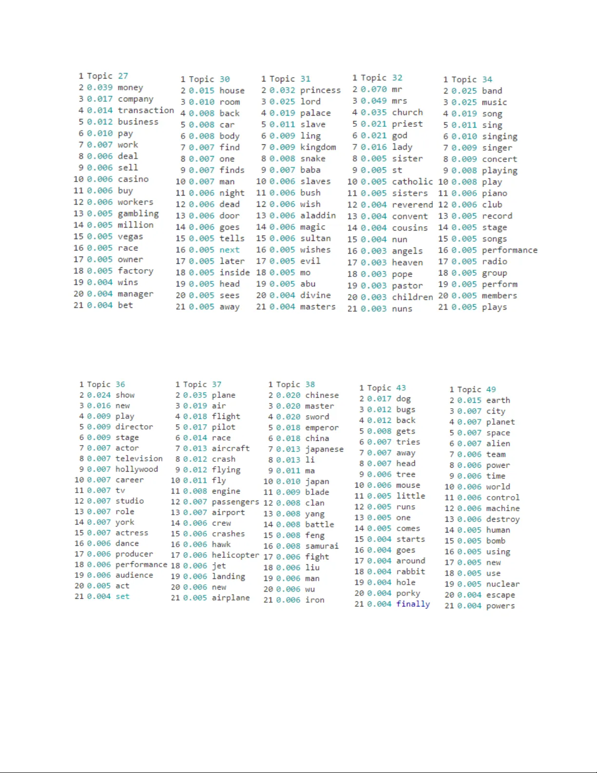
Feature extraction using Latent Dirichlet Allocat ion and Neural Networks : A case study on movie synopses Despoina I. Christou Department of Applie d Informatics University of Macedo nia Dissertation submitte d for the degree of BSc in Applied Info rmatics 2015 to my parents and my siblings … Acknowledgements I wish to extend my deepest app reciation to my supervisor, Prof. I. Refanid is, with whom I had the chance to work personally for the first t ime. I always appreciated him as a professor of AI, but I was mostly inspired by his exceptional ethics as human. I am grateful for the disc ussions we had during my thesis work period as I found them re ally fruitful to gain different perspectives on my future work and goals. I am also indebted to Mr. Ioannis Alexander M . Assael, first graduate of Oxford MSc Computer Science, class of 2015, for all his expertise suggestions and continuous assistance. Finally, I would like to thank my parents, s iblings, fr iends and all other people who with their constant faith in me , they encourage me to pursue my interests. Abstract Feature extraction has gained increasing attention in the field of machine learning, as in order to detect patterns, extract in formation, or predict future obse rvations from big data, the urge of informative features is crucial. The process of e xtracting features is highly linked to dimensionality redu ction as it implies the transformation of the data from a sparse high - dimensional space, to higher leve l meaningful abstractions. This dissertation employs Neural Networks for distributed paragraph representations, and Latent Dirichlet A llocation to capture higher level features of paragraph vectors. Although Neural Networks for d istributed paragraph representations are considered the state of the art for extracting paragraph vectors, we show that a quick topic analysis model such as Latent Dirichlet Allocation can provide meaningful features too. We evaluate the two method s on the CMU Movie Summary Corpus, a collection of 25 , 203 movie plot summaries ex tracted from Wikipedia. Finally, for both approaches, we use K- Nearest Neighbors to discover similar mov ies, and plot the proje cted representations using T-Distributed Stochastic Neighbor Embedding to depict the c ontext similarities . These similarities, expressed as movie distances, can be used for movies recommendation. The recommended movies of this approach are compared with the recommended movies from IMDB, which use a collaborative filtering re commendation approach, to s how that our two models could constitute either an alte rnative or a supplementary recommendation approach. i Contents 1. I ntr odu cti on ................................................................................................................................ . 1 1.1 Overview ............................................................................................................................. 1 1.2 Motivation .......................................................................................................................... 3 2. L aten t D iric hl et A llo cat ion ........................................................................................................... 4 2.1 History .................................................................................................................................... 4 2.1.1 TF – IDF scheme .............................................................................................................. 4 2.1.2 Latent Semantic Analysis (LSA) ...................................................................................... 6 2.1.3 Probabilistic Latent Semantic Analysis (PLSA) ............................................................... 8 2.2 Latent Dirichlet Allocation (LDA) ........................................................................................ 10 2.2.1 LDA intuition ................................................................................................................. 10 2.2.2 LDA and Probabilistic models ....................................................................................... 15 2.2.3 Model Inference ........................................................................................................... 17 2.2.3.1 Gibbs Sampler ........................................................................................................ 18 3. A uto enc od ers ............................................................................................................................. 22 3.1 Neural Networks .................................................................................................................. 22 3.2 Autoencoder ........................................................................................................................ 25 3.3 Backpropagation method ................................................................................................... 27 4. Fe atu r e Re pres en ta tio n ................................................................................................ ............. 31 4.1 Word Vectors (word2vec models) ...................................................................................... 31 4.2 Using Autoencoder to obtain paragraph vectors (doc2vec) ............................................. 36 4.3 Using LDA to obtain paragraph ve ctors ............................................................................. 38 5. C ase Stu d y: Mov ies M ode llin g .................................................................................................. 40 5.1 Movie Database ................................................................................................................... 40 ii 5.2 Preprocessing ...................................................................................................................... 40 5.3 Learning features using LDA ............................................................................................... 41 5.4 Learning features using Autoencoder ................................ ................................................ 42 5.5 K-Nearest Neighbors ........................................................................................................... 43 5.6 t-SNE ..................................................................................................................................... 44 6. M od els Ev alu ation ..................................................................................................................... 46 6.1 Symmetric LDA Evaluation .................................................................................................. 46 6.1.1 Evaluated Topics ........................................................................................................... 46 6.1.2 Dataset Plot ................................................................................................................... 50 6.1.3 Movies Recommendation ............................................................................................ 56 6.2 Autoencoder Evaluation ..................................................................................................... 58 6.2.1 Dataset Plot ................................................................................................................... 58 6.2.2 Movies Recommendation ............................................................................................ 63 6.3 Comparative evaluation of models .................................................................................... 65 7. C on clus ions ................................................................................................................................ 68 7.1 Contributions and Future Wor k .......................................................................................... 68 Appendix A ..................................................................................................................................... 69 Appendix B ..................................................................................................................................... 70 Appendix C ..................................................................................................................................... 71 Bibli ogr aph y ................................................................................................................................... 73 1 Chapter 1 . Intr oduction 1.1 Overview Thanks to the enormous amount of electronic data that is the digitization of old material, the registration of new material, sensor data and both governmental and private digitizati on intentions in general, the amount of data available of all sorts has been expandin g and increasing for the last decade. Simulta neously, the nee d for automati c dat a organiza tion tools a nd sea rch engi nes has become ob vious. Na turally, this has led to an increased scienti fi c interest and activity in related areas such as pattern recognition and dimensionality reduction, fields related mostly to feature extraction. Althou gh the history of text categorizati on dates back to the introduction of co mputers, i t is onl y from t he ea rly 90 ’ s that text categorizati on has become an important part of the mainstream research of text mining, thanks to the increased applica tion-oriente d interest and to the rapid development of more powerful hardware. Categorizati on has successfully proved its strengths in various contexts, such as automatic document annotation (or inde xing), do cument filtering (spam filtering in particular), automat ed met adata generation, word sense disambiguation, hierarchical categorizati on of Web pages and document organization, just to name a few. Probabili stic Models and Ne ural Networks consist t he two state of the art methods to extract features. The efficiency, scalability and quality of document classif ication algorithms heavily rely on the representation of documents (Chapter 4). Among the set-theoretical , algebraic and probabilistic approaches, the vect or spa ce model (TF – IDF scheme in Section 2.1) representi ng documents as vectors i n a vector space is used most widely. Dimensionality reduction of the term vector space is an important concept that, in addition to increasing efficiency by a more compact document representation, is also capable of removing noise such as synonymy, polysemy or rare term use. Ex ample s of dimensionali ty reduction include Latent Semantic Analysis (LSA in S ection 2.2) and Probabilistic Latent Semantic Analysis (PLSA in Section 2.3). Deerwe ster et al. in 1990 [1] proposed one of the most basic approaches to topic modelling, cal led LSA o r LSI. This method is ba sed on th e theory of linear algebra and u ses the bag -of wo rds assumption. The core of the method is to apply SVD to the co -occurrence count matrix of documents and terms (o ften referred to as the term-document matrix), to obta in a reduced dimen sionality representation of the documents. In 1999 Thomas Hofmann [2] suggested a model called probabil istic L atent Semanti c Indexing (PLSI/PLSA) in which the topic distributions ove r words were still estimated from co-occurrence statistics within the documents, but introduced the use of latent topic variable s in the model. PLSI is a 2 probabilistic method, and has shown itself superior to L SA in a number of applications, includin g Information Retrie val (IR). Since then there hav e been an increasing focus on using probabili stic modelli ng as a tool rather than using linear algebra. A more interesti ng approach that can be suita ble for low dimensional representation is the generative probabil istic model of text corpora, namely Latent Dirichlet Allocation (LDA) by Blei, Ng, Jordan [3] in 2003 (Section 2.2) . LDA model s every topi c as a distribution over the words of the vocabular y, and ev ery document as a distribution over the topics, thereb y one can use the latent topic mixture of a document as a reduce d repre sentation. According to Blei et al. [3] PLSI has some shortcomings with regard to overfitting and gene ration of new docume nts. This was one of the motivating factors to propose Latent Dirichlet Allocation (LDA) [BNJ03] , a model that quickly became very popular, widel y used in IR , Data Minin g, Natural Language Processing (NLP) a nd relate d topi cs. Probabilistic topic models, such as late nt Dirichlet al location (Blei et al., 20 03) and proba bilistic late nt semantic ana lysis (Hofmann, 1999, 2001), model documents as finite mixtures of speci alized distributions ov er wor ds, know n as topi cs. An importa nt as sumption unde rlying these topic mo dels is that documents are generat ed by first choosing a document-speci fic distribution over topics, and then repeatedly sele cting a topic from this distribution and drawing a word from the topic s elect ed. Word order is ignored and each document is modelled as a “ bag- of -words ” . The weakness of this approach, howev er, is that word order is an importan t component of document structure, and is not irrelevant to topic modelling. For example, two sentence s may have the same unigram statistics but be about quite different topics. Information about the order of words used in each sentence may help disambiguate possible topics. For further information see Chapter 2. N-gram lang uage models [4] [5] decompo se the probability of a string of text, such as a sentence, or document into a product of proba bilities of indiv idual words given some number of p revious words. Put differently, these models assume that documents are generated by drawing each word from a probability distribution specific to the conte xt consisting of the i mmediatel y preceding words, assuming they use local linguistic s tructu re. As to figure out these features, we us e the Autoenc oder Neural Network ( Chapte r 3) which is highly u sed as a ma chine learning te chnique tha t use s paragraph vect ors t o represent the network input. Paragraph Vectors [6] (see Section 4.2) are closely related to n -grams and are able to ca pture this disadvantage of the bag - of -words models, the linguistic structure. Precisely, paragraph vector is an unsupervised algorithm that learns fixed-length feature representati ons f rom variable-length pieces of texts, such as sentences, paragraphs, and docume nts. Moreover, Neural Network s can represent dimensionality reduction models, when their hidden layer(s) are of smaller size that the input. Precisely, we use Autoencode r Neural Network, because of its structure that assumes the output to have the same size as the input. This charact eristic helps interpreting out data more precisely, as the hidden layer is a compact representati on of the data. For furthe r information see Cha pter 3 and 4. Capturing features, either with a probabilistic model or with a Neural Network, it is important to f in d similaritie s in the extract ed fe atures. K-Nearest Neighb ors is such an a pproach tha t uses cosine dista nce a s a similarity mea sure. Fu rthermore, wi th T-SNE, a n onlinear dimensional ity red uction technique that is well suited for embe dding high-dimensional data into a s pace of two or th ree dimensions we are able to tran sfer the extracted f eatures in the 2-dimensional space, where we can visualize the features in a scatter plot. The representing data captures respective distance similariti es as the KNN does, but in a more huma n friendly interp retable way. F or further informat ion see Chapte r 5 and 6. 3 1.2 Motivation Feature extraction gains increasing attention in the fie ld of machine learning a nd pattern recognition , as the urge of informat ive features i s crucial in or der to detect patterns and extract i nformation . Thinking of recommendation systems, the problem comes to the initial information needed as to recommend the relevant object for our scope. At the beginning we do not have data from users w hile in the following time the user-data ma y be sparse for certain ite ms [7] . Speaking f or movies recommen dation, feature extract ion from mo vie plots con stitutes a wa y for cluste ring relev ant movies as to reco mmend the relevant ones according to their plots, namely their genre. In this thesi s we show that feature e xtraction either from a probabilistic model, such as the state of the art Latent Dirichlet Allocati on, or from a Neural Network, namel y the Autoe ncoder, can constitut e a significa nt base for recommen dation systems . Among different recomme ndation approache s (content-based, c ollaborative filtering and hybrid [8]) , collaborativ e f iltering techniques have been most widel y used (IMDB recomme ndation method) , largely because they are dom ain independent, require minimal , if any, information about user and item features and yet can still achieve accurate predictions [9] [10]. Even though they do manage some prediction, the accuracy of rating predictions is hig hly increased with content information as proved in [7] [11] [12] [13]. Moreover, in [1 4] t he probabil istic topic mo del of LDA i s used on movi e text revie ws to s how that ext racted features from texts can provide additional diversity. Me anwhile, both LDA and Autoencoder can be used as recommendati ons algori thms. Precisely, in conte nt-based and in collaborative filtering recommendation methods, the algorithms used are divided in memory-based and in model-based approache s. Memory- based methods predict users’ prefe rence ba sed on the ratings of ot her simil ar use rs (paragra ph vectors - Autoencoder, See Section 4.2), while model-based methods rel y on a predict ion model b y using Clu stering (i.e. LDA) [15]. In this thesis, we want to testify that LDA and Autoencoder, both used as methods for f eature extraction , present a stonishing movie recommendati ons, rea ffirmi ng that a system which make s use o f conte nt might be able to make predict ions for this mov ie even i n the absence of ratings [1 6]. Moreover, we com pare the two methods with the recommending results of the col laborating filtering process of IMDB a s to discover a comparison amon g them (see Conclu sions, Chapter 7). 4 Chapter 2 2. Latent D irichlet Allocati on Topic modeling is a classic problem in natural languag e processing a nd machine learning. In this chapte r we present Latent Dirichlet Allocation, one of the most successful generative latent topic models deve loped by Blei, Ng and Jordan [3]. Latent Dirichlet Allocation (LDA) can be a useful tool for the statistical analysis of docume nt collections an d oth er discrete data. Specif ically, LDA is an unsupe rvised graphical model whic h can discover latent topics in unlabeled data [17]. This exact characteristic of LDA renders this model pr ior to collaborative models, as for the process of filtering the information of large data sets, the “ many users ” needed for the colla borative process are difficult to exi st from the begi nning. 2.1 History The main inspiration behin d LD A is to f ind a proper modeling framewo rk of the giv en discrete data, namely text corpora in this thesis. The most es sential objective is the dimensionality reduction of our data, so t o ensure efficient backi ngs productive operations, such as information retriev al, clustering, etc. Baeza-Yates and Ribeiro-Neto, 1999 have made significant progress in this field. What IR researche rs pr opose d was to reduce eve ry document in our corpus to a vector of real numbers, each of w hich represents ratios of tallies. Below, we revi ew the three mo st compelling method ologies, whic h preceded the LDA mo del. 2.1.1 TF – IDF schem e Term Frequency – Inverse Document Frequen cy scheme, is the most widely used weighting scheme in the vector space model , which was introduced in 19 75 by G. Salton, A. Wong , and A. C. S. Ya ng [18] a s a model for automati c indexing. Vector space model is an algebraic model for representi ng text documents as vectors of identifiers , for example, index terms, filtered information , etc. TF -IDF scheme is us ed in information fil tering, infor mation retrieval, inde xing and releva nt rankings. In Vector Space Mo del, the corpu s is represente d as follows:            (2.1.1) 5 Here, the documents are represented as finite dimensional vectors, where     󰇛         󰇜 and V the vocabulary size. The we ight   , represent s how muc h ter m   contribute s to the content of the document    and is equal to t he tf-idf va lue. TD - IDF scheme models every document of the corpus as real valued vectors. The weights reflect the contribution to the content of the document. Its value increases pr oportionall y to the number of time s a word shows up in the archive, yet is balanced by the fre quency of the word in the corpus, which serves to adjust for the fact that som e words appear mo re often in general . Term Frequency : t he number of ti mes a term occ urs in a document Inverse Document Fre quency : terms that occur very freque ntly in a document lessen the wei ght of this te rm and relativ ely terms that oc cur rarely inc rease the weight of the correspondi ng term. Ter m Frequency – Inverse Document Frequency (TF - IDF) is the product of two statistics, the Term Frequency and the Inverse Document Frequency . The procedure for implementin g the tf -idf scheme has some min or di fferences co ncurring its a pplication, bu t generally we can assume the tf-idf v alue, as f ollows:              (2 .1.2) where   equals the number of times term t appears in document d, D is the size of the corpus, and   equals the num ber of documents in which t appear s in D [19] . Once, the queries have all been Boolean, implyi ng that documents either match one term or they do not. Answering the problem of too few or too many results, rank-order the documents in a collection with respect to a query was needed. There comes the TF-IDF. Terms with high TF-IDF numbers imply a strong relationship with the document they appear in, suggesting that if that term were to appear in a query for example, the document cou ld be of interest to the user. For in stance if we want to find a term hig hly related to a document, the   should be large, while the   should be small. In that way, the       would be rather large and subsequently   would be likew ise large. This case i mplies that t is an i mportant term in document d b ut not in the c orpus D, so term t has a large discri minatory power. Next i mportant ca se is th e   to be equal to ze ro, with the basi c definition declaring that this ter m occurs in all documents. The simil itude o f two documents (or a docu ment and a query) can be foun d in sev eral wa ys using t he tf-idf weights with the m ost common one the cosine similarity.                           (2.1.3 ) In a typical informati on ret rieval context, given a query and a corpus , the assignment is to find the most relevant documents from th e collection to the query. The first step is to calculate the weighted tf -idf vectors to represent ea ch documen ts and the query, then to compute t he cosine similarit y score for the se vector s and finally ran k and return the document s with the highest sc ore with respect to the query. Disadvantage consist the fact that this representa tion reveals little in the way of inter- or intra-document statistical structure, and the intention of reducing the description length of documents is only mi ldly 6 alleviate d. One way of pena lizing the term weights for a docume nt in accordance with its length can be the document length n ormaliza tion. 2.1.2 Latent Semant ic Analysis (LSA) Latent Semantic Anal ysis ( LSA) i ntroduced in 1 990 by Deerweste r e t a l. [1] is a met hod in Nat ural Language Processing, particularly a vector space model, for extra cting and representing the contextual significance of words by stati stical computations applied to a large corpus. It is also known as Latent Semantic Inde xing (LSI). LSA has proved to be a valuable tool in many areas of NLP and IR and has been used for finding and organizing search result s, s ummarizati on, cluste ring d ocuments, spam filte ring, speech recogniti on, patent searches, auto mated essay e valuation (i.e. PTE tests ), etc. The intuition behind LSA i s t hat words that are clo se i n me aning will occur in similar pieces of text, so by extracting such relationships among words, documents and c orpus we can assume words into coherent passages. Figure 1: Words correlated to cohere nt texts [2 0] As we notice in Figure 1 , a term can correspon d to multiple concepts as lang uages have different word s that mean the same thing (synonyms), words with multiple meanings, and many ambiguiti es that obscure the concepts to the point where people can have a hard time unde rstanding . LSA endeavor s to solve this pr oblem by mapping both words and docum ents into a latent semantic space and transferring t he compa rison in this space . Firstly, a Count Matrix is constructed. The Count Matrix is a word by document matri x, where ea ch i ndex word i s a row and each title is a column , with each cel l representing the number of times that word occurs in the docume nt. The matrices generate d though this step tend to be very large, but also very sparse. In this point we highlight that LSA removes the most frequent used words, known as stop words, give n better results than previous vector model s, a s its vocabular y consist of wo rds that contribute much m eaning. Secondly, raw counts in the matrix at Figure 2, are modified with TF -IDF , as to weight more the rare words and less the most common ones. (See Section 2.1.1 ) Figure 2: Count Matrix [1] 7 Once the count matrix is rea dy, we apply the Singula r Value Decomposition (SVD) method to the matrix . SDM i s a method of dime nsionali ty re duction of our mat rix, namely it recons tructs o ur matrix with the lea st possible informati on, by thr owing away the noise and mai ntaining the strong patt erns. The SVD of a matri x D is def ined as the pro duct of thre e matrices:       (2.1.2 .1 ) D(n*m) = U (n*n) Σ (n*m)V(m* m) (2.1.2.2) , where U matrix represent s the c oordinate s of e ach word in our latent space, the   matrix stands for t he coordinates of each document in our latent space, and the Σ matrix of singular values is a hint of the dimensions or “ concepts ” we need to include. From the Σ matrix we keep only k (number of concepts) Eigen values, a procedure reflecting the major associative patterns in the data, while ignoring the less important influence and no ise. (2.1.2.2) equat ion becomes as follow s: D(n*m) = U( n*k) Σ (k*k) V(k*m) (2.1.2. 3) Figure 3: Dimension Reduction with SVD [1] Lastly, te rms a nd doc uments are conve rted to point s in k-dimensio nal s pace and give n the reduced space, we can compute the similarity between doc-doc, word-word ( synonymy and polysemy), and word- document, by cl ustering our data . Figure 4: Clustering Moreover, in the Information Retrieval field we can find similar document s across languages, after analyzing a base set of trans lated documents and we can also find coherent doc uments to a query of ter ms after its conversi on into the low-dimensional space. A chal lenge to be addresse d in vector space mo dels is twofold: synonymy and polysemy [2]. Synonymy leads to poor recall as they will have small cosine but related, while polysemy concludes to poor precision a s they will have large cosine, but not truly related. LSA as a vector space model cannot retrieve documents coherent to a query unless they have common 8 terms. LSA partially address this, as the query and document are transformed in a lower dimensional “concept” space and are re presented by a simil ar weighte d combination o f the SVD va riables. However, LSA even though it manages to extract proper correlations of words and document s, it handles the text with the bag of wo rds model (BOW), making no use o f word order, syntax and morphology. Another disadvantage is the highly connection with SVD, a computationally inte nsive method, having O(n^2k^3) complexity. Moreover, SVD hypothe sizes that words and documents follow the normal ( Gaussian ) distribution, when a Poison distribution is usually observed. Nevertheless, we can better perform many of the above using Probabilisti c Latent Semanti c Analysis ( PLSA), a preferred method over LSA. 2.1 .3 P rob a bil isti c L at ent S em a nti c An aly si s ( PL SA ) Probabilistic Late nt Semanti c Anal ysis ( PLSA), or Pr obab ilistic Latent Se mantic Inde xing (PLSI), in the field of information retrieval) emb eds the idea of LSA into a probabilistic framework. Contradictory to LSA, which is a linear alge bra method, PLSA sets its foundatio ns in stati stical inference. PLSA o riginated in the domain of statistics in 1 999 by Thomas Hofmann [2], and later on 2003 in the doma in of machine learning by Blei , Ng, Jordan [3] . PLSA is considered as a generative model in which the topic distributions over words are still estimated f rom co-occurrence statistics within the documents as in LSA , bu t the use of latent topic variables is introduced in the model . Pr obabil istic Latent Sem antic Analysis has its most prominentl y applica tions in information retrieval , natural language p rocessing an d machine learning. From 20 12 PLSA ha s been also used in t he bioinformati cs. PLSA practices a generative latent class model to ac complish a probabili stic mixture decomposition. It models every document with a topic-mixture. This mixture is assi gned to the documents in dividually , without a generat ive process a nd the mi xture weights (pa rameters) are l earned by expect ation maximization. The aspect model : The aspect model is the statistical model in which PLSA relies on (Hofmann , Puzicha, & Jordan, 1999). It assumes that every document is a mixture of latent (K) aspects. The aspect model is a latent variable model for co -occurrence data which associates a n unobserved class variable    󰇛        󰇜 with each observa tion, which is the occurrence o f a word in a particula r documen t. Figure 5: PLSA model (asymmetric formulation) [3] Figure 5 ill ustrates t he generative model for the w ord-document co -occu rrence. First P LSA selects a document   , with pr obability 󰇛  󰇜 , then is pick s a late nt variable   with pr obabili ty 󰇛     󰇜 a nd finall y generates a word   with pr obabili ty  󰇛     󰇜 . The result is a joint distribution model, presented in the expression:             󰇛      󰇜           (2.1.3.1) 9 The generation process assume s that for each document    󰇛        󰇜 , for each token position   󰇛     󰇜 we first pick o topic z f rom the multinomial distribution  󰇛      󰇜 and then we choose a term w from the multinomia l distri bution         . The model can be equally paramete rized by a perfectly symmetric model for documents and words . We can see this bel ow:            󰇛󰇜 󰇛    󰇜    󰇛    󰇜 (2.1.3.2) Figure 6: asymmetric (a) and symmetric (b) PLSA representation [2] PLSA as a stati stical late nt variable model introduce s a conditional independe nce assumptio n, namely that d and w are independent set as for the associated latent variable. The parameters of this model are         and  󰇛      󰇜 so according to the above conditional independence assum ption the numbe r of parameters equal s       , namely it grows linearl y with the n umber of document s. The parameter s are esti mated by Maximum L ikelihood, with the Expectation Maximizati on (EM) be the typical procedure ( Dempste r, Laird, & Rubin, 1977). EM substitutes two s teps: the Expectation (E) step where the posterior probabiliti es of the latent variables are calculated and the Maximization (M) step where the parameters are redesigne d. The (E) - step implies to apply the Bayes’ formula in the (2.1.3.1) equation and (M) -step calculate s the expected complete data-log-likelihood, which depends on the outcome of the fir st step as to up date the para meters. ( E) -step:              󰇡   󰇻   󰇢         󰇡   󰇻   󰇢          , (2 .1.3.3) (M)-step : (2.1.3.4) The two steps are alternate d until a termination condition. This can be either the convergence of the parameters or an ea rly stopping, namely the cancel o f updating the parameters whe n their perfo rmance is not improving. PLSA was influe nced by LSA , as a solution for the unsati sfactory stati stical foundation. The main difference between the two is the objective function; LSA i s based on a Gaus sian assum ption, while PLSA relies on the likelihood function of multinomial sampling and aims at an explicit maximization of the predictiv e power of the model. In Figure 7 [2], we notice the difference in LSA’s and PLSA’s pe rplexity i n a colle ction of 1033 documents, clearly revealing PLSA’s predictive supremacy over LSA. As noted in the disadvantag es of LSA in Section 2.1 .2, the Gaussian distribution hardly stands for count data. As for the dimensionality reduction, PLSA per forms it s method by having K aspec ts, while LSA keeps 10 only K singular values for its method. Consequently, when the selection of proper value of K in LSA is heuristic , PLSA‘s mo del selecti on (aspect model) can determine an optimal K maximizing its pr edictive power. Regarding the com putational complexit y of LSA ( O (n^2k^3)) and PLSA (O (n*k*i), with i counting the iterations), the SVD in LSA can be compute d precisely, while EM is an iterati ve method which only affirms to find a local maximum of the likelihood function. Howe ver Hofmann’s experiments have shown that when using regularizati on techniques, as ‘ early stopping’ in order to avoid the overfitting, presente d both in global and local maximums, even a “poor” local maximum in PLSA might performs better than the LSA’s solution . 2.2 Late nt Dirichlet Allocat ion (LDA) Latent Dirichlet Allocation (LDA), a generative probabilisti c topic model for colle ctions of discrete data, is the most representative example of topic modeling and it wa s first presented as a graphical model for topi c discovery by Blei, Ng, Jorda n in 2003 [3] , when they put into question the Hofmann’s PLSI model [2] . Due to its high modularity, it can be easily extended, giving much interest to its s tudy . LDA is also an instant of a mixed membership model [21] , so accordin g to the Bayesian analysis as each document is associate d wit h a distribution, it can be asso ciated with multiple components respectiv ely. LDA as a topic model intends o n detecting the the matic info rmation of large a rchives and can be adapte d as to find patterns in generic data, images, social networks, and bioi nformatics. 2.2.1 LDA intuition Years ago the main issue was to f ind inf ormation . Nowadays , human knowledge and behavior are in high percentage digitized in the web and more precisely in sci entific articles, books, blogs, emails, images, sound , video, and social networks, transferring the is sue on how to interact with these el ectronic archive s each time yet more ef ficiently. Here comes the topic modeling, with LDA the most char acteristi c topic modeling algorithm. Topic Modeling do es not require any prior annota tions or labeling of the archiv es as topic models are able to detect patte rns in an uns tructured collect ion of documents and t o organize these elect ronic archives at a scale that would be inconceivable by human annotation. Topic models as statistical models have their origins to PLSI, created b y Hofmann in 1999 [ 2]. Latent Dirichlet Allocation (LDA) [3] an a melioration of PLSI, is probabl y the most common topic model currently in use as others topic models are generally extension s on LDA. The objective of LDA is to discover short descriptions of the collection’s individual s, reducing the plethora of the initial informatio n into a smaller interpretable space, while keeping the essential statisti cal dependences to f acilita te efficient proces sing of the data. If speaking for text corpora as our collection, Latent Dirichlet Allocation assumes that each document of the collection exhibits multiple topics [3], with the topic probabili ties providing an e xplicit repre sentation of the corpu s. 11 LDA as sumes tha t all docu ments in the collecti on shar e the same set of to pics, but each d ocument e xhibit s those topics with different proportion. We can better understand LDA’s objective in Blei‘s representa tion of the hidden topics in a scientific docu ment in Figu re 8 below: Figure 8: The intuition behind LDA. (Generative process) by D. Blei [17] In Figure 8, w ords from diff erent topics are highlighted with different colors. Fo r example yellow represents words about genetics, pink words about evolutionary life, green words about neurons and blue words about data analysis, declaring the nature of the article and the mixture of multiple topics which is the intuition of the model . LDA as a ge nerative probabilisti c model treats data a s obse rvations tha t ar rive from a generat ive probabilistic process that includes hidden varia bles. These hidden or late nt variables reflect the thematic structure of the coll ection, the topics, with the histogram at right in Figure 8 representi ng the document’s topic distribution. Moreover, the word mixture of each topic is represente d at left, also given the probabiliti es of each word’s e xhibition in eve ry topic. This procedure assumes that the order of words does not necessarily matter. Even though documents would be unreadable with thei r words shu ffled, we are a ble to discover the the matically coherence terms , we are interested a bout (se e Section 2.2.2 about bag of w ords). At this sense, sa me words can be observed in m ultiple topics but with d ifferent probabili ties. Every topic contain s a probability for every word , so even though one word does not hav e high probability in one topic, it might have a grea ter one in another. The main intuition behind L DA as said above is tha t documents exhibit multi ple topics. I n Figure 8, one can notice that documents in LDA are modeled by assuming we know the topic mixture of all documents and the word mi xture of all the topics. Havi ng this knowle dge, the model as sumes that the document at first is empty, then choose a topic from the topic mixture and then a word from the word mixture of that topic, repeating this proce ss until the document is shaped . This exact proce dure is repeat ed for eve ry docum ent in the corpus. This process cons titutes the generative character of the LDA model, namely its attribute of generating obse rvations, give n some hidden variable s. 12 The generative p rocess of L DA can be seen in the following algorithm [22]: Algorithm 1: Generative process of LDA Figure 9: LDA notation The algorithm has no information about the topics. The inferred topic distributi ons are gene rated by computing the hidden structure from the obs erved documents. The problem of inferring the late nt topic proportions is translated to compute the posterior distribution of the hidden variables given the documents. For the generative process of LDA f irst we have to model each document with a Poisson di stribution over the words. T his first step is not presented in the Algorithm 1, but i s considered as known in line 8 and it can also be seen in LDA’s notation in Figure 9 . Second, for each topic we assume the random variable  󰇍   , a dirichlet distributi on of the words in topic k, paramete rized by   , a V-dimension vector of positive real s, summing up to one, t hat is t o be e stimate d. Thi rd, for each document we compute the random variable    , a dirichlet distribution o f th e topics occu rring in docum ent m, parameterized by   , a Κ -dimension v ector of positive reals, summing up to one. Then for each document, the followi ng steps are repeated for every word n of document m: First we identify the topic of the word as a multinomial distribution given    , the topic distrib ution of document m and secondly we choose a term from  󰇍   , the word distribution of the chosen topic in the forwa rd step. These two steps s how that document s exhibit the late nt topics in different 13 Figure 10: graphical model representation of LDA proportions, while each word is drown from one of the topics . Finall y this process is repeated for all the documents in our corpus with the goal to esti mate the posterior ( conditi onal) distribution of the hidden variables by first defining the joint probability distribution of the observed and the l atent rando m variable s. The generati ve process for LDA correspond s to the f ollowing joint distribution of the late nt and the observed variable s for a do cument m: , ( 2 . 2 . 1 . 1 ) (2.2.1.1) where the   are the only obse rvable variables, namely a bag of words organized by docu ment m each time , w ith all the other s being the l atent o nes. E quatio n (2.2.1.1) denotes there a re thre e lev els to the LDA representation . The hyperparameters α and β are corpus level parameters, assum ed to be sampled once in the process of generating a corpus. The variable    are document-leve l variables, comp uted once per document. Finally, the vari ables    and   are word level variables and are sampled once for each word in ea ch doc ument smoothed by p       .an d   are word leve l varia bles and a re samp led once for each word in ea ch document smoothed by p       . The joint distri bution for th e whole corpus i s described by the (2.2.1.2):     󰇍                    󰇡                 󰇍 󰇍     󰇍     󰇢   (2.2.1. 2) The interpretation of the (2.2.1.1) eq uation can be better understood by LDA’s graphical representation, first presente d as such mod el by Blei et al. [3]: LDA as a pr obabil istic graphical model sh ows the s tatistica l assumptions, behind the generative pr ocess described ab ove, which relies on the Bayesian Networ ks. In Figure 10, the boxes plates represent loops. 14 The outer plates represent the documents, while the inner plates represent the repeated choice of top ics and words within a document [3] [2 3]. Moreov er eve ry single circled node decla res a hidden varia ble, while the unique double circled node of w represents and the only o bserved variable , the words of the corpus. Figure 10 illustrates the conditional dependences that define the LDA model. Specifically, the topic indicator    depends o n    , the topic proportions of document m. Futhermore, the observed word  󰇍 󰇍   depends on    , the topic indicator a nd  󰇍   , the word distrib ution of th e topic that    indicates . The choice of the topic assignment   and the choice of n word from the word distribution of topic m,  󰇍 󰇍    are represented as multinomial distributions of    and  󰇍   respective ly. Here, the multinomial distribution is assigned to the Mul tinomial with just one trial. In this case the multinomial distribution is equivale nt to the cate gorical distri bution. In pr obabil ity theory and statistics, a cate gorical dist ribution (also called a "generalized Bernoulli distribution" or, less precisely, a "discrete distribution") is a probability distribution that desc ribes the result of a random even t that can take on one o f K possible outcome s, with the probability of each outcome separately specified. There is not necessarily an underlying ordering of these outcomes, but numerica l labels are attached for convenience in describing the distributi on, often in the range 1 to K. Note that the K-dimensional cate gorical distribution is the most general distributi on over a K-way eve nt; any other discrete distributi on over a size-K sample space is a speci al case. The paramete rs specifying the probabil ities of each possible outcome a re const rained onl y by the fa ct that each must be in the range 0 to 1, and all mu st sum to 1. In the LDA model, we assume that the topic mixture proportions for each document are draw n from s ome distribution. S o, what we want is a distribution on mult inomials. T hat i s, k-tuples of non-negative number s that sum to one. We can represent the topic proporti ons of a document m,     and and the word distributions of a topic k,  󰇍   , as a M-1 topic simplex and V-1 vocabulary simplex repse ctively. As a simplex we assume the geometric interpretati on of all these multinomials. More precisely we assume that the single value s of θ and φ in Fi gure 10 come from a dirich let distribution . A dirichlet distribution is conjugate to the multinomial distributio n paramete rized by a vector α of positive reals with its density function giving the belief that the probabil ities of K rival events are x i given that each event has been observed α i -1 ti mes. I n Bayesian st atisitc s, a dirichlet distribution is used as a prior distribution, namel y a proba bility distribution of a n event we have no evidence about. The representation o f the k -dimensio nal Dirichlet rando m va riable θ and of V-dimen sional Dirichlet ran dom variable φ in the simplex , i s deeper analyzed in Section 5.4. as to understa nd how the conce tration parameters α an d β can influence the results of LDA 15 2.2.2 LDA and Prob abilistic models Latent Dirichlet Allocati on wa s intro duced by Blei et al. [3] a s a probabilisti c gra phica l model. In this Section we describe the basic discipli nes that prevail in the probabili stic models. As descri bed in Section 2.2.1 LDA follows a generative process to discover the hidden variables by ascribing statistic al inference to the data. Specifically, using stati stica l i nference we can inv ert the gene rative process a nd obtain a pr obability distribution of a document’ s topic mixture . These principle s – generative processes, hidden variables, and statistical inferen ce – are the foundati on of probabi listic models [24] . Probability theory holds the foun dations as to model our beliefs about different possible states of a situation, and to re -estima te them when new evidence comes to the forefront. Even though probability theory has existed since the 17th century, our ability to use it effectiv ely in large problem s involving many inter-relate d variable s is fairly rece nt, an d is due to the development of a f ramework known a s Probabil istic Graphical Models (PGMs). LDA constitut es the state of the a rt such model and is subsequent t o the Probabilistic L SA. Both LDA and PLSA, as most of the probabilistic models rely on the “bag of words” assumptio n that is the order of words is irrelevant. Many words, especial ly nouns and verbs that only seldom occur outside a limited number of c ontexts, have one speci fi c meaning or at least only a few, not d epending on the pos ition in the text. In this basis the b ag - of -words assumption captu re s the topic mixture and can effect ively describe the topica l aspects of the doc ument collection . This “bag of words ” assumpti on equals the exchange ability property. Exchangeabil ity property assumes that the joint distribution is invariant to permutation. If p is a permutation of t he integers from 1 to N , we can say that a finite set of random variable s 󰇝        󰇞 is said to be exchangea ble [25]: p (        ) = p((  󰇛󰇜     󰇛󰇜 )) (2.2 .21) where π ( ∙ ) i s a permutatio n function on t he integers {1… N}. Respectivel y, an infinite sequence of random variables i s in finitely exchangeable if eve ry finite subsequenc e is exchangeable . De Finetti’s representation theorem [26] states that the joint distribution of an infinitely exchangeable sequence of random variables is as if a rando m param eter were drawn from some distribution and then the random varia bles in question were indepe ndent and identical ly distribute d, c onditioned on that parameter. Note that an assumption of exchangeability is weaker than the assumption that the r andom variables are independe nt and identically distributed. Rather, exchangea bility essentially can be interpreted as meaning “ conditi onally i ndependent and i dentically distributed ” , w here t he co nditioning is with respect to an un derlying latent pa ramete r of a probabi lity distribution. That is to say t hat the conditional probabi lity distribution  󰇛          󰇜    󰇛     󰇜    is ea sy to expre ss, while the joint dist ribution usually cannot be decomposed. 16 We are going to examine LDA respectively to its precedent pr obabili stic model PLSA as to better view the process of the probabilities models in time, as also to highlight the advantages of L DA over the other s similar models. First, the exchangeabil ity property was exploite d in PLSA only on the leve l of words. As on e can argue that not only words but also documents are exchangeable , a pr obabilistic model should capture the exchangeability of both words an d documents . LDA ev olved from PLSA by extending the exchangea bility property to the le vel of documents by applying Dirichlet priors o n the multinomial distributio ns     󰇍   . LDA assumes that words are generated by the fixed conditional distribution s over topics with those topics be infinitely exchangeable within a document. By de Finetti’s theorem, the prob ability of a sequence of words and topics must ther efore have the form: p(w, z ) =  󰇛󰇜󰇛   󰇛     󰇜  󰇛      󰇜   󰇜  (2 .2.2.2) where θ is the rand om para meter of a multino mial over topics . As noted by Blei, et al. [3] “ PLSI is incomplete in that it provides no probabilistic model at the level of documents. In PLSI, each document is represented as a list of numbers (the mixing proporti ons f or topics), and there is no generative p robabili stic model for these numbers. ” Latent Dirichle t allocati on models the documents as f inite mixture s over an underlying set of latent topics with specialized distributions over words which are inferred from correlations between words, independently of the word order ( bag of words). Namely, LDA appends a Dirichlet prior on the per-document topic distributi on as to address the criticized ine fficiency of PLS A inferred above. Let notice the probabil istic graphic al model of the two models to infe r the differe nces. Figure 11: graphical representation of PLSA (at left) and LDA (at right) In PLSA   is a m ultinomial random va riable and t he model learns the se topic mixtures only for the training documents M, thus PLSA i s not a fully generativ e model, particularly a t the level of docume nts, since there is no cle ar soluti on to as sign pro bability to a prev iously unsee n docu ment. This lead to the con sequence of the linear growth of the nu mber of para meters to be estimated with the numbe r of training documents . The parameters for a k-topi c PLSA model are k multi nomial distrib utions of size V and M mixtures over the k hid den to pics. This gi ves kV + kM parameters a nd thus grows linearly in M. The li near growt h in parameters impli es that the model is prone to over fitting. Even though tem pering heuristic is prop osed by 17 [2] to smooth t he paramete rs of the model for acce ptable predict ive perfor mance, it ha s been shown that overfitting can occ ur even then [2 7]. LDA as noted in [3] overcomes both of these problems by treating the topic mixture weights as a k parameter hidden rando m variable sampl ed from a Diric hlet distribution, applicable a lso for unseen documents. Furthermore , the number of paramete rs is k + kV in a k -topic LDA model, which do not grow with the size of the traini ng corpus, thereby avoids overfitting. Moreover , the count for a topic in a document can be much more i nformative than the count of indiv idual words belonging to that topic. Illustrating the se differences in a la tent space, we can see how a document is geomet rically represe nted under each mode l. Each document is a distribution ov er words, so below we ob serve ea ch distribution a s a point on a (V- 1) simplex, name ly document’ s word simplex . The mixture of unigrams model in Figure 12 maps each corner of the word simplex to the wor d probability, equal to one. Each topic corner i s then chosen randomly and all the words of the document are drawn from t he distribution corresponding to t hat point. In PLSI topics are the mselve s drawn from a document- specific distribution, denoted by spots. LDA though, draws the topics from a distribution with a randomly chosen parameter, different for every document , denoted by the contour lines in Fi gure 12. Figure 12: The topic simplex for three topics embedded in the word simplex for three words [20]. 2.2.3 Model Inferenc e In LDA, d ocuments are repre sented as a mi xture o f topi cs and each topic has some particular probabil ity o f generating a set of words. T hus, LDA assumes data to arise from a generative process that includes hidden variables. This generative process defines a joint probabil ity distrib ution over both the observ ed and the hidden random variables, transferring the inferential problem to compute the posterior distribution of th e hidden variables giv en the observe d variables, which are the documents. The posterior dist ribution is :  󰇛          󰇜                    (2.2.3. 1) The numerator is the joint distribution of all the random variables, which can be easily computed for any setting of the hidden variables. The denominator is the marginal probability of the observations, which is the probability of seeing the observed corpus under any topic model. Posterior distribution cannot be directly comp uted. Thus, to solve the problem we need approximat e inference algorithms as to form an 18 alternati ve distribution which is clo se to the posterior. Such al gorithms are divided in the sampling based algorithms and the variational algorit hms . Samplin g based algorithms collect samples from the posterior to approximate it with an empirical distribution, while variational methods place a parameterized class of di stributions over the hidden structure and then find the member of that class that is closest to the posterior, using Kullbac k-Leibler divergence [28]. Thus, the infere nce problem is turned into an optimization proble m. The most popular appro ximate posterior inference algorithms are the mean field variational method by Blei [3], the ex pectation pr opagati on b y Minka and Laffe rty [29] and Gibb s Sampling [30], with many others or extensions o f the above. 2.2.3.1 Gibbs Sampler Gibbs sampling is c ommonly u sed a s a method of statisti cal i nference, e specially Bayesian inference . Gib bs sampling is named after the physicist Josiah Willard G ibbs, in re ference to an analogy between the sam pling algorithm and statistical physics. The algorithm was described by the Geman brothers in 1984 [31], some eight decades after Gibbs’s death. Part o f the Gibbs Sa mpler work presented is based on the thesis of Istvá n Bíró [32]. Gibbs sampling is applica ble when the joint distri bution is not known surely or is difficult to sample from the beginning, but the conditional distribution of each variable is known and i s easy to sample from. The Gibbs sampling algorithm generates an instance from the distribution of each variable in turn, conditional on the current values of the othe r variable s. It can be shown that the sequence of samples constitutes a Markov chain, and the st ationary distribution of that Markov chain is just the recherche joint distribution [33]. Subsequently, Gibbs Sampler or Gibbs Sampling is an algorithm based on Markov Chain Monte Carlo (MCMC) simulation. As noted in [33] , MCM C algorithms can simulate high-dimensional probability distributions by the stationar y behavior of a Markov chain . The process generates one sample per transmition in the chain. The chain starts from an initial random sta te, then after a burn-in period it stabilizes by eliminating the influence of initialization parameters. The MCMC simulation of the probability distribution p(   ) is as follows: dimensions x i are sampled alternate ly one at a time, conditioned on the values of all other dimensions denoted by  󰇍 󰇍   = 󰇛                 󰇜  which is: 1. Choose dimension i (random or by cyclical permutation) 2. Sample   from p 󰇛     󰇍 󰇍   󰇜 As stated above the c onditional distribution of each variable is known and can be calculated as follows: (2.2.3.1.1) 19 In order to construct a Gibbs sampler for LDA, one has to estima te the probabil ity distribution  󰇛     󰇍 󰇍  󰇜 for  󰇍 󰇍         󰇍 󰇍       , w here N denote s the se t of wo rd-positions in the corpus. This distribution i s dir ectly proportional to t he joint dis tribution: (2.2.3.1. 2) This joint distributio n cannot be infer red because of the denominator, which is a summation over   terms. This is why we use Gibbs Sampling, as i t require s only t he full conditi onals p 󰇛     󰇍 󰇍     󰇍 󰇍  󰇜 as to infer p 󰇛     󰇍 󰇍  󰇜 . So, first we have to estimate the joint distribution: (2.2.3.1. 3) Because the first term i s independent of   due to the conditi onal independence of  󰇍 󰇍  and   given  󰇍 󰇍  , while the second term is independe nt of   . The element s of the joint distribution can now be managed inde pendently. The first term can be obtaine d from p 󰇛  󰇍 󰇍      󰇜 , which is simply: (2.2.3.1 .4) The N words of the corpus are observed according to independent multinomia l trials with parameters conditioned on the topic indices   . In the second equ ation we split the product over words into one product over topics and one over the vocabulary, separating the contributions of the topics. The term    denotes the nu mber of ti mes that term t has been obs erved wi th topic z. The distr ibution p   󰇍 󰇍       󰇍   i s obtain ed by integrati ng over Φ, which can be done using Dirichlet integrals with in the product over z , as can be seen bel ow: (2.2.3.1.5 ) The topic distributi on p 󰇛      󰇍  󰇜 can be derived fro m p 󰇛      󰇜 : (2.2.3.1.6 ) 20 where    refers to the docum ent word    belongs to a nd   refers to the n umber of tim es that topic z has been observe d in document m. Integrating o ut Θ , we obtai n: (2.2.3.1.7 ) Consequently, the joint distributi on becomes: (2.2.3.1.8 ) Now, by using (2.2.3.1.8) equation we can determ ine the update equa tion for the hidden variable : (2.2.3.1.9 ) where the super script   denotes that the wo rd or topic with index  is excluded from the corpus when computing the co rresponding cou nt. Note that only t he terms of t he product s over m and k contain the index  , while all the others are cance lled out. Having this k nowledge we c an calculate the value s of Θ , Φ from the giv en state of the Mar kov chain as a re the current samples of p 󰇛     󰇍 󰇍  󰇜  This can be done as a post erior estimation, by predicting the distribution of a new topic-word pair (   = k ,  󰇍 󰇍  = t) that is observed in a document m, given state 󰇛     󰇍 󰇍  󰇜  21 (2.2.3.1.10 ) Using the deco mposition in ( 2.2.3.1.10 ), we can inter pret its first facto r in the first line as    and its second factor as    , hence: (2.2.3.1.11 ) (2.2.3.1.12 ) Gibbs Sampler algorithm, using (2.2.3.1.9 ), (2.2.3.1.11), and (2.2.3.1.12) equations can approximate and infer the initial wa nted poste rior distribution. Moreove r, we should state so me keys about Gi bbs sampling algorithm. During the initial stage of the sampling process namely the burn-in period [30], the Gibbs samples have to be discarded because they are poor estimates of the posterior. After the b urn-in period, the successive Gibbs samples start to approximate the target pos terior of the topic assignments. To get a representative set of samples from this distribution, a number of Gibbs samples are saved at regularly spaced intervals , to prevent correlati ons between sam ples . 22 Chapter 3 3. Autoenc oders Autoencoder, Au toassocia tor or Diabolo network is a special sort of artificial neural networks. Neural Networks as stated by W. McCulloch and W. Pitts [34] are inspired by biological neural networks and they are used to e stimate or approximate fun ctio ns gi ven large data as input, generally unknown. Neural networks are adaptive to these inputs and subseq uently capable of learning [20]. In this chapter after a review to the neural ne tworks, we present Autoencod er, repre sented as a feedfo rward neu ral net most of the times, as a method for dimensionality reduction and feature extracti on. More precisely, the enco der network is used during both training and deployment, while the decoder netw ork is only used during training. The purpose of the encoder netw ork is to discover a compressed representation of the giv en input. In the next chapter s we are going to apply both LDA (described in Chapter 3) a nd Autoencoder o n a movie database as to compare the two methods in their results to dimensionality reduction and feature extraction. The autoe ncoder i s an unsupervised learning algorit hm with the aim to rec onstruct the input i n the outp ut through hi dden la yer(s) of lower dimension. T his compre ssed repre sentation of the data leads to a representation in a reduced space and renders the model capable of discovering latent concepts through our data, w hich is exactl y what we want to capture. Moreover, this exact characteristic, accordingly to LDA, gives interest to ob serve its result s respecti vely to these of collaborativ e filtering models ( see Section 6 ) . 3.1 Neural Networks Neural netwo rks use learni ng algorith ms that are ins pired by the procedu re that our brain learns , but the y are evaluated by how well they work for practical applications s uch as speech recognition, object recognition, image retrieval and the ability of recommendation. Neural networks, f irst described by W. McCulloch an d W. Pitts [34] as a possible approach for AI applications , is a system consisti ng of neurons and adapti ve weights which represent the conceptual connections between the neurons, that are refined through a learning algorith m, c apable of approximating the non-linear functions of their input s. These weight-va lues comprise the flexible part of the neu ral network an d define its beha vior. With appropriatel y 23 network functions, various learning assignments can be performed by minimizi ng a cost function over the network function. Below we can see the simpl est possible neu ral network , the ‘single ne uron’ [35] [36]: Figure 13: 'Single neuron' This "neuron" is a computa tional unit that takes as input x 1 , x 2 , x 3 (and a +1 intercept term), and outputs   󰇛  󰇜   󰇛    󰇜   󰇛        󰇜    , where     is called the activati on function . Neural Networks use basic functions that are nonlinear functions of a linear combi nation of the input s, as stated b y Bi shop [ 20]. Su bsequently, as to from a ba sic neural network model, first we have to co nstruct M linear combination s of the input s        : (3.1.1) where      and (1) superscript denoted the first layer of the network. The   parameter is the weight of the input, while the   represents a bias. Finally,   represents the activation. Each activation is then transfor med via a nonli near activa tion function h (·), usual ly chosen to be a sigmoidal fu nction: (3.1.2) The next layer of the neural net i s the linear com bination of all   ,       (3.1.3) The output is the transformation of each   through a pr oper activati on function, chosen accordingly to the nature of our data. Let σ be the final activa tion function k output is presente d as: (3.1.4) with the overal l network re presented bel ow: (3.1. 5) 24 Figure 14 : Sigmoid (left) and tanh (right) activation functions [20] As an act iv atio n f un ctio n w e usually use the sigmoid o r the hyperbolic tange nt (tanh) functions.  󰇛  󰇜     (3.1.6)   󰇛  󰇜           (3.1 .7) The tanh(z) function i s a resca led version of the sigmoid, and i ts output range is [−1, 1] i nstead of [ 0, 1]. The functions take as in put the weighted sum α , of the values coming from the units connected to it. Note that the o utput values for the σ function range betw een but never ma ke it to 0 and 1. This is because   is never negative , and the denominator of t he fractio n tends to 0 as α gets very big in the negative direction, and tends to 1 as it gets very big in the positive direction. This tendency comes easily as the middle ground be tween 0 and 1 is rarely see n because of the sharp (nea r) step in t he function. Beca use of it looking like a step function, we can think of it firing and not -firing as in a perceptron: if a positive real is input, the output will generally be close to +1 and if a negative real is input the output will general ly be close to - 1. In general, a network function linked to a neural network declares the relationship between input and output layers, paramete rized by the weights. By findi ng out proper network functions, various learning tasks can be per formed by minimi zing a cost function ove r the network function t hat is the weights . A neural network is put together by linking many of our simple "neurons," s o that the outp ut of a neuron can be the input o f another. For example, here i s a smal l neural networ k Figure 14 illustrates a three layer neural net, where x denotes the input layer, y the output layer and the middle layer of the nodes, z, is the hidden layer, we are mainly interested in this thesis, as it represents the representation of our data in a lower dimension space. The shaded nodes represent the biases a nd are not considered a s inputs. Moreover, this is a feedforward neural network. Thus, the information ‘ tr avel s ’ only one directi on . Figure 15: 3-layer neural network [20] When s peaking for a feedf orw ard neur al ne two rk , namely a neural net whose info rmation move in one direction and do not shape any direc ted loops or cycles, by repeating (3.1.1) and (3.1.2) equations we can 25 form a neural netw ork with multiple hidden layer s. Of cour se, neu ral nets ca n hav e more tha n one o utputs as seen in Figure 15 . Multilayer feedf orward neural networ ks can be used to perform fea ture learning and predict ion, si nce the y learn a representati on of their input at the hidden la yer(s), which is subse quently used for classification or regression at the o utput lay er. 3.2 Autoencoder Autoencoders or Auto associator s are a s pecial kind of a rtificial neural networks and provide a fundamenta l paradigm for un supervised lea rning. They we re first int roduced in 1986 by Hinton et al. [37] to address the problem o f backpr opagation ( See Section 3.3) without a teacher", by using the input data to avoid the need for having a teacher and are later related to the concept of Sparse Coding, presented by Olshausen et al. [38] in 1996. T heir input and output layer have the same size and the re is a smaller hidden laye r in between. Autoencoder t ries to reco nstruct the i nput vect or in th e output layer with as much accu racy by learning to map the input to itself ( auto-encode r) in a lower dimension space. Thus, the network is evaluated by evaluat ing the input through the hidden layer to the output layers. Because the goal is to reconstruct the input-vector in the output layer as precisely as possible , the network is back -propaga ted with the error between the reconstructi on and the original pattern. The smaller sized hidden layer has to r epresent the larger input dat a. Therefore, the s ystem learns a compressed rep resentation of the data. The activation of the hidden layer p rovides a compre ssed repre sentation of t he data, the encodin g of the data. More recently , autoenco ders have come to the foref ront in the dee p archite cture of neural networks, a s i f put one on top of each other [39], they create stacked autoencoders capable to learn deep networks [40] [41] . These deep archite ctures are s hown to present gre at results on a numbe r of challenging cla ssification and regressio n problems. Autoencoder, in its sim plest repre sentation is a feedforw ard, non- recurrent neural network, very si milar to a multilayer perceptron. Th e difference is that in Autoencoder the output layer is of the same size as the input layer is, so instead of training the neural net to predict s ome target value ‘y’, the autoencoder is trained to reconstr uct its ow n inputs (auto-enco der). The framework of the Auto encoder as represente d by Baldi [42]: Figure 16 i llustrates the gene ral architecture behind an Autoenco der neural net that is defined by n, p, A , B, X, Δ , F , G. F repre sents the input/output layer denoted as a    ve ctor and G declares the hidden layer, the bottle neck, denot ed as   vector, wi th n , p be positiv e intege rs. A is a transformation class from   to   , B is a similar class from   to   .    󰇝        󰇞 is a set of m training vectors in   and Δ is dissimilarity or di stortion fu nction defined ove r    Figure 16: Autoencoder ’ s architecture Given these tu ples, the co rresponding problem is to fin d        that minimiz e the overall error (distortion) function: (3.2.1) 26 The difference with a multil ayer percept ron whe re the external targe t   a re con sidered as different to the input x, can be be tter understand below, with the mi nimization proble m become as follows: (3.2.2) During the training p hase of eve ry neu ral network, the weights (and hence F) are successiv ely modified, vi a one of several po ssible algorit hms, in order to minimiz e E. Generally there are two options for the Autoencoder network. Mainl y when we refer to an Autoe ncoder neural netw ork we a ssume tha t the layer of the hidden nodes, often referred as bottle neck, (Thompson e t al., 2002), are of s maller dimension than the input and output layer. So, in Figure 16 , we can see precisely this with p