Quantifying information transfer and mediation along causal pathways in complex systems

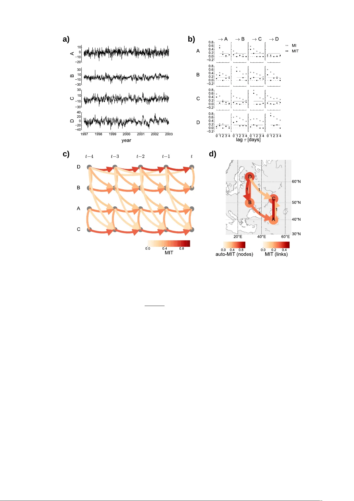
Quantifying inf ormation transfer and mediation along causal pathways in complex systems Jakob Runge P otsdam Institute for Climate Impact Resear ch, P .O. Box 60 12 03, 14412 P otsdam, Germany Department of Physics, Humboldt University , Newtonstr . 15, 12489 Berlin, Germany (Dated: March 21, 2016) Measures of information transfer hav e become a popular approach to analyze interactions in complex sys- tems such as the Earth or the human brain from measured time series. Recent work has focused on causal definitions of information transfer aimed at decompositions of predictiv e information about a target variable, while excluding effects of common drivers and indirect influences. While common driv ers clearly constitute a spurious causality , the aim of the present article is to dev elop measures quantifying different notions of the strength of information transfer along indirect causal paths, based on first reconstructing the multi v ariate causal network ( T igramite approach). Another class of nov el measures quantifies to what extent dif ferent intermediate processes on causal paths contribute to an interaction mechanism to determine pathways of causal informa- tion transfer . The proposed framework complements predictiv e decomposition schemes by focusing more on the interaction mechanism between multiple processes. A rigorous mathematical framework allows for a clear information-theoretic interpretation that can also be related to the underlying dynamics as proven for certain classes of processes. Generally , ho wev er , estimates of information transfer remain hard to interpret for nonlin- early intertwined complex systems. But, if experiments or mathematical models are not av ailable, measuring pathways of information transfer within the causal dependenc y structure allo ws at least for an abstraction of the dynamics. The measures are illustrated on a climatological example to disentangle pathways of atmospheric flow o ver Europe. I. INTR ODUCTION The a vailability of vast amounts of time series data from such complex systems as the Earth or the human brain and body has gi ven rise to a plethora of time series analysis meth- ods aimed at understanding interactions between regions or subprocesses in these comple x systems. Of a particular in- terest are methods to quantify some notion of information flow or information transfer within the complex system. In neuroscience [1] and climate research [2, 3], such interpreta- tions ha ve often been based on pure pairwise correlation anal- yses. But to wards measuring information transfer, the method should, firstly , be general enough to include also nonlinear as- sociations. This can be achieved in an information-theoretic framew ork with measures such as mutual information (MI) [4]. Secondly , networks reconstructed from pairwise mea- sures of association (be it cross-correlation or MI) do not al- low to assess the propagation of information or hypothetical perturbations in a causal sense: For example, an interaction like X ← Z → Y would imply that X and Y are correlated ev en though no perturbations originating in X can actually reach Y , or vice versa. An important step to wards deeper insights has, therefore, been achiev ed by methods that are capable of inferring a statistical notion of directionality or ev en causal interactions which have been applied to the climate system [5 – 10], the human brain [11 – 13], and to disentangle cardiov ascular pro- cesses [14–16], among others. Causal associations between subprocesses can be visualized as links in a complex interac- tion network. A full causal reconstruction of a link X → Y can only be achieved under the in most cases unrealistic as- sumption that all possible other influences on X and Y can be included in the analysis [17, 18], or if the system can be ex- perimentally manipulated within Pearl’ s causal effect frame- work [19]. Usually , it is impossible to exclude all other influ- ences and large complex systems can typically not be easily experimentally manipulated. Causal inference based on data- analysis methods, therefore, provides only a first step and the term “causal” can then only be understood to be meant relati ve to the system under study , i.e., the processes that comprise the nodes of the network. T wo tasks need to be addressed to measure a causal notion of information transfer from time series of complex systems: 1. Reconstructing the causal network, 2. Quantifying causal information transfer . In this article we will focus on the quantification part, the reconstruction problem has been addressed by the author in Ref. [20]. As further revie wed below , previous works have mainly considered a decomposition of the predictiv e informa- tion in direct driv ers of a process Y . In the present article, we ask a different question: Ho w does information originat- ing in a process X propagate also on indir ect paths through the causal interaction network? How strong is it and which intermediate processes on causal pathways are contributing to such a mechanism? The paper is organized as follows: In the remainder of this introductory section, we revie w recent approaches to measur- ing information transfer in comple x systems and sketch the basic idea underlying the present approach. In Sect. II we recall basic concepts of information theory and in Sect. III in- troduce the concept of time series graphs as the causal basis of the present approach. In Sect. IV we introduce the no vel measures based on time series graphs to quantify interactions along paths and mediation and distinguish them from trans- fer entropy-related approaches. In Sect. V we extensi vely an- alyze the measures with analytical and numerical examples and provide theorems that foster a more rigorous mathemati- cal and dynamical understanding to facilitate the interpretabil- ity of the proposed measures. Section VI discusses the theo- 2 retical results and relation to linear measures of causal effect in Pearl’ s frame work [21], and gi ves an outlook to applica- tions of the novel measures in comple x network theory . Fi- nally , Sect. VII giv es an illustrativ e application to climato- logical time series and Sect. VIII concludes the paper . The appendix contains proofs of the theorems. A. Quantifying causal information transfer Compared to the first task of detecting causal interactions, more or less a binary question, the second task of quantifying causal information transfer is much more ambiguous to define in a universal way which has led Smirnov [22, 23] to question the goal of assessing a “causal coupling strength” and instead measure “how the coupling manifests itself in the dynamics” in an interventional-ef fect causal framework as proposed by Pearl [19]. In Ref. [24] the term ‘information transfer’ is ev en distinguished from ‘information flo w’ where the latter is meant in a causal sense based on interv entions. This frame- work, howe ver , necessitates either to experimentally manipu- late the system, or to have a mathematical model to perform “virtual interv entions”. T o some extent causal effects can also be extracted if the time series cover the whole state space or attractor of the complex system [22] such that virtual inter- ventions can be drawn ‘randomly’ from the stationary distri- bution. In a mathematical model the strength of a coupling mechanism can often be related to model coefficients and a plethora of methods exists that implement the model-based concept of Granger causality [17]. These range from classical linear autore gressi ve models in the form of the dir ected tr ans- fer function [25 – 27], to slightly less restrictiv e approaches such as partial dir ected coher ence using spectral estimators [28 – 32], e xtended Gr anger causality with local linear embed- dings in phase space [33], or kernel estimators [34], to name just a few . All these approaches still in volv e strong assump- tions about the dependencies and share the problem that the model might be misspecified. This implies that the model may not adequately represent important interactions such as the complicated interplay between El Ni ˜ no Southern Oscil- lation and the Indian Monsoon in the climate system [35] or neural interactions where even a fully physical model is lack- ing. If it is not possible to measure “ho w the coupling manifests itself in the dynamics”, information-theoretic quantifiers can at least help to measure “how the causal coupling manifests itself in the exchange of entropy between the subprocesses” in an information-theoretic framework capturing almost any form of statistical association. Here ‘causal’ is meant rel- ativ e to the observed process as discussed above. This ap- proach aims to distinguish dif ferent contrib utions based on the Markovian conditional independence structure of the multi- variate process as an abstraction of the dynamics. There are few works considering multiv ariate definitions of information transfer and their interpretation. In Ref. [36], the central concept is to decompose the predicti ve informa- tion about the next time step of a subprocess Y into the MI between Y and its o wn past as the information stor - age , the partial transfer entr opy from another subprocess X , and the TE between Y and the remaining process. In Refs. [37, 38] another decomposition is proposed to detect redundant and synergetic contributions of dri ving v ariables. Liang [39, 40] presents a rigorous approach based on the un- derlying Langevin description of a system to define the contri- butions of internal and external dri ving to the e v olution of the entropy of a subprocess Y . This approach is, howe ver , based on the knowledge of the deterministic-stochastic equations of the system, b ut in principle it can also be estimated from time series alone in volving numerical optimization problems. In Refs. [41, 42] an idea is described that is similar to the present approach in that there the question of quantifying the strength of links is seen as a second step based on the kno wn causal network. A y et al. [41] address the problem from an inter- ventionalist perspective using Pearl’ s do-calculus [19] which we do not further discuss here since we assume the process to be not manipulable. Janzing et al. [42] define the strength of a link X → Y by considering the thought experiment of an attacker ‘cutting the link’ and feeding in the distribution of X as an input, arriving at a measure that is not a conditional mutual information anymore, which we use here to measure the transfer of information. Also, the authors state that it is difficult to quantify also indirect effects in their framework. In general, there are different ways to define measures and different research questions demand dif ferent properties. B. The idea of momentary information The approach to measures of causal information transfer formally introduced in Sect. IV is based on the fundamen- tal concept of source entr opy , also termed the entr opy rate [43, 44], and was introduced for the special case of biv ariate ordinal pattern time series in Ref. [45]. Consider a symbol- generating process X . At each time t a realization x t is gen- erated. Now the source entropy of X t measures the uncer - tainty about x t before its observ ation if all former observ a- tions ( x t − 1 , x t − 2 , . . . ) are known (entropies will be formally introduced in Sect. II). For a completely deterministic non- chaotic system the source entropy will always be zero, but for a real world process there will always be some uncer- tainty stemming from dynamical noise . This type of noise is to be distinguished from observational noise which usually contaminates each measured time series [46], but has no effect on the dynamics of the process. Dynamical noise might occur due to unresolv ed smaller-scale processes and can be modeled by including a random v ariable in the system. More formally , consider a subprocess X of a multiv ariate process X with in- finite past X − t = ( X t − 1 , X t − 2 , . . . ) , that is described by the discrete-time equation X t = f  Z 1 ,t − τ 1 , Z 2 ,t − τ 2 , . . . , η X t  , (1) with some arbitrary function f of other subprocesses at past times Z 1 ,t − τ 1 , Z 2 ,t − τ 2 , . . . ∈ X − t and the random part subsumed under η X t . The uncertainty of an outcome x t will on average be reduced if a realization of the past 3 Figure 1. (Color online) Consider a realization of dynamical noise η X driving subprocess X as a perturbation. Coupling mechanisms along dif ferent causal paths (black lines) transform such a perturba- tion, and the total effect on Y some time later can also depend on ho w intermediate processes nonlinearly interact with each other as shown in Sect. V B. The central idea of the momentary information trans- fer measures presented in this article is to information-theoretically quantify the general effect of such perturbations and isolate it from common drivers in the past such as Z 2 , but also Z 1 and the past of X . T o also quantify how much intermediate processes such as ( W 1 , W 2 ) on causal paths mediate information, it will also be im- portant to exclude common dri vers lik e Z 3 . Z 1 ,t − τ 1 , Z 2 ,t − τ 2 , . . . is known. But for non-zero η X t there will always be some “surprise” left when observing x t . This surprise giv es us information and the expected information here is the source entrop y H ( X t | X − t ) of X . If the dynam- ical noise η X t occurs additi vely in Eq. (1), then H ( X t | X − t ) = H ( η X t ) . Due to measurement errors or observational noise  , we will in general not be able to estimate the source en- tropy alone, b ut only H ( X t +  X t | X − t +  X − t ) . Even assuming a perfect measurement apparatus for a deterministic dynami- cal system without dynamical noise, the entrop y rate h symb – since it is computed by creating a symbol sequence from a coarse graining in phase-space – depends on some resolution parameter r . Then the limit lim r → 0 h symb might exist and is called the K olmogor ov-Sinai entr opy . If this limit is finite and larger than zero, the system is called chaotic. But here we study stochastic, discrete time processes because the finite set of measured v ariables of a complex system like the Earth will nev er perfectly describe the full system’ s state and all remain- ing processes contrib ute to dynamical noise (implying that the K olmogorov-Sinai entrop y div er ges). While the focus in Refs. [36, 37] and related works is on de- compositions of predictive information on the basis of transfer entropy as an information-theoretic generalization of Granger causality , the concept here is more similar to Sims causality , see, e.g., [47], which takes into account not only direct, but also indirect causal effects. Sims causality is based on mea- suring to what extent X at time t helps in predicting Y at times t 0 > t in the future excluding the past of X and also the present of all other processes, i.e., X − t +1 = ( X t , X t − 1 , . . . ) . In model (1) excluding the past essentially isolates the dynam- ical noise η X t and our goal is now to quantify the information transfer emanating from η X t into the future (Fig. 1). W ith this central idea we define two pairs of measures for two purposes: (1) to quantify the information transfer be- tween tw o causally linked processes and along causal paths and (2) the mediation of intermediate processes. For each of these tasks we define two measures quantifying different no- tions of information transfer: Both ha ve in common the abov e idea to extract information originating in process X only at the lagged time t − τ and are conditioned in order to measure only information transfer along causal paths. These measures, thus, complement alternative decomposition approaches such as in Refs. [36, 37, 39]. The second measure further attempts to exclude the influence of other drivers of Y or intermediate path nodes to isolate the whole causal information pathway and fulfill a generalized property of coupling str ength auton- omy as proposed in pre vious work [48]. In the present con- text the property of coupling strength autonomy demands that the measure should be uniquely determined by the interac- tion of the two processes, X , Y in the pre vious example and possibly intermediate other processes W , alone and in a way autonomous of how these are driven by the remaining pro- cesses. T o understand this, consider a simple example: Sup- pose we have two interacting processes X and Y and a third process Z , that dri ves both of them. Then a biv ariate measure of coupling strength between X and Y such as MI will be in- fluenced by the common input of Z , while our demand is, that the measure should be autonomous of the interactions of X and Y with Z . In summary , this paper generalizes the idea underlying Ref. [48] to use the reconstructed causal network for quan- tifying general causal interactions. This framework is called the T igramite approach ( T ime series graph based Measur es of Information Transfer ), which is also the abbreviation of the accompanying software package (available on the author’ s website). T able I gives an overvie w over different w ays to use the time series graph for defining causal information transfer measures. Pearl [19] defines the causal ef fect of X on Y by the hy- pothetical intervention of experimentally setting a variable X to a certain value x . Then the post-interventional distribution P ( Y = y | do ( X = x )) , which in volv es the do -operator and is not the same as the conditional distribution, is used to as- sess whether and in what w ay X affects Y . As mentioned before, howe ver , we assume a non-manipulable complex sys- tem and, therefore, study a weaker notion of causality . From observational data alone, causal effects can only be estimated (or identified ) under certain assumptions about the underlying process and the kind of interventions [19, 49]. In Sect. VI A we discuss Pearl’ s causal effect for linear models. 4 ( a ) (b ) (c ) (d ) Figure 2. (Color online) V enn diagrams of (a) mutual information, (b) conditional mutual information, (c) positiv e interaction informa- tion, and (d) negati ve interaction information. The latter case, where the entropies of X and Z do not ‘overlap’ anymore, demonstrates that the analogy between entropies and sets should not be overinter - preted. II. INFORMA TION-THEORETIC PRELIMINARIES A. Conditional mutual information The most important information-theoretic measure on which the quantities discussed in this article are based is the conditional mutual information (CMI) gi ven by I ( X ; Y | Z ) = H ( Y | Z ) − H ( Y | X , Z ) = H ( X | Z ) − H ( X | Y , Z ) (2) = Z p ( z ) Z Z p ( x, y | z ) log p ( x, y | z ) p ( x | z ) · p ( y | z ) dxdy dz , (3) with Shannon’ s entropy H [43, 44] as a measure of the un- certainty about outcomes of a process. Mutual information (MI), on the other hand is a measure of the reduction of this uncertainty if another process is measured and CMI can be phrased as the MI between X and Y that is not contained in a third variable Z . Here we use the natural logarithm to mea- sure CMI and derived measures in nats . Note that X , Y , and Z can also be vectors. Just like MI, CMI is non-negati ve (which can be shown using Jensen’ s inequality [4] and holds for the continuous as well as the discrete case) and symmetric in its first two arguments I ( X ; Y | Z ) = I ( Y ; X | Z ) . Further , according to Eq. (3), CMI measures the K ullback-Leibler dis- tance [4, 50] between the distributions p ( x, y | z ) and the dis- tribution for the independent case p ( x | z ) p ( y | z ) and is zero if and only if X and Y are independent conditionally on Z . This property makes CMI especially useful to measure con- ditional independence as needed in the definition and estima- tion of causal graphs (Sect. III). Figures 2(a) and (b) visualize MI and CMI in V enn diagrams as a difference of conditional entropies. In this representation also the symmetry in the ar- guments is obvious. B. Interaction information Just like MI and CMI are differences of conditional en- tropies, also the difference of CMIs has an interesting inter- pretation that we will utilize to measure the effect of one ran- dom variable on the interaction between two others. Such a measure has been studied in Refs. [51–53] under the name multiple information . W e use the term interaction informa- tion with the symbol I , which is symmetrically defined as I ( X ; Y ; Z ) = I ( X ; Y ) − I ( X ; Y | Z ) (4) = I ( Y ; Z ) − I ( Y ; Z | X ) = I ( Z ; X ) − I ( Z ; X | Y ) . In Refs. [54, 55] this quantity is defined with the signs re- versed, but the abo ve definition is more consistent with the definition of CMI in Eq. (2). It is also straightforward to de- fine the conditional interaction information I ( X ; Y ; Z | W ) = I ( X ; Y | W ) − I ( X ; Y | Z, W ) . (5) Contrary to CMI, the (conditional) interaction information can also be negati v e and is bounded by − min( I ( X ; Y | Z , W ) , I ( Y ; Z | X , W ) , I ( Z ; X | Y , W )) ≤ I ( X ; Y ; Z | W ) ≤ min( I ( X ; Y | W ) , I ( Y ; Z | W ) , I ( Z ; X | W )) . (6) The possible negati vity also shows that the visualization in Fig. 2(c) as sets in V enn diagrams should not be overinter - preted. In Fig. 2(d) a case is shown where X and Z are uncon- ditionally independent, b ut conditionally dependent leading to I ( X ; Z | Y ) ≥ I ( X ; Z ) and, therefore, a negati ve interaction information. That this property can actually by intuitiv ely un- derstood will be studied in examples in Sect. V. C. Estimation of (conditional) mutual information In the examples and applications we use a nearest-neighbor estimator [56, 57] that is most suitable for v ariables taking on a continuous range of values and has much less bias than the commonly used binning estimators. This estimator has as a free parameter the number of nearest-neighbors k which deter- mines the size of hyper-cubes around each (high-dimensional) sample point. Small values of k lead to a lower estimation bias but higher variance and vice versa. For independence tests, a higher k with lower variance is more important while for es- timates of the CMI value a smaller k is recommended. Note that for an estimation from (multiv ariate) time series station- arity is required. 5 III. TIME SERIES GRAPHS AND CA USAL P A THS The here proposed frame work to use the reconstructed causal netw ork for quantifying general causal interactions ( T igramite approach) is based on the concept of time series graphs and causal paths as defined in the following. A. Time series graphs A time series graph [58, 59] is a certain type of graphical model [60] for the case of time-ordered data and visualizes the Markovian conditional independence properties of a mul- tiv ariate time-dependent process, i.e., how the joint density of the multi v ariate process X (including its lags) factorizes. Fig- ures 3(a,b) show examples. Each node in a time series graph represents a subprocess of a multiv ariate discrete time process X at a certain time t . Directed links between subprocesses (or nodes) X t − τ and Y t for τ > 0 are marked by an arrow and defined by X t − τ → Y t ⇐ ⇒ I ( X t − τ ; Y t | X − t \ { X t − τ } ) > 0 , (7) with infinite past X − t = ( X t − 1 , X t − 2 , . . . ) , i.e., if they are not independent conditionally on the past of the whole process, which implies a lag-specific Granger causality with respect to X . If Y 6 = X we say that the link X t − τ → Y t represents a coupling or cr oss-link at lag τ , while for Y = X it represents an autodependency or auto-link at lag τ . Since often also contemporaneous associations are of inter - est, we also define links between X t and Y t as in previous works [20, 48] by X t − Y t ⇐ ⇒ I ( X t ; Y t | X − t +1 \{ X t , Y t } ) > 0 , (8) where also the contemporaneous present X t \{ X t , Y t } is included in the condition. Note that stationarity implies that X t − τ → Y t whenev er X t 0 − τ → Y t 0 for any t 0 and corre- spondingly for contemporaneous links. In Ref. [59] also an- other version of contemporaneous links is defined, mark ed by a dashed line: X t - - - Y t ⇐ ⇒ I ( X t ; Y t | X − t ) > 0 . (9) In the case of a multiv ariate autoregressi ve process, the latter definition corresponds to non-zero entries in the co- variance matrix of the innov ations, while the former corre- sponds to non-zero entries in the in verse cov ariance matrix [59]. One problem with Definition (8) is that it can poten- tially cause spurious links if, e.g., X t and Y t are independent (also of the past), but both causally drive another process Z t instantaneously , i.e., at the same time t , which might not be resolved due to a too coarse time sampling interval. Then I ( X t ; Y t ) = 0 , but I ( X t ; Y t | Z t ) > 0 due to the ‘condition- ing on a common child’ effect, see e.g. [61], which is sho wn in Fig. 2(d). In this work, we are not considering instantaneous causal effects, b ut to circumvent this problem in practice, one can consider contemporaneous effects only if both Definitions (9) and (8) are satisfied. Note that both definitions result in slight differences in the definition of open and blocked paths through contemporaneous links as discussed further below . In Refs. [20, 62] a consistent algorithm for the estimation of the abov e-defined time series graphs by iterati v ely infer- ring the parents and, in a second step, also the neighbors is discussed. This challenging problem is not further addressed here and inv olv es demands such as consistency (i.e., that the algorithm con ver ges to the true graph for infinite sample sizes), statistical power , underlying assumptions (e.g., faith- fulness [18]), or computational complexity (partly addressed in Ref. [63]). B. Causal paths The measures introduced in Sect. IV are CMIs based on paths and different sets of conditions which we determine from the sets of parents and neighbors of a node Y t defined, respectiv ely , as P Y t = { Z t − τ : Z ∈ X , τ > 0 , Z t − τ → Y t } , (10) N Y t = { X t : X ∈ X , X t − Y t } . (11) Our main interest lies in causal paths in the time series graph which are defined as directed paths, i.e., containing only motifs → • → (assuming that the arrow of time in the time series graph goes to the right). But there are also other paths on which information is shared even though no causal inter- ventions could ‘travel’ along these. In general [59], in the abov e defined time series graph with solid contemporaneous links a path between two nodes u and v is called open if it con- tains only the motifs → • → , ← • → , − • → , or − • − . On the other hand, if any motif on a path is → • ← or → • − , the path is blocked. Nodes in such motifs are also called col- liders . If we now consider a separating or conditioning set S , openness and blockedness of conditioned motifs re v erse, i.e., denoting a conditioned node by  , the motifs →  → , ←  → , −  → , and −  − are blocked and the motifs →  ← and →  − become open. Note that for the al- ternativ e definition of contemporaneous links Eq. (9) marked with dashed lines, the motif - - - • - - - is blocked while the conditioned motif - - -  - - - is open. T wo nodes u and v are separated given a set S if all paths between the two are blocked. Con versely , two nodes are con- nected given a set S if at least one path between the two is open. The Markov property , which we assume throughout, now relates separation in the time series graph to conditional independence relations in the underlying process which can be quantified with CMI (as a conditional independence mea- sure): u and v separated gi ven S = ⇒ I ( u ; v | S ) = 0 . (12) The path-based CMIs are constructed with conditions to block all non-causal paths and only leave open causal paths. In 6 Granger causality / TE - type Sims causality - type Causal information pathways - type Conditioned on parents of target process Y parents and neighbors of source process X parents and neighbors of source and par- ents of all pathway v ariables T ransfer measures (D)TE (not lag-specific), ITY ITX MIT (causal links only), MITP Interaction measures − IIX MII T able I. Three different types of time series graph-based measures of information transfer (Tigramite approach). Transfer measures refer to CMI-based quantities to measure information transfer between two variables, interaction measures to the interaction information-based quantities between multiple variables. Decomposed transfer entrop y (DTE) was introduced in Ref. [20]. particular , also contemporaneous sidepaths , which start with one or more contemporaneous links followed by a directed path u − • − · · · − • → · · · → v , need to be blocked. Note that we do not consider contemporaneous causal effects here which might occur due to a too low sampling rate of the pro- cess. IV . TIME SERIES GRAPH BASED MEASURES OF INFORMA TION TRANSFER (TIGRAMITE APPRO ACH) In the following we briefly discuss the transfer entropy ansatz to measuring information transfer and introduce our nov el approach to quantify different aspects of information transfer through causal links and paths. T able I provides an ov erview over these different classes of measures. As men- tioned in the introduction, the proposed measures of infor- mation transfer are CMIs based on different sets of condi- tions which we determine from the reconstructed time series graph. The T igramite approach has the advantage of a low- dimensional estimation problem without arbitrary truncation parameters lik e in the original definition of transfer entropy in v olving infinite vectors. A. T ransfer entropy ansatz T ransfer entr opy (TE), introduced by Schreiber [64], is the information-theoretic analogue of Granger causality and for multiv ariate Gaussian processes they can be shown to be equiv alent [65]. The key idea to arri ve at a causal notion of information transfer is to measure the information content of the past of a process X at times t 0 < t about the target variable Y at time t and e xclude information from the common history shared by X and Y . In its multiv ariate version, TE is defined as I TE X → Y = I ( X − t ; Y t | X − t \ X − t ) . (13) TE measures the aggreg ated influence of X at all past lags, i.e., it is not lag-specific, and leads to the problem that infinite- dimensional densities hav e to be estimated, which is com- monly called the “curse of dimensionality”. In Ref. [20] this problem is ov ercome by a decomposition formula. In prac- tice, ho we ver , a truncated version at some maximal delay is typically used. In Ref. [48] a lag-specific variant of TE taking into account the time series graph structure w as introduced, called the information transfer to Y (ITY) defined as I ITY X → Y ( τ ) = I ( X t − τ ; Y t |P Y t \{ X t − τ } ) (14) ITY is different from a biv ariate lag-specific TE definition such as in Ref. [66] since it explicitly uses the pre viously re- constructed parents P Y t ⊂ X − , which includes driv ers from the past of the whole process and not only Y ’ s o wn past. TE can be deriv ed as one component of decomposing the pr ediction entr opy I ( X − t ; Y t ) [36]. A similar approach is de- veloped in Ref. [37]. The decisive dif ference of these transfer entropy related measures to our proposed framew ork is that they measure the contribution of different driv ers to predict- ing a target v ariable Y , i.e., the y are aimed at decomposing the pr edictive information . In particular , Granger causality , TE or ITY are zero for indirect causal interactions, i.e., if the inter- action is mediated via another measured process. With respect to time series graphs, ITY is one way to quantify the strength of a causal coupling link between X and Y at some lag τ . For a detailed account on the interpretability of dif ferent measures of the strength of causal links see Ref. [48]. B. Quantifying information transfer along paths In this article the main question of interest is not only how strong a causal link is, but more generally how strong an in- direct causal influence of a variable X t − τ on Y t is (Fig. 3). Indirect causal effects can only be transferred on causal paths in the time series graph, which are paths consisting only of di- rected links as defined in Sect. III B. Note that Fig. 3(c) sho ws an aggregated process graph, which is not suited to read off causal paths since it does not sho w the full spatio-temporal causal structure (including autodependencies) like time series graphs. W e denote the processes along causal paths including X t − τ for τ > 0 and excluding Y t by C X t − τ → Y t = { X t − τ }∪ { W t − τ W ∈ X − t with τ > τ W > 0 : X t − τ → . . . → W t − τ W → . . . → Y t } , (15) where → . . . → denotes a succession of directed links or only one directed link. These can be read off directly from the time series graph. For e xample, in Fig. 3, X t − 3 and Y t are connected by the three causal paths X t − 3 → W 2 ,t − 1 → Y t , X t − 3 → W 1 ,t − 2 → Y t , and X t − 3 → W 1 ,t − 2 → W 2 ,t − 1 → 7 2 1 1 2 1 (a ) I T X ( c ) P r o ce ss g r a p h 1 1 4 1 3 (b ) M I T P Figure 3. (Color online) T ime series graphs illustrating the path-based measures of information transfer ITX (a) and MITP (b), and process graph (c, the labels denote the lags). Directed links (Def. 7) are marked by arrows, contemporaneous links (Def. 8) by a solid line. There are three causal directed paths connecting X t − 3 and Y t (black lines), two of length 2 via W 1 ,t − 2 and W 2 ,t − 1 and one of length 3 : X t − 3 → W 1 ,t − 2 → W 2 ,t − 1 → Y t . The idea of the measure ITX shown in (a) here is to quantify ho w much of the information entering the system in X t − 3 , i.e., the dynamical noise η X , is transferred along causal paths to Y t by conditioning out the effect of the parents of P X t − 3 (solid red boxes), its neighbors in volving contemporaneous sidepaths to Y t denoted N Y t X t − 3 (dashed red box), and the neighbor’ s parents P ( N Y t X t − 3 ) (dotted red boxes). The latter tw o conditioning sets exclude contemporaneous sidepaths like X t − 3 − W 1 ,t − 3 → W 2 ,t − 2 → Y t − 1 → Y t . ITX still depends on processes affecting intermediate nodes on causal paths, e.g., process Z 3 which dri ves W 1 and Y . The idea of MITP shown in (b) now is to go one step further and isolate all causal paths from the remaining process by additionally conditioning on the parents of the intermediate path nodes C X t − τ → Y t \{ X t − τ } (dashed blue boxes) and Y (solid blue boxes). This also allo ws to isolate mediated effects using momentary interaction information as defined in Sect. IV C. Y t such that C X t − 3 → Y t = { X t − 3 , W 1 ,t − 2 , W 2 ,t − 1 } . Our goal is now to construct a CMI with conditions that leave open only these causal paths and block all non-causal paths according to the definition of paths and blocking in time series graphs in Sect. III B. The first step is to exclude paths due to common drivers of X and Y . The parents P X t − τ of X at time t − τ block all common dri vers from the past since these paths necessarily contain the motifs − • → X t − τ or → • → X t − τ , which are both blocked if conditioned on. A second class of non-causal paths are contemporaneous sidepaths as defined in Sect. III B. These can be blocked by conditioning on those contemporane- ous neighbors of X t − τ that hav e at least one contemporaneous sidepath, of course not traversing X t − τ , which we define as N Y t X t − τ = { W t − τ ∈ N X t − τ : X t − τ − W t − τ → − . . . → Y t } , (16) where → − . . . → denotes either a directed path or a contem- poraneous sidepath that does not in volv e X t − τ . For example, in Fig. 3(a,b), N Y t X t − 3 = { W 1 ,t − 3 } . On the other hand, for the causal path X t − 2 → X t − 1 → X t we have N X t X t − 2 = ∅ , 8 since there are no contemporaneous sidepaths from W 1 ,t − 2 to X t . The condition on neighbors unfortunately introduces new open paths because X t − τ −  ← is an open motif. T o block these paths, one needs to additionally condition on the parents of the neighbors P ( N Y t X t − τ ) . Note that one could also only select those parents from X t − τ which hav e a ‘common driv er path’ to Y t , but our goal is to isolate the momentary informa- tion entering the system in X , i.e., the dynamical noise from model (1), and quantify its propagation along causal paths to Y some time later . The information transfer fr om X (ITX) is now defined for τ > 0 as I ITX X t − τ → Y t = I ( X t − τ ; Y t |P X t − τ , N Y t X t − τ , P ( N Y t X t − τ )) . (17) It measures the part of source entrop y in X t − τ that reaches Y t on any causal path and could be regarded as an information- theoretic analogue to Sims causality as mentioned in the in- troduction (see also T able I). In Ref. [48] this measure w as introduced without the condition on neighbors. ITX does not exclude information entering process Y t from other sources, for example from process Z 3 in the e xample shown in Fig. 3(a). The idea of momentary information trans- fer [48] was to isolate the information shared between two processes via a causal link from the remaining process. Now this idea can be generalized by isolating all causal paths from the remaining process to assess the part of the source entropy of X t − τ that is transferred on any causal path and shared with Y t , e xcluding the parents of all intermediate path nodes and Y that are not part of the causal path. Figure 3(b) illustrates this idea. W ith the nodes on all causal paths including X t − τ denoted by C X t − τ → Y t (Eq. (15)), the momentary information transfer along causal paths (MITP) is defined as I MITP X → Y ( τ ) = I ( X t − τ ; Y t | P Y t \C X t − τ → Y t , P ( C X t − τ → Y t ) , N Y t X t − τ , P ( N Y t X t − τ )) . (18) For the time series graph example in Fig. 3(b), these con- ditions are marked by the red and blue boxes. In Sect. V we will pro ve that MITP , contrary to ITX, also fulfills a gener- alized coupling strength autonomy theorem which allows to better relate it to the underlying dynamics of a process as will be discussed in Sect. VI. If C X t − τ → Y t = { X t − τ } , and under the “no sidepath”- constraint in Ref. [48], the conditions on the neighbors can be dropped and MITP collapses to MIT . C. Quantifying mediating information transfer Looking at Fig. 3, one immediate question is whether one can quantify how much of the information transfer between X and Y went through W 1 and how much through W 2 ? Which of these is information-theoretically more important for ex- plaining the indirect causal relationship between X and Y ? The interaction information defined in Eq. (4) can be used to answer this question, we here discuss two analogous versions for the measures ITX and MITP . F or two processes X t − τ and Y t connected by a causal path, intermediate processes can oc- cur with multiple lags. For example, among the causal paths between X t − 4 and Y t in Fig. 3, the process W 1 is trav ersed at lags W 1 ,t − 2 and W 1 ,t − 3 . Generally , if a subprocess W is intermediate in an interaction X t − τ → · · · → Y t at multiple lags t − τ 1 , t − τ 2 , . . . , we here include all these lags in the vector W = { W t − τ 1 , W t − τ 2 , . . . } ⊂ C X t − τ → Y t . First, we define the inter action information fr om X (IIX) as I IIX X t − τ → Y t | W = I ( X t − τ ; Y t ; W | P X t − τ , N Y t X t − τ , P ( N Y t X t − τ )) (19) = I ITX X → Y ( τ ) − I ( X t − τ ; Y t |P X t − τ , N Y t X t − τ , P ( N Y t X t − τ ) , W ) | {z } ITX conditioned on W . (20) IIX measures the ef fect of an intermediate process W on the information transfer between the source information of X t − τ and Y t . Second, the momentary inter action information (MII) for an intermediate process W is defined as I MII X → Y | W ( τ ) = I ( X t − τ ; Y t ; W | P Y t \C X t − τ → Y t , P ( C X t − τ → Y t ) , N Y t X t − τ , P ( N Y t X t − τ )) (21) = I MITP X → Y ( τ ) − I ( X t − τ ; Y t | P Y t \C X t − τ → Y t , P ( C X t − τ → Y t ) , N Y t X t − τ , P ( N Y t X t − τ ) , W ) | {z } MITP conditioned on W . (22) MII measures the effect of W on the momentary informa- tion transfer along paths between X t − τ and Y t and addition- ally isolates the influence of dri vers of the causal path pro- cesses. In Section V we discuss sev eral e xamples demonstrat- ing that IIX and MII are not necessarily always positive im- plying that an intermediate process can counteract the interac- tion between X t − τ and Y t . This measure can naturally be ex- tended by including sets of processes from C X t − τ → Y t . Due to the symmetry of interaction information as defined in Eq. (4), MII is symmetric in its arguments e xcluding the condition. T able I provides an overvie w over the different classes of measures discussed here. In a climate data example in Sect. VII, we will see ho w IIX and MII can be used to quan- tify dominant pathway mechanisms and in Sect. VI C we dis- cuss ho w they can be used as an aggre gate measure of ‘causal interaction betweenness’, modifying concepts from complex network theory for functional network analysis [1]. V . EXAMPLES AND THEOREMS In the following we discuss how the novel approach al- lows to e xtract a detailed picture of interaction mechanisms between multiple processes. 9 A. Linear model example In Ref. [48] the strength of direct causal links was studied. The main finding was that MIT solely depends on the coef- ficient corresponding to the causal link. This property was called coupling strength autonomy in Ref. [48] and will be re- viewed in Sect. V C. For the case of interactions along causal paths, consider the following linear model with time series graph visualized in Fig. 4(a): X t = αX t − 1 + η X t W t = αW t − 1 + aX t − 1 + η W t Y t = αY t − 1 + cX t − 2 + bW t − 1 + η Y t , (23) where all processes are jointly zero-mean Gaussian with variances σ 2 X , σ 2 Y , σ 2 Z of the innov ation terms η · . Here the influence of X t − 2 on Y t has two paths: One via the direct coupling link X t − 2 → Y t and one via the path X t − 2 → W t − 1 → Y t such that we can rewrite Y t = cX t − 2 + b ( aX t − 2 + η W t − 1 ) + η Y t , (24) from which we see that the coupling cannot be unam- biguously related to one coefficient and interesting dynamics emerge. In Fig. 4(b) we in vestigate the measures ITX, MITP , IIX, and MII numerically for varying a = b (strength of the sidepath) and c (strength of direct link) for fixed autodepen- dency strength α = 0 . 5 . W e assume a, b 6 = 0 , because other- wise this causal path vanishes and IIX or MII are not defined. The ensemble size to estimate the ensemble mean is 30 , the sample length is T = 10 , 000 , and the CMI nearest-neighbor estimation parameter is k = 1 to achieve minimal bias [57]. As mentioned in Sect. II C, for larger k the bias increases, but also the estimator’ s variance decreases [57] making higher k values a better choice for independence tests as used in the causal algorithm [20]. Since we v ary a together with b , the contribution via this sidepath is always positive, also for ne gati ve a, b . If also c is positive, we observe an increase in ITX as well as MITP (Fig. 4(b)), with the latter being more pronounced. For neg- ativ e c , on the other hand, the contributions of the direct link and the sidepath counteract and, for certain v alues ( a, b, c ) ev en cancel out leading to a v anishing ITX and MITP . These different types of mediation of the intermediate pro- cess W can be quantified by IIX and MII (lower panels in Fig. 4(b)): For positiv e c , both are larger than zero, showing the positiv e contribution of both mechanisms, also here MII is more pronounced. For c = 0 , MII is equal to MITP because the only interaction stems from the causal path demonstrating the explanatory influence of W , which acts as the only mediat- ing process. In the V enn diagram of Fig. 2(c) this corresponds to the case in which H ( W ) entails all of the shared entropy between X and Y . For negati ve c , the counteracting effect is evident in the negati ve sign of IIX and MII which implies for the latter that I MII X → Y | W ( τ = 2) > I MITP X → Y ( τ = 2) : Condi- tioning out the effect of the intermediate process W here re- veals that the direct link is actually very strong and was only ‘masked’ by the counteracting sidepath via W . In Ref. [37] a similar case, b ut without isolating the interaction pathway , was termed a “synergistic” contribution to the predicti ve in- formation about Y as opposed to the “redundant” case with a positiv e interaction information. In Fig. 4(c) the dependence of the four measures for a = b = 0 . 5 and v arying the autodependenc y strength α and direct link strength c is sho wn. ITX features a strong dependency on α already for weak drivings α ≈ 0 . 4 and almost vanishes for a very strong driving. Note that the same effect would be observed if other external processes drive W and Y (from X the effect is partially excluded due to the condition on P X ). Analytically , here ITX can only be reduced to I ITX X → Y ( τ = 2) = I ( X t − 2 ; Y t | X t − 3 ) = I  αX t − 3 + η X t − 2 ; Y t | X t − 3  Eq. (A6) in Appendix = I  η X t − 2 ; Y t | X t − 3  , (25) which still depends on many coefficients in the model and cannot be easily related to the underlying dynamics. On the other hand, MITP can be simply related to the coefficients along the causal paths as I MITP X → Y ( τ = 2) = 1 2 ln  1 + ( c + ab ) 2 σ 2 X b 2 σ 2 W + σ 2 Y  , (26) which follows from Theorem 2 in Sect. V C. Here it be- comes evident that MITP vanishes along the parabola c = − a b (which can be considered a pathological case where the causal assumption of faithfulness is violated [18]). A second important finding is that MITP is independent of the autode- pendency coefficient α . The same holds for MII, here given by I MII X → Y | W = 1 2 ln  1 + ( c + ab ) 2 σ 2 X b 2 σ 2 W + σ 2 Y  − 1 2 ln  1 + c 2 σ 2 X σ 2 W ( σ 2 W + a 2 σ 2 X ) σ 2 Y  , (27) as follows from Appendix A 4. This implies that the value of MITP and MII can solely be related to the model’ s coeffi- cients along the causal interaction paths, which can be consid- ered an adv antage in interpreting these measures compared to ITX or IIX. While in this example there are no external par- ents influencing the processes along the path, in more com- plex schemes also their effect can be excluded by the con- dition on the parents of the nodes on the path denoted by C X t − τ → Y t . In Sect. 3 this will be proven for the general case. Note that in Fig. 4(c) MITP and MII are slightly affected for very strong autodependencies which is due to an estimation bias and v anishes for infinite sample sizes. This model will be further discussed in relation to linear causal effect measures in Sect. VI A. 10 (a ) T i m e se ri e s g ra p h X W Y Figure 4. (Color online) (a) T ime series graph for model (23) of a causal interaction between three processes at different lags (black dots). The parents are sho wn in colored boxes, here there are no neighbors. a, b, c, α denote the model coef ficients. In (b) the interaction measures are plotted against a = b (strength of the sidepath) and c (strength of direct link) for an autodependency strength α = 0 . 5 , and in (c) against c and the autodependenc y strength α for a = b = 0 . 5 . The color shading only emphasizes the sign and strength, the v alue can be read of f the z -axis. All innov ation terms η hav e unit variance. Further parameters: ensemble size 30 , sample length T = 10 , 000 , nearest-neighbor estimation parameter k = 1 . B. Nonlinear model example Next, we discuss a nonlinear version of model (23) which shares the same time series graph, but features dif ferent dy- namics: X t = αX t − 1 + η X t W t = αW t − 1 + aX t − 1 + η W t Y t = αY t − 1 + c b X t − 2 W t − 1 | {z } multiplicativ e dependency + η Y t , (28) 11 Figure 5. (Color online) Same as in Fig. 4, but for the nonlinear model (28). with Gaussian innovation terms as before. Figure 5(a) shows that ITX and MITP v anish for b or c equal zero and are increasing for lar ger absolute v alues. For larger | c | and certain values of a, b we observ e a counteracting of W through the in- direct path as can be seen from the negativ e IIX and MII, but no annihilation of both effects occurs here and ITX and MITP stay positiv e. For this nonlinear dependency structure both ITX and MITP (and the corresponding interaction informa- tions) depend on the external forcing parameter α (Fig. 5(b)). The reason is that the nonlinearity mixes the terms and the dependencies cannot be conditioned out an ymore. Consider model (28), but with differing autodependency terms α, β , γ for X, W , Y , respectively . MITP here is given by I MITP X → Y ( τ = 2) = I ( X t − 2 ; Y t | X t − 3 , W t − 2 , Y t − 1 ) Eq. (A6) = I  η X t − 2 ; Y t | X t − 3 , W t − 2 , Y t − 1  , (29) and the dependency of Y t can be rewritten as Y t = cb ( aη X t − 2 + η W t − 1 ) η X t − 2 + η Y t + cb ( α aX t − 3 η X t − 2 + α X t − 3 η W t − 1 + β W t − 2 η X t − 2 + α aX t − 3 η X t − 2 ) + γ Y t − 1 + cb ( α β X t − 3 W t − 2 + aα 2 X 2 t − 3 ) . (30) Here in MITP the last line v anishes due to the condition on ( X t − 3 , W t − 2 , Y t − 1 ) , but due to the multiplicativ e mix- ing with the noise terms in the second and third line, the autodependency coef ficients α, β (but not γ ) still determine MITP . ITX additionally depends on γ . This model, there- fore, demonstrates a case where ‘external effects’ cannot be excluded anymore. Thus, while the information-theoretic in- terpretation still holds, MITP cannot be easily related to the system’ s dynamics. Still, plots like in Figs. 4, 5 can help to better understand dynamical interactions also in toy models from nonlinear dynamics. In the next section we prove under which general assumptions the coupling strength autonomy 12 holds for MITP and MII. The multiplicativ e dependency can be seen as an example of synergy which has recently gained a lot of interest in information-theoretical studies, see e.g. Refs. [67, 68]. In Ref. [63] synergistic effects are studied with respect to optimal prediction schemes. C. Theorems In this section we state some inequality relations among the nov el measures and generalize the coupling strength auton- omy theorem for MIT [48] to the path-based measures MITP and MII. Theorem 1 (Inequality relations) . F or τ > 0 , the following inequalities hold: I IIX X → Y | W ( τ ) ≤ I ITX X → Y ( τ ) (31) I MII X → Y | W ( τ ) ≤ I MITP X → Y ( τ ) (32) I ITX X → Y ( τ ) ≤ I MITP X → Y ( τ ) . (33) The first two inequalities are tri vially fulfilled since IIX and MII are defined by ITX and MITP minus a CMI, which is al- ways positive. Equality holds if the intermediate node(s) W explain the entire interaction between X and Y . The last in- equality is proven in appendix A 1. In practice, this inequal- ity is often not fulfilled because the estimation dimension of MITP is typically much lar ger than that of ITX and finite sam- ple effects lead to a negati ve bias which often leads to MITP being smaller than ITX. This also makes a comparison of the values of ITX and MITP more dif ficult. T o generalize the coupling strength autonomy theorem from MIT to MITP and MII, we consider causal paths as de- fined in Sect. III B instead of only causal links. While the care- ful condition on only those neighbors that have sidepaths ex- cludes dependencies of MITP and MII on the dynamics along these sidepaths, one cannot av oid a contemporaneous depen- dency on the interaction with the respective neighbor itself. This also holds for other intermediate processes on causal paths. For the follo wing theorems, we define as a “no con- temporaneous dependency”-condition ∀ W ( i ) t − τ i ∈ C X t − τ → Y t : N Y t W ( i ) t − τ i = ∅ (34) with N Y t W ( i ) t − τ i defined in Eq. (16). This condition implies that no contemporaneous sidepaths as defined in Sect. III B em- anate from any of the path nodes C X t − τ → Y t (including X t − τ ) tow ards Y t . Note that we denote by W ( i ) t − τ i each indi vidual subprocess along causal paths at a certain lag τ i . If one sub- process occurs at multiple lags, it will ha ve another index i for each lag. Theorem 2 (Coupling strength autonomy for MITP) . Let X, Y be two subpr ocesses of a multivariate stationary discr ete-time pr ocess X sufficing the Markov pr operty (Eq. (12)) with time series graph G . W e assume that X t − τ and Y t ar e connected by a dir ected path with path nodes C X t − τ → Y t including X t − τ as defined in Eq. (15). W e denote those par- ents of Y t that are in the path nodes as P C Y = P Y t ∩ C X t − τ → Y t and corr espondingly for other path nodes and assume the fol- lowing dependencies: X t = g X ( P X t − τ ) + η X t Y t = f Y ( P C Y ) + g Y ( P Y t \ P C Y ) + η Y t , (35) wher e f Y is linear and g X,Y arbitrary . Further , for all path nodes W ( i ) we assume the dependencies W ( i ) t = f i ( P C i ) + g i ( P i \ P C i ) + η i t ∀ W ( i ) ∈ C X t − τ → Y t \ { X t − τ } , (36) wher e the f i ar e a gain linear , the g i ar e arbitr ary functions and the dynamical noise terms η · ar e i.i.d. due to Markovity . Then, MITP (Eq. (18)) is given by I MITP X → Y ( τ ) = I ( η X t − τ ; η Y t + f ( η X t − τ , ∪ i η i t − τ i ) | P Y t \C X t − τ → Y t , P ( C X t − τ → Y t ) , N Y t X t − τ , P ( N Y t X t − τ )) , (37) wher e 0 < τ i < τ ∀ i . If further the “no contemporaneous dependency”-condition (34) holds, MITP r educes to a mutual information I MITP X → Y ( τ ) = I ( η X t − τ ; η Y t + f ( η X t − τ , ∪ i η i t − τ i )) , (38) wher e f is a linear function and ∪ i η i denotes the innova- tion terms or dynamical noise of all path nodes in C X t − τ → Y t \ { X t − τ } . The proof is giv en in Appendix A 3. This theorem also in- cludes the coupling strength autonomy theorem for MIT [48] as a special case if C X t − τ → Y t = { X t − τ } and under the “no sidepath”-constraint in Ref. [48], then f ( η X t − τ , ∪ i η i t − τ i ) = f ( η X t − τ ) . Since momentary interaction information (MII) is the dif- ference between MITP and the MITP conditioned on one of the path nodes (excluding X t − τ ), the theorem follo ws from the abov e theorem. Theorem 3 (Coupling strength autonomy for MII) . Using the same assumptions as for Theorem 2, the momentary interac- tion information I MII X → Y | W ( τ ) between X t − τ , Y t and one or mor e intermediate pr ocesses W = ( W (1) t − τ 1 , W (2) t − τ 2 . . . ) ∈ C X t − τ → Y t \ { X t − τ } inde xed by j reduces to I  η X t − τ ; η Y t + f ( η X t − τ , ∪ i η i t − τ i ); n η j t − τ j + f j ( η X t − τ , ∪ i 6 = j η i t − τ i ) o j | P Y t \C X t − τ → Y t , P ( C X t − τ → Y t ) , N Y t X t − τ , P ( N Y t X t − τ )  , (39) 13 and, if further the “no contemporaneous dependency”- condition (34) holds, to I  η X t − τ ; η Y t + f ( η X t − τ , ∪ i η i t − τ i ); n η j t − τ j + f j ( η X t − τ , ∪ i 6 = j η i t − τ i ) o j  , (40) for linear functions f , f j . The proof is gi ven in Appendix A 4. For the case of a causal triple as shown in Fig. 4 this further reduces to I  η X t − τ ; η Y t + ( c + ab ) η X t − τ + bη W t − τ W ; η W t − τ W + aη X t − τ  , (41) from which the special case with Gaussian innov ations Eq. (27) follows. VI. DISCUSSION A. Relation to linear causal effect theory W e phrased the idea of causal influence in an information- theoretic setting. Pearl’ s theory of causal effects [19, 21] can also be embedded in the time series graph framework [49]. Assuming the time series graph is causally suf ficient [19] and all dependencies are linear , causal effects can simply by de- riv ed from multiv ariate regressions. Firstly , in analogy to ITY or MIT as a measure of direct link strength, the path coef fi- cient of a link is giv en by the corresponding (typically stan- dardized) coefficient in a multiv ariate regression of each pro- cess on its parents in the time series graph [69]. Further, in analogy to ITX or MITP , the linear causal effect of X t − τ on Y t also via indirect paths can be estimated by a standardized re- gression of Y on the multiple regressors { X t − τ , P ( X t − τ ) } . The linear Causal Effect (CE) [19, 21] is then giv en by the corresponding (standardized) regression coefficient r belong- ing to X t − τ , CE X → Y ( τ ) = r Y t X t − τ ·P ( X t − τ ) . (42) This formulation assumes the “no contemporaneous dependency”-condition (34) for simplicity , but it can be generalized. The causal effect CE X → Y ( τ ) quantifies the change in the expectation of Y t (in units of its standard devi- ation) induced by raising the lagged X t − τ by one standard deviation, while keeping the parents of X t − τ constant. Then the total causal ef fect between lagged processes is simply giv en by the sum over the product of path coefficients along each causal paths connecting X t − τ and Y t . For example, for the model (23) with time series graph in Fig. 4(a) the total linear causal effect between X t − 2 and Y t is giv en by q Γ X Γ Y ( c + ab ) , where the square root contains the normaliza- tion by the standard deviations which, howe ver , depends on the autodependency strength and other coefficients here. ITX is simply the mutual information with the same conditions as CE (if no neighbors are present), while MITP for this model example (see Eq. (38) or Eq. (26)) is 1 2 ln  1 + ( c + ab ) 2 σ 2 X b 2 σ 2 W + σ 2 Y  . ITX, MITP and CE all depend on the ‘coupling mechanism’ ( c + ab ) , but with different ‘normalizations’. Even in linear models, the Mediated Causal Effect (MCE) is more dif ficult to identify [19, 70]. The causal interpretation is that an indirect effect via the node(s) W measures the in- crease we would see in Y t while holding X t − τ and all other in- termediate nodes and parents of X t − τ constant and increasing the node(s) W to whatev er value it would obtain under a unit change in X t − τ while holding the parents of X t − τ constant [19, 70]. T o identify MCE for the triplet case in model (23) with time series graph in Fig. 4(a) one can subtract from CE the contribution of all paths not passing through W : MCE X → Y | W ( τ = 2) = CE X → Y (2) − r Y t X t − 2 ·P ( X t − 2 ) ,W t − 1 , P ( W t − 1 ) | {z } CE excluding paths through W = q Γ X Γ Y ab . (43) Note the additional condition on the parents of W here needed to exclude a confounding of the mediating link from W to Y from the past due to W t − 2 . This is also the idea behind the interaction information MII which is conditioned on the parents of all intermediate processes to exclude pos- sible confounding. MII is giv en also by a dif ference, but of CMIs instead of re gressions: 1 2 ln  1 + ( c + ab ) 2 σ 2 X b 2 σ 2 W + σ 2 Y  − 1 2 ln  1 + c 2 σ 2 X σ 2 W ( σ 2 W + a 2 σ 2 X ) σ 2 Y  , where the latter term information- theoretically quantifies the strength of the direct link with co- efficient c . The linear framework allows for quantifying the relativ e influence of paths between two processes by the ‘lo- cally’ estimated weights making it easy to interpret, but it rests on a linear assumption. Another advantage of the linear ap- proach is that total and indirect effects can also be in vestigated in the frequency domain in the framework of dir ected trans- fer functions [25 – 27]. T o some extent causal effects can also be estimated for more general nonlinear structural equation models [19, 71], b ut especially mediated effects are dif ficult to identify if no strong assumptions are fulfilled [70]. B. Advantages and limitations of coupling strength autonomy MIT , MITP and MII somewhat disentangle the coupling structure, which is exactly the coupling strength autonomy that mak es these measures well-interpretable as measures that solely depend on the “coupling mechanism” between X t − τ and Y t (and possibly intermediate processes) as shown in the previous sections, autonomous of other external processes. One such possible misleading input “filtered out” is autocorre- lation, or , more generally , autodependenc y as has been sho wn in the model examples. This interpretability is facilitated by the careful conditioning on all possible confounding processes which can be determined from the time series graph (assuming 14 the graph entails all relev ant processes, i.e., causal sufficienc y [19]). In a way , coupling strength autonomy is an information- theoretic description similar to the identifiability of causal ef- fects in Pearl’ s framew ork, but this connection needs to be further in vestig ated. Howe ver , the assumptions allowing for such an inter- pretability are quite restrictive: While arbitrary additiv e func- tional dependencies of the interaction processes on external driv ers can be conditioned out, the whole interaction mech- anism from X to Y via intermediate processes needs to be linear . Note that this does not imply that linear measures can be used instead, because these would not exclude arbitrary nonlinear external drivers. A further complication is that the potentially high dimensionality due to many external drivers leads to a strong bias in MITP and MII for smaller sample sizes, ev en for the most advanced information-theoretic esti- mators employed here [56, 57]. These limitations hamper the added value in interpretability of MITP and MII compared to ITX / IIX. But if no detailed knowledge of the dynami- cal equations are giv en, this approach at least is rigorously based on the time series graph encoding the Markovian con- ditional independence structure as an abstraction of the dy- namics. Also if the equations are kno wn, but feature highly complex chaotic behavior like toy models from nonlinear dy- namics, plots of the measures introduced here like in Figs. 4, 5 can help to better understand information transfer in dynami- cal interactions. C. Information transfer and complex network theory In the literature of neuroscience [1, 72, 73] and recently also in climate research [3, 74], multi v ariate datasets are of- ten analyzed using pairwise association measures combined with complex network theory [75]. Networks are typically reconstructed by thresholding the association matrix (either by some predefined threshold or such that a fixed link den- sity is obtained). In interpreting such netw orks, it is important to take into account the aspect that the network comes from only pairwise associations. F or example, the basic principle of transitivity of correlation leads to a lot of spurious links strongly affecting network measures such as the av erage path length. T ypically , short-path lengths in these networks are related to the global efficiency of information transfer , e.g., in the brain [1], but also in climate [2]. But the authors in Refs. [76, 77] have sho wn that even for a set of entirely inde- pendent processes a small world topology (i.e., small average path length and high clustering of the netw ork) emerges. Fur- ther , the robustness of a system to random error or perturba- tions is typically associated with a high clustering coef ficient. Also this measure can lead to false interpretations if causality is not taken into account: For example, for the true causal rela- tions X → Y → Z , there are significant correlations between all pairs and the clustering coefficient of the non-causal net- work would be maximal. In this simple example an ‘attack’ on node Y in the center certainly disrupts the causal network most because it also destroys the interlink between X and Z . But this is not taken into account if the non-causal network is analyzed. In recent years some studies in neuroscience hav e also applied linear Granger causality methods [78, 79] and bi- variate transfer entropy has been applied to climate time series [5]. W ith the measures ITX / MITP and IIX / MII, one can make an attempt to put the notion of shortest paths in an information-theoretic perspectiv e. Instead of counting short- est paths between X and Y , ITX or MITP giv e an appropriate measure of ho w much information is actually transferred. The interaction informations IIX or MII can then be seen as an al- ternativ e to betweenness centrality [75, 80] originally defined as B ( k ) = X i 6 = k 6 = j n sp ( k ) n sp , (44) where n sp is the total number of shortest paths from node i to node j and n sp ( k ) is the number of those paths that pass through k . In analogy , one can define an aggregated IIX node measure, causal interaction betweenness (CIB), as I CIB ( k ) = 1 |C k | X ( i,j,τ ) ∈C k |I IIX i → j | k ( τ ) | , (45) where C k is the set of interactions between all non-identical pairs of processes ( i, j ) at all lags 0 < τ ≤ τ max where k 6 = i, j is an intermediate process (at any lags) and |C k | denotes its cardinality . Here we take the absolute value |I IIX i → j | k ( τ ) | , but one could further distinguish between mediating (positive in- teraction information) and counteracting (ne gati ve interaction information) ef fects. A linear application of such an approach is discussed in Ref. [10]. Instead of IIX, also MII can be used to exclude further biasing confounders at the price of a much higher estimation dimension. Note that |I IIX i → j | k ( τ ) | does not denote a fraction like n sp ( k ) n sp and a more analogous measure to betweenness centrality would be obtained by normalizing each summand in Eq. (45) by the corresponding ITX or MITP , ¯ I CIB ( k ) = 1 |C k | X ( i,j,τ ) ∈C k |I IIX i → j | k ( τ ) | I ITX i → j ( τ ) , (46) which is, howe ver , not robust to outliers for small ITX. VII. APPLICA TION TO CLIMA TOLOGICAL TIME SERIES T o illustrate the causal pathway analysis also on real data, we analyze a climatological dataset of daily mean sea le v el pressure anomalies (time series with the seasonal cycle re- mov ed) in the winter months (November to April) of 1997– 2003 [81] at four locations in Eastern Europe indicated as A, B, C, D on the map in Fig. 6(d) which was also analyzed in [20]. Figure 6(a) depicts the time series. W e find that our novel approach of determining not only the information transfer between two processes as in previous work, but also quantifying the exact causal information pathway is especially 15 a) b ) c) d ) Figure 6. (Color online) Analysis of daily time series of mean sea le vel pressure with T = 1268 days. The algorithm to estimate the parents and neighbors was run as in Ref. [20] using a threshold I ∗ = 0 . 015 nats , τ max = 4 days and the CMI nearest-neighbor parameter k = 100 (larger k ha ve smaller variance which is important for independence tests). (a) Anomaly time series (days in winter months November to April only) of the four variables, all units are in hectopascal (hPa) relativ e to the seasonal mean. (b) Lag functions of MI and multiv ariate MIT , here a parameter k = 10 was chosen to reduce the bias. Also contemporaneous MITs as defined in Ref. [48] are shown. All (C)MI values ha ve been rescaled to the (partial) correlation scale via I → √ 1 − e − 2 I ∈ [0 , 1] [4]. The solid lines denote the fix ed threshold I ∗ = 0 . 015 (rescaled), which is used to define the time series graph for the path-analysis. (c) sho ws the time series graph with the edge color denoting the rescaled MIT strength. Note the dif ferent order of the variables to better visualize the causal paths. Repetitions of links emanating from times further than t − 4 in the past are omitted. (d) Aggregated visualization as process graph (labels denote the lags and edge and node colors correspond to cross-MIT and auto-MIT , respectiv ely , at the lag with maximum value). helpful here and re v eals the circular dynamics of the atmo- spheric processes in this region. The reconstruction of the causal links with the PC- algorithm was discussed in Ref. [20], here we use it in a two-step approach. First, we estimate the preliminary par- ents and neighbors of all four variables with the causal algo- rithm as in Ref. [20] using a fix ed significance threshold I ∗ = 0 . 015 nats . These are ˜ P A = { A t − 1 , B t − 1 } , ˜ N A = { C t } , ˜ P B = { B t − 1 , D t − 1 } , ˜ N B = { D t } , ˜ P C = { C t − 1 , D t − 1 } , ˜ N C = { A t } , ˜ P D = { D t − 1 } , and ˜ N D = { B t } . Secondly , we use these parents and neighbors to estimate MIT v alues for all links which are plotted in Fig. 6(b) next to MI. Also contem- poraneous MIT values using also neighbors as a condition as defined in Ref. [48] are shown. MIT values above the same fixed significance threshold I ∗ = 0 . 015 nats are no w con- sidered as the causal links (directed and contemporaneous for τ = 0 ) defining the time series graph shown in Fig. 6(c). W e checked that contemporaneous links do not disappear if the contemporaneous neighbors are excluded from the condition in MIT (corresponding to dashed links in Def. 9). From this graph one can no w read of f the parents P and neighbors N used in the path-based information transfer measures. This 16 Causal path ITX IIX MITP MII D t − 2 → · · · → A t 0 . 09 ± 0 . 06 0 . 15 ± 0 . 02 via B t − 1 0 . 00 ± 0 . 06 0 . 14 ± 0 . 02 D t − 2 → · · · → C t 0 . 26 ± 0 . 02 0 . 24 ± 0 . 02 via D t − 1 0 . 22 ± 0 . 02 0 . 23 ± 0 . 02 via C t − 1 0 . 16 ± 0 . 02 0 . 18 ± 0 . 02 D t − 3 → · · · → C t 0 . 25 ± 0 . 02 0 . 22 ± 0 . 02 via ( D t − 2 , D t − 1 ) 0 . 22 ± 0 . 02 0 . 21 ± 0 . 02 via B t − 2 0 . 15 ± 0 . 02 0 . 13 ± 0 . 02 via A t − 1 0 . 09 ± 0 . 02 0 . 12 ± 0 . 02 via ( C t − 2 , C t − 1 ) 0 . 22 ± 0 . 02 0 . 20 ± 0 . 02 T able II. Measures of information transfer along selected causal paths for the climatological e xample of Fig. 6. All (C)MI v alues hav e been rescaled to the (partial) correlation scale via I → √ 1 − e − 2 I ∈ [0 , 1] [4]. The estimation parameter k = 10 was chosen as a compromise between low bias and not too high v ariance, the 68% confidence interv al is based on a bootstrap with 1000 samples. graph also helps to understand why MI has strongly signif- icant values in Fig. 6(b) where MIT is zero. For example, the MI values in panel C → D can well be explained by past values of D , e.g., D t − 2 acting as a common driver via D t ← D t − 1 ← D t − 2 → C t − 1 . In the following, we conduct a causal path analysis for the influence of D on A and C at different lags. There are sig- nificant ITX v alues at two and three days lag. From the time series graph (Fig. 6(c)) we can read off the causal paths con- tributing to the ITX v alues. In T ab . II we list the results of an analysis for three causal path interactions. The interaction D t − 2 → · · · → A t has only one causal path via B t − 1 , b ut also contemporaneous sidepaths D t − 2 − B t − 2 → · · · → A t . Here ITX and IIX ga ve very noisy results (lar ge confidence bounds). MITP , on the other hand, is larger than ITX (as ex- pected from Theorem 1) with a much smaller confidence in- terval. Here MII via B t − 1 explains all of the MITP within er- ror bounds as expected since it is the only intermediate node and no direct link exists. Next, we turn to the more inter- esting influence of D on C . At a lag of tw o days MITP is slightly smaller than ITX, which, as discussed in Sect. V A, is due to finite sample bias. The indirectness of the inter- action D t − 2 → · · · → C t here stems from the two paths D t − 2 → D t − 1 → C t and D t − 2 → C t − 1 → C t via autode- pendencies (Fig. 6(c)). The interaction analyses with IIX and MII here both indicate that a slightly larger part of the ITX is mediated via D t − 1 rather than C t − 1 (T ab . II) in line with the higher auto-MIT strength of the autodependency within D . At a lag of three days the interaction D t − 3 → · · · → C t has many more paths not only via autodependencies, but also via B t − 2 and A t − 1 (and also non-causal contemporaneous sidepaths). While also here the auto-dependencies together with the direct link D t − 1 → C t strongly contribute to ITX (T ab . II), the path D t − 3 → B t − 2 → A t − 1 → C t seems to be relev ant, too, as indicated by the significant IIX and MII values through these nodes. This causal picture of a counter-clockwise ‘flo w of en- tropy’ is consistent with the dynamical processes gov erning the lower and middle atmosphere circulation in the considered area. One usually observes a superposition of westerly winds with traveling extratropical counter-clockwise cyclones that trav erse the area and whose trajectories are regulated by the aforementioned westerlies [82]. Consistent with the causal lags of one or two days, these processes act on short daily time scales. Note that the variables were defined in an ad-hoc manner by the locations of grid points here, but one can better isolate subprocesses of comple x systems by a suitable dimen- sion reduction, see [10, 83] for an application to the global atmospheric pressure system. VIII. CONCLUSIONS This work expanded the approach introduced in Ref. [48] which considered information-theoretic measures to quantify the strength of links in causal time series graphs. Here the goal was to quantify indirect causal interactions and how much intermediate processes mediate or counteract an interaction. Our approach is more focused on a detailed picture of an in- teraction mechanism between tw o v ariables and complements concepts aimed at decomposing predictiv e information about a target v ariable Y . The two considered pairs of measures ITX / IIX and MITP / MII for a causal interaction X t − τ → · · · → Y t hav e in com- mon the idea to extract information originating in process X only at the lagged time t − τ and are conditioned in order to measure only information transfer along causal paths. MITP further attempts to exclude the influence of other dri vers of Y or intermediate path nodes by conditioning out the parents of all processes inv olv ed in the causal interaction. As a fur- ther step, IIX and MII quantify the mediating or counteract- ing effect of intermediate processes on causal paths to an in- teraction mechanism to determine the relativ e importance of pathways of causal information transfer . In extensions of the coupling strength autonomy theorem [48], for certain model classes MITP and MII allow to entirely isolate the quantifica- tion of the interaction mechanism from other driving mecha- nisms. Then the values of MITP and MII can be solely related to the coefficients belonging to the indirect interaction mech- anism between X and Y making them well interpretable not only information-theoretically , but also relating their value to the underlying dynamics. Generally , howe ver , the v alue of MIT or MITP remains hard to interpret for nonlinearly intertwined complex sys- 17 tems, but their information-theoretic definition and founda- tion based on the Marko v structure of the process allows to quantify a rigorous notion of causal information transfer as an abstraction of the dynamics. The novel measures can also be helpful in understanding dynamical interactions in toy models from nonlinear dynamics. While the absolute values of ITX and MITP , measured in nats , cannot be simply related to units of the variables lik e linear measures, the values of the interac- tion measures IIX and MII can be used to quantify ho w much of the information transfer can be attributed to individual in- termediate processes. The goal of information-theoretic mea- sures is not a complete understanding of the dynamics of the system which can only be achie v ed by experiments or detailed modeling. Then causal effect quantifiers such as proposed in Pearl [19] or [22] are good starting points. The climatological analysis underlines the importance of inferring mechanism delays and pathways for physical inter- pretations and serves as a first step to study more complex systems in climate and beyond. More exploratory studies in the spirit of functional network analysis, but with a rigorous definition of information transfer , can be based on the aggre- gate measures introduced in Sect. VI C. A linear application of such an approach is demonstrated in Ref. [10]. As a further outlook, it will be an interesting a venue of research to connect the time series graph-based frame work of information transfer to recent concepts of syner gistic information sharing [67, 68]. In Ref. [63] synergistic effects are studied with respect to op- timal prediction schemes. A CKNOWLEDGMENTS The early stages of this work benefited from discus- sions with Bernd Pompe and Jobst Heitzig. Vladimir Petoukhov helped in interpreting the climatological exam- ple. This work was supported by the German National Academic Foundation, a Humboldt Univ ersity Postdoctoral Fellowship and the German Federal Ministry of Science and Education (Y oung In vestig ators Group CoSy-CC 2 , grant no. 01LN1306A). A Python script to estimate the causal network can be obtained from the author’ s website at www.pik-potsdam.de/members/jakrunge . The author declares no conflict of interest. Appendix A: Proofs of theorems 1. Proof of Inequality Theorem 1 The Inequality Theorem 1 can be proven similarly to the inequalities among ITY and MIT in Ref. [48]. T o simplify notation, we drop the time indices and write X for X t − τ , Y for Y t , N Y X for N Y t X t − τ , and C X → Y for C X t − τ → Y t . Pr oof. W e define ˜ P to be the set of parents of both Y and the path nodes C X → Y (including X ) that is not already in- cluded in the conditions of ITX ( P X , N Y X , P ( N Y X ) ), i.e., ˜ P = ( P Y \C X → Y , P ( C X → Y )) \ ( P X , N Y X , P ( N Y X )) . Then it generally holds that I ( X ; ˜ P | P X , N Y X , P ( N Y X )) = 0 : Firstly , all paths arri ving at X from the past are surely blocked (see Sect. III B) by P X because they contain the motifs →  → X or −  → X which are both blocked. Further , also contemporaneous sidepaths are blocked by ( N Y X , P ( N Y X )) and there are also no directed causal paths from X to any node in ˜ P since, by definition, such a node would belong to C X → Y . W e now apply the chain rule on the (multiv ariate) CMI I ( X ; ( Y , ˜ P ) |P X , N Y X , P ( N Y X )) twice: I ( X ; ( Y , ˜ P ) |P X , N Y X , P ( N Y X )) = I ( X ; Y |P X , N Y X , P ( N Y X )) + I ( X ; ˜ P |P X , N Y X , P ( N Y X ) , Y ) | {z } ≥ 0 (A1) = I ( X ; ˜ P |P X , N Y X , P ( N Y X )) | {z } =0 + I ( X ; Y | ˜ P , P X , N Y X , P ( N Y X )) (A2) = ⇒ I ( X ; Y | ˜ P , P X , N Y X , P ( N Y X )) = I ( X ; Y |P Y \C X → Y , P ( C X → Y ) , N Y X , P ( N Y X )) ≥ I ( X ; Y |P X , N Y X , P ( N Y X )) . (A3) 2. Further information-theor etic properties Some further fundamental properties of information- theoretic quantities are important for the coupling strength au- tonomy theorems. The data processing inequality [4] states that I ( X ; f ( Y ) | Z ) ≤ I ( X ; Y | Z ) , (A4) i.e., manipulating Y (which can also be a vector) by some function f can only reduce the shared information. Note, howe ver , that equality holds for smooth uniquely in vertible transformations such as linear rescalings of X , Y or Z under which CMI is inv ariant [56]. For random variables Y and W and an arbitrary function f we ha ve that H ( Y + f ( W ) | W ) = Z p ( w ) H ( Y + f ( W ) | W = w ) dw = Z p ( w ) H ( Y | W = w ) dw = H ( Y | W ) , (A5) because f ( W ) for W = w is a fixed constant and entropies are translationally inv ariant. In particular, H ( f ( W ) | W ) = 0 . This property also holds for the joint entrop y and with another arbitrary function g it follows for CMI that I ( X + g ( Z ); Y + f ( W ) | Z , W ) = I ( X ; Y | Z , W ) . (A6) Also here, I ( X ; f ( W ) | W ) = 0 . Last, conditions that are conditionally independent of the joint vector ( X , Y ) giv en Z 18 can be dropped: I (( X , Y ); W | Z ) = 0 = ⇒ I ( X ; Y | W , Z ) = I ( X ; Y | Z ) , (A7) which can be deriv ed from the fundamental decomposition and weak union properties of conditional independence rela- tions. This relation also holds without the condition on Z . 3. Proof for momentary information transfer along paths Also here, to simplify notation we drop the time indices and write X for X t − τ , Y for Y t , N Y X for N Y t X t − τ , and C X → Y for C X t − τ → Y t . In the theorem, we denoted those parents of Y that are in the path nodes C X → Y defined in Eq. (15) as P C Y = P Y ∩ C X → Y and correspondingly for other path nodes P C i index ed by i . Also note that X is included in the set of path nodes. Pr oof. W e insert the dependencies assumed for X and Y in Eq. (35) in the definition of MITP (Eq. (18)): I MITP X → Y = I ( X ; Y | P Y \C X → Y , P ( C X → Y ) , N Y X , P ( N Y X )) (A8) Eq. (35) = I ( g X ( P X ) + η X ; f Y ( P C Y ) + g Y ( P Y \ P C Y ) + η Y | P Y \C X → Y , P ( C X → Y ) , N Y X , P ( N Y X )) (A9) Eq. (A6) = I ( η X ; f Y ( P C Y ) + η Y | P Y \C X → Y , P ( C X → Y ) , N Y X , P ( N Y X )) . (A10) In the theorem, f Y is assumed linear and we also assumed all other path nodes W ( i ) ∈ C X → Y to linearly depend on each other by Eq. (36), where dependencies on e xternal nodes were only assumed additiv e. Then, I MITP X → Y Eq. (A6) = I ( η X ; f ( η X , ∪ i η i ) + η Y | P Y \C X → Y , P ( C X → Y ) , N Y X , P ( N Y X )) , (A11) for some linear function f yielding Eq. (37). Now under the “no contemporaneous dependency”- condition (34) it holds that N Y X = ∅ and further I  ( η X , η Y , ∪ i η i ) ; P Y \C X → Y , P ( C X → Y )  = 0 , (A12) which can be deriv ed graph-theoretically exploiting Markov properties as follo ws: Firstly , since the noise terms ( η X , η Y , ∪ i η i ) of the path nodes in C X → Y and Y are i.i.d., they are independent of all those processes in ( P Y \C X → Y , P ( C X → Y )) with paths ending with a directed arrow at any of the path nodes C X → Y or Y . Secondly , by definition of C X → Y there are no directed paths from any node in C X → Y tow ard ( P Y \C X → Y , P ( C X → Y )) . Last, contemporaneous sidepaths from any node in C X → Y to ( P Y \C X → Y , P ( C X → Y )) are excluded by the “no contempo- raneous dependency”-condition (34). Further , from Eq. (A12) we find that I  ( η X , f ( η X , ∪ i η i ) + η Y ) ; P Y \C X → Y , P ( C X → Y )  = 0 due to the data processing inequality (A4) and therefore we can drop the conditions due to Eq. (A7), I MITP X → Y Eq. (A7) = I ( η X ; f ( η X , ∪ i η i ) + η Y ) , (A13) yielding Eq. (38). Note that since the dynamical noise is i.i.d. and 0 < τ i < τ , it holds that ( η X , η Y ) ⊥ ⊥ η i ∀ i and η X ⊥ ⊥ η Y . This proof also includes the proof for the MIT coupling strength autonomy theorem as a special case, but in a much shorter form than in Ref. [48]: If C X t − τ → Y t = { X t − τ } , and under the “no sidepath”-constraint in Ref. [48], the conditions on the neighbors can be dropped and MITP collapses to MIT . Since then also f ( η X t − τ , ∪ i η i t − τ i ) = f ( η X t − τ ) , Eq. (38) reduces to the same form as in Ref. [48]. 4. Proof for momentary interaction information Using the same assumptions as for Theorem 2, the depen- dencies of momentary interaction information between X , Y and intermediate processes W = ( W (1) t − τ 1 , W (2) t − τ 2 . . . ) ∈ C X t − τ → Y t \ { X t − τ } indexed by j can be simplified exploiting the same arguments as abo ve. Pr oof. I MII X → Y | W = I  X ; Y ; W | P Y \C X,Y , P ( C X → Y ) , N Y X , P ( N Y X )  (A14) Eq. (A6) = I ( η X ; f ( η X , ∪ i η i ) + η Y ;  η j + f j ( η X , ∪ i 6 = j η i )  j | P Y \C X → Y , P ( C X → Y ) , N Y X , P ( N Y X )) (A15) Eq. (A7) = I ( η X ; f ( η X , ∪ i η i ) + η Y ;  η j + f j ( η X , ∪ i 6 = j η i )  j ) , (A16) where the last step is valid only under the “no contempo- raneous dependency”-condition Eq. (34) giving Eq. (40) with linear functions f , f j . [1] E. Bullmore and O. Sporns, Nature Re vie ws Neuroscience 10 , 186 (2009). [2] A. A. Tsonis, K. L. Swanson, and G. W ang, Journal of Climate 21 , 2990 (2008). 19 [3] J. F . Donges, Y . Zou, N. Marwan, and J. Kurths, European Phys- ical Journal: Special T opics 174 , 157 (2009). [4] T . M. Cov er and J. A. Thomas, Elements of Information Theory (John W iley & Sons, Hobok en, 2006). [5] J. Hlinka, D. Hartman, M. V ejmelka, J. Runge, N. Marwan, J. Kurths, and M. P alu ˇ s, Entropy 15 , 2023 (2013). [6] Y . Deng and I. Ebert-Uphoff, Geoph ysical Research Letters 41 , 193 (2014). [7] C. F . Schleussner , J. Runge, J. Lehmann, and A. Lev ermann, Earth System Dynamics 5 , 103 (2014). [8] G. Balasis, R. Donner , S. Potirakis, J. Runge, C. Papadimitriou, I. Daglis, K. Eftaxis, and J. Kurths, Entropy 15 , 4844 (2013). [9] T . Zerenner, P . Friederichs, K. Lehnertz, and A. Hense, Chaos: An Interdisciplinary Journal of Nonlinear Science 24 , 023103 (2014). [10] J. Runge, V . Petoukhov , J. F . Donges, J. Hlinka, N. Jajcay , M. V ejmelka, D. Hartman, N. Marwan, M. Palu ˇ s, and J. K urths, Nature Communications 6 , 8502 (2015). [11] G. Niso, R. Bru ˜ na, E. Pereda, R. Guti ´ errez, R. Bajo, F . Maest ´ u, and F . Del-Pozo, Neuroinformatics 11 , 405 (2013). [12] M. W ibral, R. V icente, and M. Lindner, in Springer , edited by M. W ibral, R. V icente, and J. Lizier (Springer Berlin Heidel- berg, Berlin, 2014), chap. 1. [13] K. Lehnertz and H. Dickten, Philosophical T ransactions of the Royal Society of London A 373 (2015). [14] L. Faes, G. Nollo, and A. Porta, Physical Re view E 83 , 051112 (2011). [15] L. Faes, D. Marinazzo, A. Montalto, and G. Nollo, IEEE T rans- actions on Biomedical Engineering 61 , 2556 (2014). [16] J. Runge, M. Riedl, H. Stepan, N. W essel, and J. Kurths, Phys- iological Measurement 36 , 813 (2015). [17] C. W . J. Granger , Econometrica 37 , 424 (1969). [18] P . Spirtes, C. Glymour , and R. Scheines, Causation, Pr ediction, and Sear ch , v ol. 81 (The MIT Press, Boston, 2000). [19] J. Pearl, Causality: Models, Reasoning, and Infer ence (Cam- bridge Univ ersity Press, Cambridge, 2000). [20] J. Runge, J. Heitzig, V . Petoukhov , and J. K urths, Physical Re- view Letters 108 , 258701 (2012). [21] J. Pearl, Journal of Causal Inference 1 , 155 (2013). [22] D. A. Smirnov , Physical Re view E 90 , 062921 (2014). [23] D. A. Smirnov and I. I. Mokhov , Physical Review E 92 , 042138 (2015). [24] J. T . Lizier and M. Prokopenko, The European Physical Journal B 73 , 605 (2010). [25] M. Kaminski, M. Ding, W . A. Truccolo, and S. L. Bressler , Biological Cybernetics 85 , 145 (2001). [26] A. K orzenie wska, M. Manczak, M. Kaminski, K. J. Blinowska, and S. Kasicki, Journal of Neuroscience Methods 125 , 195 (2003). [27] K. J. Blinowska and M. Kaminski, in Handbook of T ime Series Analysis , edited by J. T . Bj ¨ orn Schelter, Matthias W interhalder (John W iley & Sons, 2006), chap. 15. [28] L. A. Baccal ´ a and K. Sameshima, Biological cybernetics 84 , 463 (2001). [29] B. Schelter, M. Winterhalder , M. Eichler , M. Peifer, B. Hellwig, B. Guschlbauer , C. H. L ¨ ucking, R. Dahlhaus, and J. T immer , Journal of Neuroscience Methods 152 , 210 (2006). [30] M. Jachan, K. Henschel, J. Nawrath, A. Schad, J. Timmer , and B. Schelter , Physical Re vie w E 80 , 011138 (2009). [31] L. Sommerlade, M. Eichler, M. Jachan, K. Henschel, J. T im- mer , and B. Schelter , Physical Re vie w E 80 , 051128 (2009). [32] B. Schelter , J. T immer , and M. Eichler , Journal of neuroscience methods 179 , 121 (2009). [33] Y . Chen, G. Rangarajan, J. Feng, and M. Ding, Physics Letters A 324 , 26 (2004). [34] D. Marinazzo, M. Pellicoro, and S. Stramaglia, Physical Re- view Letters 100 , 144103 (2008). [35] IPCC, Climate Chang e 2013: The Physical Science Basis. Con- tribution of W orking Gr oup I to the F ifth Assessment Report of the Intergovernmental P anel on Climate Change (Cambridge Univ ersity Press, Cambridge, 2013). [36] L. Faes, D. Kugiumtzis, G. Nollo, F . Jurysta, and D. Marinazzo, Physical Re view E 91 , 032904 (2015). [37] S. Stramaglia, G.-R. W u, M. Pellicoro, and D. Marinazzo, Physical Re view E 86 , 066211 (2012). [38] S. Stramaglia, J. M Cortes, and D. Marinazzo, Ne w Journal of Physics 16 , 105003 (2014). [39] X. S. Liang, Physical Re view E 90 , 052150 (2014). [40] X. S. Liang, Physical Re view E 92 , 022126 (2015). [41] N. A y and D. Polani, Advances in complex systems 11 , 17 (2008). [42] D. Janzing, D. Balduzzi, M. Grosse-W entrup, and B. Sch ¨ olkopf, The Annals of Statistics 41 , 2324 (2013). [43] C. E. Shannon, Bell System T echnical Journal 27 , 379 (1948). [44] C. E. Shannon and W . W eaver , The Mathematical Theory of Communication (Univ ersity of Illinois Press, Urbana, 1963). [45] B. Pompe and J. Runge, Physical Re vie w E 83 , 051122 (2011). [46] T . Schreiber and H. Kantz, Chaos: An Interdisciplinary Journal of Nonlinear Science 5 , 133 (1995). [47] J. P . Florens and M. Mouchart, Econometrica: Journal of the Econometric Society 50 , 583 (1982). [48] J. Runge, J. Heitzig, N. Marwan, and J. Kurths, Physical Re- view E 86 , 061121 (2012). [49] M. Eichler and V . Didelez, Lifetime data analysis 16 , 3 (2010). [50] S. K ullback and R. A. Leibler , The Annals of Mathematical Statistics 22 , 79 (1951). [51] N. Abramson, Information theory and coding (McGraw-Hill, New Y ork, NY , 1963). [52] T . Tsujishita, Advances in Applied Mathematics 16 , 269 (1995). [53] L. Le ydesdorff and Y . Sun, Journal of the American Society for Information Science and T echnology 60 , 778 (2009). [54] W . J. McGill, Psychometrika 19 , 97 (1954). [55] A. Jakulin and I. Bratko, Analyzing attribute dependencies (Springer , Ne w Y ork, 2003). [56] A. Krasko v , H. St ¨ ogbauer , and P . Grassber ger , Physical Revie w E 69 , 066138 (2004). [57] S. Frenzel and B. Pompe, Physical Revie w Letters 99 , 204101 (2007). [58] R. Dahlhaus, Metrika 51 , 157 (2000). [59] M. Eichler , Probability Theory and Related Fields 153 , 233 (2012). [60] S. L. Lauritzen, Graphical models (Oxford Uni versity Press, Oxford, 1996). [61] D. Chicharro and S. P anzeri, Frontiers in Neuroinformatics 8 , 1 (2014). [62] J. Runge, V . Petoukhov , and J. Kurths, Journal of Climate 27 , 720 (2014). [63] J. Runge, R. V . Donner, and J. Kurths, Physical Revie w E 91 , 052909 (2015). [64] T . Schreiber , Physical Re view Letters 85 , 461 (2000). [65] L. Barnett, A. B. Barrett, and A. K. Seth, Physical Review Let- ters 103 , 238701 (2009). [66] M. W ibral, N. Pampu, V . Priesemann, F . Siebenh ¨ uhner , H. Sei- wert, M. Lindner , J. T . Lizier, and R. V icente, PloS one 8 , e55809 (2013). 20 [67] E. Olbrich, N. Bertschinger , and J. Rauh, Entropy 17 , 3501 (2015). [68] A. B. Barrett, Physical Re view E 91 , 052802 (2015). [69] S. Wright, The Annals of Mathematical Statistics 5 , 161 (1934). [70] T . V anderW eele, Explanation in causal infer ence: methods for mediation and interaction (Oxford Uni versity Press, Oxford, 2015). [71] P . Spirtes, T . Richardson, C. Meek, R. Scheines, and C. Gly- mour , Sociological Methods & Research 27 , 182 (1998). [72] K. J. Blinowska and M. Kaminski, PloS one 8 , e78763 (2013). [73] S. L. Simpson, F . D. Bo wman, and P . J. Laurienti, Statistics Surve ys 7 , 1 (2013). [74] J. F . Donges, Ph.D. thesis, Humboldt Univ ersity Berlin (2012). [75] M. E. J. Newman, Networks: An Intr oduction (Oxford Univer - sity Press, Oxford, 2010). [76] S. Bialonski, M. T . Horstmann, and K. Lehnertz, Chaos: An In- terdisciplinary Journal of Nonlinear Science 20 , 13134 (2010). [77] J. Hlinka, D. Hartman, and M. Palu ˇ s, Chaos: An Interdisci- plinary Journal of Nonlinear Science 22 (2012). [78] W . Liao, J. Ding, D. Marinazzo, Q. Xu, Z. W ang, C. Y uan, Z. Zhang, G. Lu, and H. Chen, Neuroimage 54 , 2683 (2011). [79] G. Deshpande, P . Santhanam, and X. Hu, NeuroImage 54 , 1043 (2011). [80] L. C. Freeman, Social Networks 1 , 215 (1979). [81] T . J. Ansell, P . D. Jones, R. J. Allan, D. Lister , D. E. Parker , M. Brunet, A. Moberg, J. Jacobeit, P . Brohan, N. A. Rayner , et al., Journal of Climate 19 , 2717 (2010). [82] E. Palm ´ en and C. W . Newton, Atmospheric cir culation systems: Their structur e and physical interpretation (Academic Press, New Y ork, 1969), 13th ed. [83] M. V ejmelka, L. Pokorn ´ a, J . Hlinka, D. Hartman, N. Jajcay , and M. Palu ˇ s, Climate Dynamics 44 , 2663 (2014).