Limitation of the Least Square Method in the Evaluation of Dimension of Fractal Brownian Motions

With the standard deviation for the logarithm of the re-scaled range $\langle |F(t+\tau)-F(t)|\rangle$ of simulated fractal Brownian motions $F(t)$ given in a previous paper \cite{q14}, the method of least squares is adopted to determine the slope, $S$, and intercept, $I$, of the log$(\langle |F(t+\tau)-F(t)|\rangle)$ vs $\rm{log}(\tau)$ plot to investigate the limitation of this procedure. It is found that the reduced $\chi^2$ of the fitting decreases with the increase of the Hurst index, $H$ (the expectation value of $S$), which may be attributed to the correlation among the re-scaled ranges. Similarly, it is found that the errors of the fitting parameters $S$ and $I$ are usually smaller than their corresponding standard deviations. These results show the limitation of using the simple least square method to determine the dimension of a fractal time series. Nevertheless, they may be used to reinterpret the fitting results of the least square method to determine the dimension of fractal Brownian motions more self-consistently. The currency exchange rate between Euro and Dollar is used as an example to demonstrate this procedure and a fractal dimension of 1.511 is obtained for spans greater than 30 transactions.

💡 Research Summary

The paper investigates the reliability of the ordinary least‑squares (LS) method when it is used to estimate the Hurst exponent (and thus the fractal dimension) of fractional Brownian motions (fBms). The authors build on a previous study that derived analytical expressions for the standard deviation of the logarithm of the rescaled range ⟨|F(t+τ)−F(t)|⟩ for simulated fBms. Using these expressions as weights, they apply a standard weighted LS fit to the log‑log plot of the rescaled range versus the time lag τ. Two sampling schemes previously introduced by Qiao and Liu (2013) are examined: case 4, which yields the smallest standard deviation, and case 3, a simpler averaging method.

For each Hurst exponent H (0 < H < 1) the authors generate synthetic fBms with N = 2⁵⁰ points, compute the rescaled range for a set of integer lags, and perform the LS fit to obtain slope S (the estimator of H) and intercept I (≈log(2/π)/2). They repeat the whole procedure 2 000 times for each H to assess statistical properties. The main findings are:

1. Bias in error estimates – The LS‑provided uncertainties (Sₑ, Iₑ) are systematically smaller than the empirical standard deviations (σ_S, σ_I) obtained from the Monte‑Carlo runs. Consequently, confidence intervals derived directly from the LS output are overly optimistic.

2. Reduced χ² behavior – The reduced chi‑square χ²_red decreases with increasing H, falling well below unity (≈0.5 for H≈0.8). This indicates that the residuals are smaller than expected under the assumption of independent Gaussian errors.

3. Non‑Gaussian residuals – The distribution of the normalized residuals r = (observed – fitted)/σ has a width σ_r < 1 for all H, confirming that the residuals are not standard normal. The width shrinks as H grows, reflecting stronger correlations in the data.

4. Strong parameter correlation – The covariance between S and I is highly negative (correlation coefficient R ≈ –0.9). This arises because the rescaled ranges at different lags are not independent; they are derived from the same underlying fBm trajectory.

5. Lag‑to‑lag correlation – Pearson correlation coefficients γ between log h|ΔF₂| and log h|ΔF₃| increase with H, providing a direct quantitative measure of the inter‑lag dependence that violates the LS independence assumption.

The same patterns are observed for case 3, albeit with larger σ values (hence larger LS uncertainties) but unchanged R and γ trends. Thus, changing the sampling scheme does not eliminate the fundamental problem: the LS method assumes independent data points, which is not true for rescaled ranges derived from a single fBm.

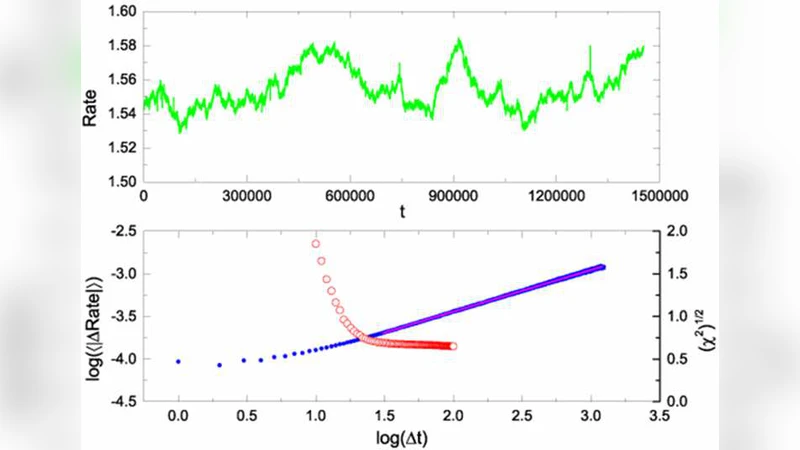
To demonstrate practical relevance, the authors analyze real financial data: the Euro‑to‑Dollar exchange rate over May–June 2008, comprising 43 trading days with many intra‑day transactions. Using case 4 sampling, they compute the rescaled range for transaction spans Δt and find that for Δt ≥ 30 the log‑log plot becomes approximately linear. An LS fit over this range yields S = 0.489 ± 0.002 and I = –0.098 ± 0.001, corresponding to a fractal dimension D = 2 – H ≈ 1.511. By applying the correction factors derived from the synthetic study (i.e., scaling the LS uncertainties by σ_S/ Sₑ and σ_I/ Iₑ, and adjusting χ²_red to the empirical values shown in Figures 3 and 8), the authors obtain more realistic error bars and confirm that the normalized residuals now follow a standard Gaussian distribution.

The paper concludes that the simple LS approach is inadequate for estimating the Hurst exponent of fractal time series because (i) the data points are correlated, (ii) the LS‑derived uncertainties are underestimated, and (iii) the slope and intercept are strongly anti‑correlated. To obtain self‑consistent estimates one must either (a) incorporate the full covariance matrix of the log‑rescaled ranges into the fitting procedure, or (b) use simulation‑based calibration tables (as provided in this work) to rescale LS uncertainties and χ² values. The authors suggest that future work could develop analytical expressions for the covariance matrix or adopt Bayesian hierarchical models that naturally account for inter‑lag correlations. Their corrected methodology, validated on both synthetic fBms and real exchange‑rate data, offers a more reliable way to quantify fractal dimensions in diverse scientific and financial contexts.