Efficient Bayesian experimentation using an expected information gain lower bound
Experimental design is crucial for inference where limitations in the data collection procedure are present due to cost or other restrictions. Optimal experimental designs determine parameters that in some appropriate sense make the data the most inf…
Authors: Panagiotis Tsilifis, Roger G. Ghanem, Paris Hajali
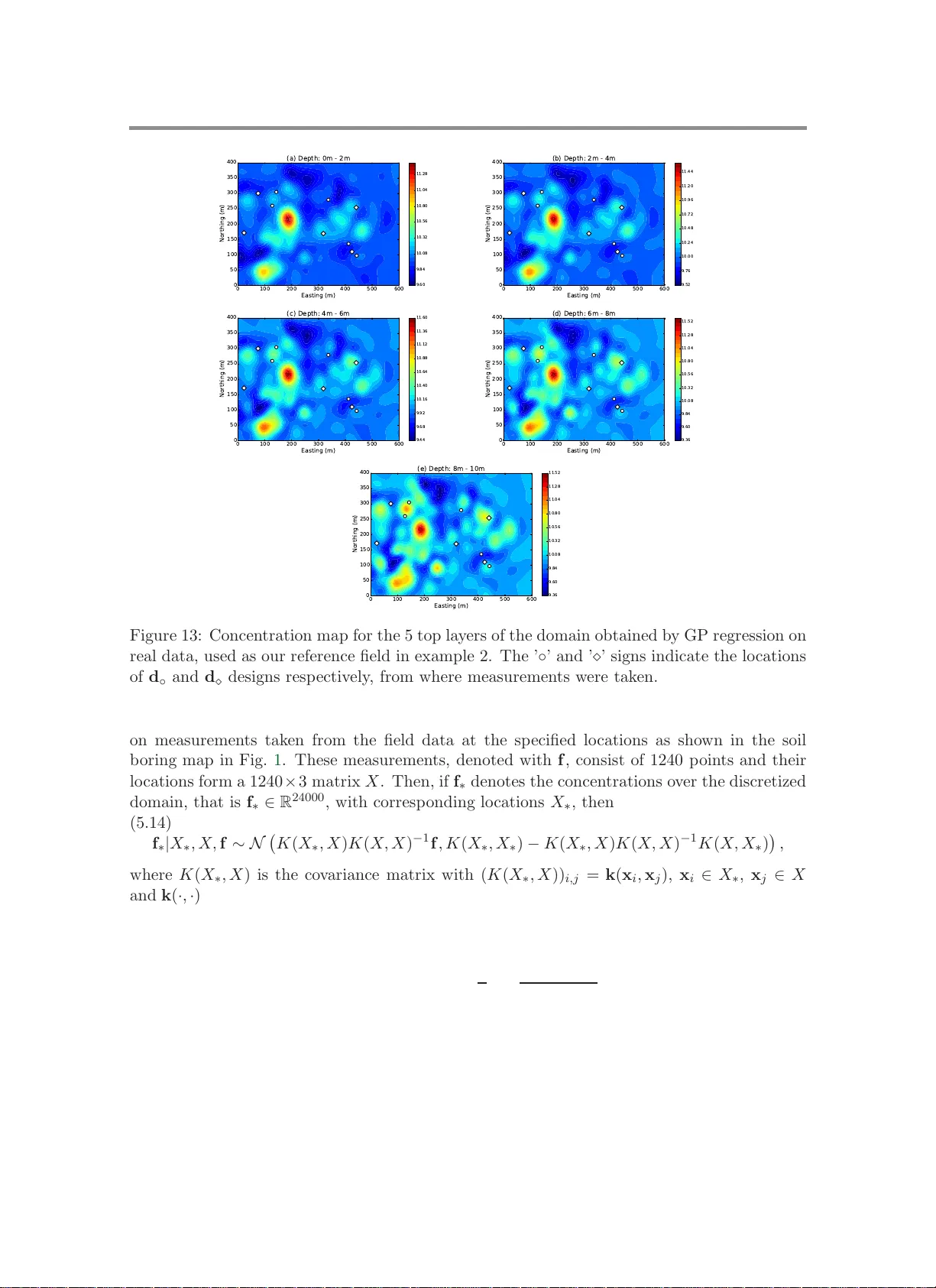
SIAM/ASA J. U NCERT AINTY Q UANTIFICA TION c xxxx So ciet y for Industrial and Applied Mathematics V ol . xx, pp. x x–x Efficient Ba y esian exp e rimentation using an exp ected info rmation gain lo w er b ound P anagiotis Tsilifis ∗ , Roger G. Gh a nem † , and Pa ris Hajali ‡ Abstract. Exp erimental design is crucial for inference where limitations in the data collection pro ced ure are present due to cost or other restrictions. Op timal experimental d esigns determine p arameters t hat in some ap p ropriate sense mak e the data the most informative possible. In a Bay esian setting this is translated to up dating to the b est possible posterior. Information theoretic arguments have led to the formation of the exp ected information gain as a design criterion. This can b e ev aluated mainly b y Monte Carlo sa mp ling and maximized by u sing sto chastic appro ximation methods, both known for b eing compu tationally exp ensive tasks. W e prop ose a framework where a lo wer bound of the exp ected information gain is used as an alternativ e d esign criterion. In addition to alleviating the computational b urden, this also add resses issues concernin g estimation bias. The problem of p ermeabilit y inference in a large contaminated area is used to demonstrate the va lidity of our ap- proac h where we emplo y the massiv ely parallel version of th e m ultiphase multicomponent sim ulator TOUGH2 to sim u late contaminan t tran sp ort and a P olyn omial Chaos ap p ro x imation of the forward mod el th at further accelerates the ob jectiv e funct ion ev aluations. The prop osed metho d ology is demonstrated to a setting where field measurements are a v ailable. Key wo rds. Ba yesian exp erimental design, Exp ected information gain, Sto chastic optimization, Polynomial Chaos, Two-phase transport AMS subject classifications. 62F15, 62K05, 86A22, 86A32 , 94A17 1. Intro duction. Remediation of a p ol lu ted subsu r face pr esen ts an increasingly common need in most urb an areas und ergoing accelerated expansions. Risks asso ciated with these p ollutan ts range from health consequences to fin ancial costs of b oth monitoring, remediation and insur ance. T he fact that the subsu rface can n ev er b e completely charac terized is a key con tributor to these r isks, and credible pr o cedures f or improving this c haracterization hav e far reac hin g consequences across the sp ectrum of constituency . What is ultimately needed is a sufficient assessmen t of the su bsurface which dep end s on the p h ysics of subsu rface fl o w and a k n o wledge of the initial conditions, and an assessment of the flow functionals that are relev ant to risk assessmen t. As a fir st step, in the presen t pap er, w e address th e issue of optimal subsur f ace c haracterization under conditions of limited resources. A v ast amoun t of researc h works h a v e b een dedicated to this c hallenge and h a v e offered application-sp ecific answers throughout the y ears with a Ba yesian decision analysis f ramew ork often b eing present. Among the earliest ones, the works b y [ 7 , 17 ], discussed the wo r th of correlated h ydraulic co n ductivit y measurement s that w as ev aluated dep ending on the rev en ue due to the resulting u ncertain t y reduction and the cost of obtaining them. In the excellen t w ork b y [ 18 ], a s equen tial samplin g metho dology wa s d ev elop ed and the issues of where to obtain the n ext sample and w hen to cease sampling w ere addressed using an analogous worth-of- ∗ Department of Math ema t ics, University of Southern Calif ornia, Los Angeles, CA 90089 ( tsilifis@usc.edu ). † Department of Civil Engineering, Universi ty of Southern Califo rnia, Los Angeles, CA 90089 ( ghanem@usc.edu ) ‡ MUREX Environmental Inc., 15375 Ba rranca Pa rkwa y , Suite K - 101, Irvine, CA 9261 8 ( paris ha jali@murexenv.co m ) 1 2 P ANAGIOTIS TSILIFIS, R OGER G. GHANEM AND P ARI S HAJALI information fr amework. More recen tly [ 11 ], a Kullbac k-Liebler formalism that maximizes the w orth of inf ormation of an experiment wa s devel op ed, and the w orth of additional observ ations c haracterized. While that w ork ignored the physics of fl o w in p orou s media by d ev eloping a kriging mo d el for the measur ed concent r ations in the su bsurface, it do es lay the f ou n dations for the presen t w ork. A common c h aracteristic in all the abov e w orks and man y th at follo wed, is that the d ata-w orth an alyses, Bay esian in nature, are divided in three main ph ases: the prior, the prep osterior and the p osterior analyses w ith the first and the last b eing the w ell kno wn steps of an y Ba y esian metho d and the second b eing the phase where the d ecisions ab out the design parameters are to b e made. This t ypically inv olv es the suggestion of a utilit y function, exp r essed often in m onetary terms that qu an tifies the worth of colle cting some sp ec ific d ata and then ev aluating the a v erage wo r th by taking the exp ectation of this function. The ab ov e mentio n ed works and numerous others [ 24 , 26 , 3 ] v erified a general conclusion: that the lo cation or any other d esign parameters c haracterizing the b est samples ma y dep en d on the mo del uncertaint y but also on the d ecision to b e mad e with th e latter factor usually add ing an economic fl a v or in the d ata w orth approac h . Although in most real-w orld problems concerning the geosciences comm un it y , this might b e an efficient w ay to address su c h issues, it is of critical imp orta n ce, fr om a mathematical p ersp ectiv e, to b e able to distinguish th e r ole of mo del un certain t y in optimal designs and n ot muc h atten tion has b een receiv ed on this dir ection. It is the p urp ose of this pap er to p resen t an app roac h to th e optimal design p roblems arising in conta min an t transp ort applications that m eets eac h p roblem’s ob jectiv es from an information theoretic p ersp ec tive, that is to exp lore the use of other design criteria as can- didates in the prep oste rior p h ase of an y data-w orth framework, that provide maximum in- formation ab out m o del u ncertain t y without b eing concerned ab out economic costs, but still pro vidin g lo w r isk resu lts for decision making. An extensiv e statistical literature is a v ailable on exp erimental design metho dologies for linear regression mo d els summ arized in [ 2 , 6 ] with criteria sta ted as functionals of the Fisher information mat r ix. Ba yesia n count erp arts of these criteria as w ell as additional design criteria for nonlinear mo d els hav e also b een suggeste d (see [ 4 ] for a review). T yp ically these are taken as the exp ectation of some appr opriately c hosen utilit y fun ctions or appro ximations of them. This is the d irection follo wed in this w ork. W e c ho ose a design criterio n for data collect ion pro cedure according to an ob jectiv e fun ction that maximizes inf orm ation gain ab out the uncertain parameters. As a natural consequen ce of dealing with realistic, complex and often high-dimensional non-linear mo d els, computationally intensiv e tec hniqu es such as the u se of mo del su rrogates and Monte Carlo m etho ds are inv olv ed in order to ev aluate and optimize the design criterion. The Ba ye sian parameter inferen ce results that are obtained f rom suc h optimal designs can then pro vide a r ational basis for decision m aking. All the ab o v e men tioned steps can b e su mmarized as shown in the flo wc hart in Fig. 2 . Th e metho dology dev elop ed in this pap er is demonstrated on an actual site sh o wn in Fig. 1 . S oil-t yp e d ata w as collected at this site at v arious depth at b oreholes located along the solid lines that criss-cross the site, as sho wn in the soil b oring map in Fig. 1 . Concent r ation v alues w ere collected at the b lac k dots throughout the site. With reference to th is sp ecific case study , the sequence of action that we in vesti gate consists of the follo wing s teps: 1. In itial s p ills are assumed to ha ve occur red at the lo cation of the storage tanks sho wn EFFICIENT BA YESIAN EXPERI MENT A TION 3 Figure 1: Aerial ph oto sho wing the lo cation of storage tanks (left) and soil borin g m ap (righ t). in Figure 1 . 2. Mean and v ariances of p ermeabilit y v alues are asso ciated to soil t yp es th roughout the site, resulting in lognormal initial probabilistic mo dels of p ermeabilities. 3. Physics of flo w through p orous media yield a corresp ond in g distribution for the con- cen tration of p ollutants thr oughout the site. 4. F or a giv en monitoring design consisting of a set o f sp ecific fiv e spatial lo cations where concen trations are to b e observ ed, a distrib u tion of these observ ables can b e obtai n ed from th e previous step. 5. F rom this distrib u tion of observ ables, th e lik eliho o d for eac h p ossible v alue of ob- serv able is calculated, and the Ba y esian p ost erior distribu tion for that observ able is ev aluat ed. Not e that at this step, no concen tration data is assumed to hav e b een collect ed yet . 6. Th e Kullbac k-Leibler (KL) d istance b et w een th e prior and the p osterior distributions is ev aluated as a measure of information gain. 7. Th e KL d istance is integrat ed o v er all p ossible v alues attained b y the observ ables at the fixed design locations. 8. Th e optimal monitoring locations are determined b y maximizing this a v eraged KL distance. 9. Measurements of p ollutan ts are tak en f r om the actual fi eld data at the optimal lo ca- tions. 10. The Ba ye sian p osterior distributions for p ermeabilitie s are calculated based on these observ ations. Th ese p osteriors pr ovide an u p dated description of the p erm eabilities throughout th e s ite and can b e used to imp ro ve the prediction of concen tration maps o v er time. While a stopping criterion for this Ba yesia n up date has b een int r o duced elsewhere [ 11 ], it is outside the scop e of the presen t in vest igation. The pap er addresses computational and algorithmic issues required for the implement ation of the ab ov e s teps and p ro vides in s igh t in to the computed optimal monitoring s tr ategie s. and is organized as follo ws. In Section 2 w e in tro du ce the d esign criterion used f or e xp erimen tal design that pro vides optimal Ba yesia n 4 P ANAGIOTIS TSILIFIS, R OGER G. GHANEM AND P ARI S HAJALI Figure 2: A fl o w chart outlining the steps in prior, p rep osterior and p osterior stages of the optimal design metho d ology . inference results and a lo wer b ound that is used as an alternativ e in the optimization p ro cedure. The sto c hastic approxima tion framework r equired f or maximizing the ob jectiv e fu nction, is describ ed in Section 3 . Section 4 pro vides a to y example in order to j ustify the use of the lo w er b ound estimate instead of the actual exp ected in formation gain as the design criterion. Then our metho dology is applied on a real site in Section 5 . Precisely , the mo del is describ ed in subsections 5.1 and 5.2 , then a surrogate is constructed in su bsection 5.3 in order to accelerate sim ulations of computationally in tensive pr o cedures. The exp erimen tal d esign analysis is p erformed in sub section 5.4 and the results are v alidated in subsection 5.5 by estimating the Bay esian u p date of the uncertain parameters based on data that is generated b oth for a hyp othetical scenario and from field measur emen ts. Our conclusions are summ arized in Section 6 . 2. Ba y esian exp erimental design. 2.1. Design criterion. Our main interest in the present work is to define and ev aluate a particular exp eriment whic h, constrained by fixed resources, will r ed uce th e prediction EFFICIENT BA YESIAN EXPERI MENT A TION 5 uncertain ty in some wel l-defi n ed optimal sense. Let d denote wh at we refer to as the set of design parameters. F or eac h c h oice of these paramete r s, the exp erimen t design is fixed. Thus d could, for instance, consist of smo othing k ernels that parameterize measurement instrumen ts. Alternativ ely , as we do in th e p r esen t work, we construe d ∈ R 2 m as a v ector that defines the spatial co ord inates in the horizon tal plane of m p oin ts at wh ic h observ ations will b e obtained. Clearly , d could also consist of nonlinear functionals. Th e n u m erical v alues of the observ ations will b e denoted b y y ∈ R m . Pr ior to conducting the exp erimen ts, y is a random vec tor. F ollo wing the exp eriment, the n umerical v alues attained by this ve ctor will b e u sed to condition the infer en ce. W e mak e the restrictiv e assumption that optimal reduction of uncertain ty in mo d el-based pred iction is attained through an optimal red uction of un certain t y in mo del parameters wh ic h w e denote b y θ . Relaxing this assump tion, w h ile n um erically tedious, do es not pr esen t conceptual difficulties. 2.1.1. Expected info rm ation gain. W e are thus in terested in inferring the u nkno w n pa- rameters θ that go v ern th e b eha vior of a physical p ro cess. W e mo del these parameters as a v ector of random v ariables. In a Ba yesia n setting, th is in ference is carried out by up dating the p rior d istr ibution p ( θ ) with a p osterior one, namely p ( θ | y , d ) , giv en that some sp ecific data y w as o b serv ed for particular d esign parameters d . The p osterio r distribution is up dated according to the rule (2.1) p ( θ | y , d ) = p ( y | θ , d ) p ( θ ) p ( y | d ) where the m ulti-dimensional in tegral, p ( y ) = R p ( y | θ , d ) p ( θ ) d θ , is referred to as the evidenc e . Using a Shannon information approac h we can define the information gain after up dating the distribution of θ to b e th e Kullback- Leibler (KL) divergence [ 20 ] of the prior and the p osterior distributions, that is (2.2) D K L [ p ( ·| y , d ) | | p ( · )] = Z Θ p ( θ | y , d ) log p ( θ | y , d ) p ( θ ) d θ . W e are in terested in quantifying the information gain b efore the d ata is actually collected. In the same spirit w e define the exp ected information gain, firs t prop osed by [ 22 ] as (2.3) U ( d ) = Z Y D K L [ p ( ·| y , d ) || p ( · )] p ( y | d ) d y = Z Y Z Θ p ( θ | y , d ) log p ( θ | y , d ) p ( θ ) d θ p ( y | d ) d y This can b e inte r preted as f ollo ws: The con tribution of an y p ossible outpu t that is u sed as a set of data y to up date to the p osterior d istribution is giv en as th e KL dive rgence of the t wo d istributions. Before the data is collected, U ( d ) provides u s with a measur e of the a v erage information to b e gained. This is a fu n ction only of the d esign parameters d . It is therefore natural to assum e that the c hoice of d ∗ that offers on aver age the most informative observ ations and th u s , is the op timal exp erimen tal design, is the one that maximizes U ( d ) and s o it s atisfies (2.4) d ∗ = arg max d ∈D U ( d ) . 6 P ANAGIOTIS TSILIFIS, R OGER G. GHANEM AND P ARI S HAJALI Ev aluatio n of the ab o v e ob jectiv e function and therefore its optimization is n ot a triv- ial task. At first, one can see that the p osterior, b eing unk n o wn b eforehand, needs to b e ev aluat ed or approximat ed. In [ 23 ], the p osterior was replaced b y its L ap lace appro ximation and U ( d ) w as estimated with a sparse quadrature r ule. In [ 31 ] an alternativ e form of th e ob jectiv e fun ction w as d eriv ed by usin g Ba yes’ rule to express the p osterior in terms of the evidence, the lik eliho o d and th e prior distr ibutions and estimates we r e prop osed v ia Mont e Carlo metho ds. In b oth app roac hes, the maxima were ident ified by using an exhaustive grid searc h o ve r the whole d esign space and limitations d ue to computational exp ense were re- p orted. Ev aluation of the d esign criterion on all p oints of the design space can easily b ecome infeasible in app licatio n s where either higher d imensional d esign parameters are inv olv ed or an exp ensiv e forward solv er is incorp orated, h ence the n eed for iterativ e searc h strategies is necessary to detect th e optimal v alue. In [ 15 , 16 ] it wa s demonstr ated that sto c hastic ap- pro ximation metho ds [ 35 ] are w ell adapted to the p resen t situation, when the Mon te Carlo estimate of the ob jectiv e is used and this is the approac h we follo w in this pap er . Ho wev er, instead of simply adapting the metho dology dev elop ed in these works, we f urther d eriv e a lo w er b ound of the exp ected in formation gain and its corresp ondin g Mont e C arlo estimate to b e maximized. The reason f or doing so is to o ve r come computational obstacles that arise from our application: The direct Mon te Carlo estimato r entai ls a discretization of the double in tegral app earing in equation ( 2.3 ) and has b een sho wn to ha ve a bias th at is inv ersely pro- p ortional to the num b er of samp les in the inner su m of the estimate, requiring a v ery large n umb er of in ner lo op samples for the b ias to b e negligible [ 31 ] (see also App endix B in [ 15 ] for a n umer ical stud y). F ur thermore, the v ariance of that estimator is con trolled only b y the n umb er of the outer loop samples. Expr essions for b ot h the bias and v ariance are give n in A . F or applications suc h as the one included in this p ap er, using tens or hundreds of thousand s samples can easily b ecome prohib itive. On the con trary , th e low er b ound deriv ed b elo w can b e easily seen to b e unbiased and its v ariance is control led by th e p ro duct of the num b er of samples used in b oth lo ops, something that allo ws us to achiev e th e same lev el of accuracy in our estimate with a m uch low er n u m b er of samples. 2.1.2. Derivation of a low er b ound. By s u bstituting p ( θ | y , d ) from eq. ?? , w e write U ( d ) = Z Y Z Θ log p ( θ | y , d ) p ( θ ) p ( θ , y | d ) d θ d y = Z Y Z Θ log [ p ( y | θ , d )] p ( y | θ | d ) p ( θ ) d θ d y − Z Y log [ p ( y )] p ( y | d ) d y and by denoting with H [ q ( ω )] = − R log [ q ( ω )] q ( ω ) d ω the en tropy of a distr ib ution q ( ω ) we tak e U ( d ) = − Z Θ H [ p ( y | θ , d )] p ( θ ) d θ + H [ p ( y | d )] . In w hat follo ws we take th e likeli h o o d as a Gauss ian d istribution with densit y p ( y | θ , d ) = (2 π ) − m/ 2 | Σ | − 1 / 2 exp − 1 2 [ y − G ( θ , d )] T Σ − 1 [ y − G ( θ , d )] . EFFICIENT BA YESIAN EXPERI MENT A TION 7 where th e mean is the mo del output G ( θ , d ) and th e cov ariance m atrix is Σ . This is a common c h oice for mo dels wh ere the observ ables y are d efined as the mo d el pred iction plu s some m easuremen t errors y = G ( θ , d ) + ǫ with the latter being normally distrib u ted with densit y N (0 , Σ ). In general, the measurement error can b e r elated to the mo del output through a pr op ortionalit y f actor or even a more complex relation which is t ypically in corp orated in the co v ariance m atrix Σ . T his implies that Σ can dep end implicitly on b oth th e uncertain and the design parameters. F or our purp oses w e mak e the rather simple assu mption th at no su ch dep en dence is inv olv ed and Σ h as fi xed entries. F urther details on the exact v alues of the co v ariance matrix in clud ing indep end ence among the measuremen t err ors is p ro vided later in our app lications. F or the ab o v e c hoice of the likeli h o o d function the en trop y can b e calculated a n d is simply H [ p ( y | θ , d )] = 1 2 { m + lo g [(2 π ) m | Σ | ] } and we finally get (2.5) U ( d ) = − 1 2 { m + lo g [(2 π ) m | Σ | ] } + H [ p ( y | d )] . A t last, using Jensen’s inequalit y , w e derive a low er b ound for U ( d ). Namely we h a v e H [ p ( y | d )] = Z Y − log [ p ( y | d )] p ( y | d ) d y ≥ − log Z Y p 2 ( y | d ) d y and we define the low er b ound of U ( d ) as (2.6) U L ( d ) = − 1 2 { m + log [(2 π ) m | Σ | ] } − log Z Y p 2 ( y | d ) d y . Note th at since the common first term of U ( d ) and U L ( d ), as they app ear in equations ( 2.5 ) and ( 2.6 ), are indep enden t of d , one ev entually n eeds only to m aximize the second term, namely the en tropy of the marginal d istribution of the data or its lo wer b ound . This idea is not new and has b ee n p r eviously used in linear regression mo dels [ 32 ] and in geoph ysical applications [ 37 ]. 2.1.3. Estimation of the low er b ound. As men tioned ab o ve , the optimization p roblem is equiv alent to minimizing U ∗ L ( d ) = Z Y p 2 ( y | d ) d y . After expanding the evidence function and writing U ∗ L ( d ) = Z Y Z Θ Z Θ p ( y | θ 1 , d ) p ( y | θ 2 , d ) p ( θ 1 ) p ( θ 2 ) d θ 1 d θ 2 d y w e can see that a Mon te C arlo estimate of the ab o ve is (2.7) ˆ U ∗ L ( d ) = 1 N M N ,M X i,j =1 p ( y i | θ j , d ) 8 P ANAGIOTIS TSILIFIS, R OGER G. GHANEM AND P ARI S HAJALI where { θ i } , { θ j } , i = 1 , ..., N , j = 1 , ..., M are i.i.d. samples from p ( θ ) and { y i } are i.i.d. samples from p ( y | θ i , d ). 3. Sto chastic optimization. 3.1. Simultaneous p erturbation sto chastic app roxi ma tion. Maximizatio n of the ob jec- tiv e fu nction derived in the ab o ve section can in general b e a difficult task. In cases where the design parameters are of high dimension or an exp ensive forw ard solv er is inv olv ed in th e ev aluat ion of U ∗ L ( d ), a direct grid searc h can easily b ec ome proh ib itiv e. S ince only a noisy estimate of the actual ob jectiv e fun ction to b e maximized is av ailable, we turn our atten tion to sto chastic appr o ximation metho ds. These are algorithms that approxima te ro ots of noisy functions and can b e used for optimization p roblems to fin d the ro ots of the grad ient of the ob jectiv e fun ction to b e optimized. This is done with an iterativ e pr o ce d ure of the general form (3.1) d k +1 = d k − a k g ( d k ) , k ≥ 0 where { a k } k ≥ 0 is a sequence of p ositiv e pre-sp eci fi ed deterministic constan ts, kn o wn also as the le arning r ate of the algorithm and g ( d ) = ∇ d U ( d ) is th e gradient of the ob jectiv e f u nction with resp ect to d . Algorithms that use an explicit expression for the gradient are called R obbins-Monr o algorithms [ 30 ] and those wh ere a finite-difference s cheme is emplo yed, are called Kiefer-W olfowitz algorithm s [ 19 ]. F or our purp oses w e use an algorithm from the Kiefe r- Wolfowitz family , namely the Simultane ous P erturb ation Sto chastic Appr oximat ion metho d (SPSA), p rop osed by Spall [ 35 , 36 ]. What mak es this metho ds attrac tive v ersu s others is the fact that only t wo forw ard ev aluations are required for th e gradien t estimat ion. The up dating step of the m etho d is giv en by (3.2) d k +1 = d k − a k ˆ g k ( d k ) , where (3.3) ˆ g k ( d k ) = ˆ U ∗ L ( d k + c k ∆ k ) − ˆ U ∗ L ( d k − c k ∆ k ) 2 c k ∆ − 1 k , 1 . . . ∆ − 1 k ,n d , (3.4) a k = a ( A + k + 1) α , c k = c ( k + 1) γ and a k , c k , α , γ are p ositive parameters whose v alues affect the con v ergence rate and the gradien t estimate. General instructions on h o w to c h o ose th e appr opriate v alues f or eac h problem are giv en in [ 36 ]. The v ectors ∆ k are random vecto rs w ith coefficients ∆ k ,i dra wn indep end en tly from an y ze r o-mean probability distribution suc h that the exp ectatio n of | ∆ − 1 k ,i | exists [ 35 ]. A common c hoice, whic h we used in our analysis, c orr esp onds to ∆ k ,i = 2( Z − 1 / 2) where Z ∼ Bernoulli( p ) with success probabilit y p = 1 2 . 4. Example: Nonlinear m o del. EFFICIENT BA YESIAN EXPERI MENT A TION 9 4.1. The model and experimental scena rios. Th e main goal in this exa mp le is to explore the accuracy of the low er b ound estimate as a su b stitute for the direct maximization of the exp ected information gain [ 15 ] and provi d e a numerical comparison of the t wo appr oac h es. This is ac h iev ed b y ev aluating the t wo ob jectiv e fu nctions for a s im p le algebraic m o del whic h is inexp ensiv e to ev aluate and is nonlin ear with resp ect to b oth the un certain and d esign parameters. Consider th us the mo del wh ere the observ able qu an tit y y is dep endent on κ and d as y ( κ, d ) = G ( κ, d ) + ǫ (4.1) = κ 3 d 2 + κe −| 0 . 2 − d | + ǫ (4.2) where G ( κ, d ) is the mo del outpu t and the n oise is taken to b e ǫ ∼ N (0 , 10 − 4 ). F or pr ior w e c ho ose initially κ ∼ U (0 , 1) and la ter on w e discuss a few more ca ses. Supp ose we h a v e con trol o v er d ∈ D where D = [0 , 1] is the design space and w e are in terested in inferrin g κ . W e explore t wo cases, first the case wh ere inference is carried out using a s ingle observ atio n of y and second the case wher e t wo observ ations of y can b e obtained, corresp onding to d ifferent v alues of d . One can think of the design p arameter d as the lo cation w h ere y is observe d . Before observin g y , we w ould lik e to know th e v alue of d that w ould make our observ ations the m ost inf orm ativ e ones. Bot h cases of this example ha ve b een studied in [ 15 ] u sing the direct Mon te Carlo estimate of U ( d ). Th e first case w as also stud ied in [ 23 ] using the Laplace appro ximation of th e p osterior distrib u tion of κ and then p erforming the in tegration with sparse quadratures. 4.2. Results. W e are using the exp ect ed inform ation gain lo we r b oun d estimate as give n in ( 2.7 ) as our criterion to determine the optimal design d f or inferrin g κ . F or comparison, w e also repro d uce the results of [ 15 ] using the exp ected information gain estimate whic h from no w on w e call double lo op M onte Carlo (dlMC) estimate. The exact expression of the dlMC estimate is giv en in A . O u r computations are p erform ed using an ensemble of samples with N = M = 10 4 for all differen t priors that w e consider b elo w, while keeping the error v ariance fixed. W e demonstrate that the t wo estimate s h are the same maxima and their graphs ha ve go o d quantitat ive agreemen t w ith the lo w er b ound p ro viding sligh tly less noisy v alues. 4.2.1. Single observation. Fig. 3 shows the v alues of estimates of U ∗ L ( d ) for the d esign of one exp eriment after using a 101-p oin t unif orm p artition on the design space D = [0 , 1] for N = M = 10 3 and for N = M = 10 4 as we ll as the estimates of dlMC. All cases sho w the existence of t wo lo cal maxima at d = 0 . 2 and d = 1. As exp ect ed, our estimate alwa ys tak es v alues sligh tly sm aller than dlMC, as the former is a lo w er b ound of the latter. Due to the fact that the first term in our estimate (the Gaussian en tropy) is a constan t, while the first term of the d lMC estimate is a Mon te-Carlo appro ximation of the very same constan t, w e observ e that the low er b ound is a smo other curv e for the same v alues of N , M . F ollo wing the slop e analysis of [ 15 ] we also pr esen t the results for tw o differen t choic es of prior, namely when κ ∼ U (0 , κ e ) and when κ ∼ U ( κ e , 1) w here κ e = (1 − e − 0 . 8 ) / 2 . 88 1 / 2 whic h is the p oint where the slop e of G ( κ, 1) b ecomes greater than the slop e of G ( κ, 0 . 2). F or the former case w e obtain a global maxim u m at d = 0 . 2 whereas for the latter, the maxim u m is at d = 1. A t some p articular p oin ts w e can observe that although our estimate is only a lo wer boun d of the 10 P ANAGIOTIS TSILIFIS, R OGER G. GHANEM AND P ARI S HAJALI 0 . 0 0 . 2 0 . 4 0 . 6 0 . 8 1 . 0 d 3 . 0 3 . 1 3 .2 3 . 3 3 . 4 ˆ U L ( d ) ( a ) κ ∼ U ( 0 , 1) D o u b l e - l o o p M C N = 1 0 3 , M = 1 0 3 N = 1 0 4 , M = 1 0 4 0 . 0 0 .2 0 . 4 0 . 6 0 .8 1 . 0 d 1 .8 1 . 9 2 .0 2 . 1 2 . 2 2 . 3 2 .4 2 . 5 ˆ U L ( d ) ( b ) κ ∼ U ( 0 , κ e ) D o u b l e - l o o p M C N = 1 0 3 , M = 1 0 3 N = 1 0 4 , M = 1 0 4 0 . 0 0 . 2 0 . 4 0 .6 0 .8 1 . 0 d 2 . 4 2 . 6 2 . 8 3 . 0 3 . 2 3 . 4 ˆ U L ( d ) ( c ) κ ∼ U ( κ e , 1) D o u b l e - l o o p M C N = 1 0 3 , M = 1 0 3 N = 1 0 4 , M = 1 0 4 Figure 3: Exp ected inform ation gain lo wer b ound s and dlMC with N = 10 4 , M = 10 4 estimated o v er D = [0 , 1] f or thr ee differen t priors. dlMC estimate, the v alue of the dlMC might fall b elo w the v alue of U ∗ L ( d ). This, in addition to the fact th at we compare noisy estimates of a deterministic q u an tit y , can also emerge as the result of the bias of dlMC whic h is not negligible for our c h oice of M (n u m b er of inner lo op samples). F or a more detailed d iscussion on the bias of d lMC for this example see [ 15 ] and f or the analytic form of th e bias see [ 31 ]. 4.2.2. Tw o observations. W e calculate th e v alues of U ∗ L ( d 1 , d 2 ) f or N = M = 10 4 o v er D × D = [0 , 1] 2 and we c omp are them with those of dlMC in Fig. 4 . S imilar qualit ative r esults as in case 1 can b e observed. F or κ ∼ U (0 , 1), th e p oin ts wh ere maxim um is attained are ( d 1 , d 2 ) = (0 . 2 , 1) and ( d 1 , d 2 ) = (1 , 0 . 2) whic h are com binations of th e lo cal m axima in th e 1-dimensional case. That means that, if tw o observ ations can b e afforded, th ey shou ld b e tak en at the p oints where lo cal m axima exist for th e one observ ation scenario. The ord er is insignifican t sin ce, as w e see, the U ∗ L ( d 1 , d 2 ) surface is symmetric w ith resp ect to th e d 1 = d 2 line. S imilar conclusions are drawn for κ ∼ U (0 , κ e ) and κ ∼ U ( κ e , 1) w here the m axima are at ( d 1 , d 2 ) = (0 . 2 , 0 . 2) and ( d 1 , d 2 ) = (1 , 1) r esp ectiv ely , as already exp ected from the resu lts of case 1. 5. Example: Case study . This second example demonstrates the app lication of the for- malism to a s u bsurf ace p ollution c haracterization pr oblem for an actual site where field data for p ermeabilit y and concentrat ions are a v ailable. EFFICIENT BA YESIAN EXPERI MENT A TION 11 0 . 0 0 . 2 0 . 4 0 . 6 0 . 8 1 . 0 d 1 0 . 0 0 . 2 0 . 4 0 . 6 0 . 8 1 . 0 d 2 κ ∼ U ( 0 , 1) 3 .1 8 0 3 .2 2 5 3 .2 7 0 3 .3 1 5 3 .3 6 0 3 .4 0 5 3 .4 5 0 3 .4 9 5 0 . 0 0 . 2 0 . 4 0 . 6 0 . 8 1 . 0 d 1 0 . 0 0 . 2 0 . 4 0 . 6 0 . 8 1 . 0 d 2 κ ∼ U ( 0 , κ e ) 2 . 0 5 0 2 . 1 2 5 2 . 2 0 0 2 . 2 7 5 2 . 3 5 0 2 . 4 2 5 2 . 5 0 0 2 . 5 7 5 0 . 0 0 .2 0 .4 0 .6 0 .8 1 .0 d 1 0 . 0 0 . 2 0 . 4 0 . 6 0 . 8 1 . 0 d 2 κ ∼ U ( κ e , 1) 2 .6 0 2 .7 2 2 .8 4 2 .9 6 3 .0 8 3 .2 0 3 .3 2 3 .4 4 (a) Low er bound estima te ˆ U L ( d ) 0 . 0 0 . 2 0 . 4 0 . 6 0 . 8 1 . 0 d 1 0 . 0 0 . 2 0 . 4 0 . 6 0 . 8 1 . 0 d 2 κ ∼ U ( 0 , 1) 3 .3 4 3 .4 0 3 .4 6 3 .5 2 3 .5 8 3 .6 4 3 .7 0 3 .7 6 0 . 0 0 . 2 0 . 4 0 . 6 0 . 8 1 . 0 d 1 0 . 0 0 . 2 0 . 4 0 . 6 0 . 8 1 . 0 d 2 κ ∼ U ( 0 , κ e ) 2 . 2 6 2 . 3 2 2 . 3 8 2 . 4 4 2 . 5 0 2 . 5 6 2 . 6 2 2 . 6 8 2 . 7 4 0 . 0 0 .2 0 .4 0 .6 0 .8 1 .0 d 1 0 . 0 0 . 2 0 . 4 0 . 6 0 . 8 1 . 0 d 2 κ ∼ U ( κ e , 1) 2 .7 6 2 .8 8 3 .0 0 3 .1 2 3 .2 4 3 .3 6 3 .4 8 3 .6 0 (b) dlMC estimate ˆ I ( d ) Figure 4: Exp ected information gain lo w er b oun d estimate and dlMC estimate with N = 10 4 , M = 10 4 for the 2-dimens ional design, estimated o ve r D = [0 , 1] 2 for differen t pr iors. 5.1. Description. W e are interested in p erforming Bay esian infer en ce on the uncertain parameters that affect the transp ort of p ollutan ts in a con taminated area. Suc h a pro cedur e will decrease the uncertain ty r egarding the exten t an d lo cation of the plume and will further affect the cost and other imp ortant asp ec ts of soil remediation. When limited resources are a v ailable for exp erimen tation and data collecti on, it is of great imp ortance to dev elop exp er- imen tal design strategies that will enhance the qualit y of d ata. Our cur r en t study concerns a contaminat ed site lo cated in Santa F e Springs, C alifornia. Previous data consisting of soil t yp es is a v ailable from b oreholes lo cated along four cross s ections across the site. Eac h b ore- hole reac hes a d ep th of 20m. Accordingly , soil t yp e is defined as a categorical v ariable with six p ossible states. T h e field and the lo cations of th e b oreholes are s ho wn in Figs. 1 and 5 (left). The a v ailable soil data is used to constru ct a domain that can b e used in our forwa r d mo d el to sim ulate th e transp ort of p ollutan ts. Th e construction of a d omain that can b e regarded as a go o d approximati on of the real situation, is ac hieved b y the stratigraphic mo d eling capabilities of the Groundw ater Modeling Sys tem (GMS) softw are [ 1 ]. More sp ecifically , us in g a stand ard in verse-dista n ce we ighting based in terp ola tion sc heme, we assign soil t yp es for all locations in the a r ea o f our in terest. The strati graphy of the resulting domain as w ell as the exten t of ea ch soil are sh o wn in Figs. 5 (right) and 6 . Next, the domain wa s d iscretized to a 40 × 60 × 10 grid wh ere eac h cell has dimensions 15 . 4m. × 6 . 7m. × 2m. an d carries the inform ation of the soil typ e present in that lo cation. Th e grid is u sed as our fi nite vo lum e d iscretizatio n in the 12 P ANAGIOTIS TSILIFIS, R OGER G. GHANEM AND P ARI S HAJALI subsequent TO UGH2 sim ulations and eac h of the six d ifferen t soil typ es presen t in our domain are assigned different p ermeabilit y v alues whic h , in our study , are considered to b e rand om and are th e only source of u ncertain t y . Figure 5: Boreholes (left) and final domain stratigraphy (righ t) with the z -axis b eing stretc hed for the s ake of illus tr ation. 5.2. Simulating flo w and transp o rt using TOUGH2. 5.2.1. EOS7r mo dule. W e emplo yed the multiphase sim u lator TO UGH2 [ 28 ] and its massiv ely p arallel ve rs ion TOUGH2-MP [ 40 ] with th e E O S7r mo du le to sim ulate groun dwa ter flo w and con taminant transp ort. TOUGH2 provides us with a finite vo lu me solve r wh ic h discretizes the mass and energy equations o ve r space and time and up d ates a set of pr imary v ariables that consist the s olution of the go verning equations by estimating the incremen ts at eac h time step with a Newton-Raphson metho d . The common mathematical form of the equations for multiphase flu id fl o w include sev eral thermophysical parameters su c h as densit y , viscosit y , enthalp y etc. whic h are determin ed by the v arious ”EOS” (equatio n -of- state) mod ules. Th e E O S7r mod ule [ 27 ] used here, is mainly intended to pr o vide radion uclide transp ort capabilit y but can b e as w ell used for transp ort of v olatile and wat er soluble orga n ic c hemicals (V OCs). Change in concen trations is caused in general for three reasons: transp ort, deca y and adsorption. V olatilization of the V OCs in all phases is mo deled by Henry’s law and o ccurs by adv ection and diffusion. Deca y is mo deled by a firs t-order deca y la w. In case of radion u clide transp ort, this is interpreted as r adioactiv e deca y bu t in the case of organic con taminan ts it can b e explained as bio degradation. Adsorption is dep end en t on th e distribution co efficien t that c haracterizes eac h ro ckt yp e. EOS7r in total can simulate tr ansp ort of five comp onen ts in a t w o-phase flow, namely water, air, brine, a paren t con taminan t and a daugh ter con taminant in aqueous and gaseous phases. 5.2.2. Santa Fe site. F or our p roblem we are inte r ested in sim ulating the spreading of organic conta min an ts in a field lo cated in San ta F e Spr ings, CA whic h is appro ximately 600 m. × 40 0 m. and only 20 m. deep. Th is is discretized in TO UGH2 to a grid consisting of 40 × 60 × 10 = 24000 activ e cells w here eac h cell has dimension 15 . 4 m. × 6 . 7 m. × 2 m. , as explained in the previous paragraph and is assigned a ro ckt yp e according to its soil t yp e. W e EFFICIENT BA YESIAN EXPERI MENT A TION 13 (a) Clay (b) Silt (c) Clay ey sand (d) Silt y sand (e) Sand with 10% silt (f ) Poor ly g raded sand Figure 6: Soil morphology of the domain. The z -axis has b ee n stretched for th e sak e of illustration. fo cus on inv estigating the propagation of u ncertain t y emerging fr om the unkn o wn p ermeabil- ities κ = ( κ 1 , ..., κ 6 ) of the six differen t soil types the are present on our site, thr ou gh th e transp ort pro cess of the V OC s . The p orosit y is take n to b e uniform φ = 0 . 35 all o ver the domain. Although w e are intereste d in the transp ort mainly of p etroleum h ydro carb ons whose w eathering pro cesses are in general kn o wn to includ e ad s orption and bio d egradation effects, for the purp oses of this study w e will consider these effects to b e of negligible imp ortance b y assignin g the distribution co efficien ts for adsorption to b e zero and th e half-life p arameter ∼ 10 50 so th at w e ha ve no deca y effects. Th us our mo del fo cuses only on the v olatilizati on prop erties of the VOCs. W e c h o ose the v alues for the molecular w eight and in verse Henr y’s constan t parameters to corresp ond to those used for describing transp ort of p etroleum hydro- carb ons and sp ecifically those that are mostly d etecte d using gas c hromatograph y tec hniqu es, named Gasoline Range Organics (GR O). Typica lly GR O are th e s ubsets of h yd r o carb ons in the C5-C12 range and in clude hydrocarb ons suc h as Benzene, T oluene, Eth ylb enzene, m-, o- and p -Xylenes, Naph thalene and Acenaphthene. T heir molecular weig hts are in the 78 − 154 grams range. In our case w e arbitrarily set th e m olecular weig ht to b e 112 . 4 grams whic h is 14 P ANAGIOTIS TSILIFIS, R OGER G. GHANEM AND P ARI S HAJALI Figure 7: Lo cations w here initial conta m in an t injections are placed. a v alue close to the a verage GR O hydrocarb on. T able 1: Material and initial parameters used in our sim ulations. P arameter Sym b ol V alue P orosit y φ 0 . 35 T ortu osity factor τ 0 0 . 1 Relativ e p ermeabilit y parameters: λ 0 . 457 - S lr 0 . 15 - S ls 1 - S g r 0 . 1 Capillary pressur e parameters: λ 0 . 457 - S lr 0 - 1 /P 0 = α/ρ w g 5 . 105 e − 4 - P max 10 7 - S ls 1 Diffusivities (all k ): gas p hase d k g 10 − 6 aqueous phase d k l 10 − 10 Molecular w eight - 112 . 4 In verse Herny’s constant - 2 . 1 · 10 − 8 Half-life parameter - 10 50 Initial pressure P (0) 1 . 013 · 10 5 Initial gas saturation S g 0 . 75 T emp erature (constant ) T 20 ◦ F or our forw ard ev aluations of the mo del with TOUGH2 we consider that only 3 com- p onents are present by assigning the b rine and daught er radionuclide mass fr actions to b e zero. W e assum e isothermal conditions with the temp erature b eing constan t at 20 ◦ C and no-flux b oundary conditions. The mathematical form ulation of the flo w and transp ort mo del is describ ed in deta il in App endix B and the v alues of the model parameters that are assumed kno wn are giv en in T able 1 . Since w e wan t the pressure and gas saturation to b e close to EFFICIENT BA YESIAN EXPERI MENT A TION 15 steady-state conditions by the time the con taminan ts are released to the ground, we first run the mo d el for a time p eriod until T = 13 . 3 yea r s, where the initial mass fractions for the con taminan ts is zero. The outp uts of pr essure and gas s atur ation are s u bsequentl y used as initial conditions for the transp ort simulat ion. W e rerun the mo d el after assigning initial aqueous phase s olub ilities for the VOC. W e denote these initial conditions with y 0 . Th eir lo cations at time t = 0 are tak en to b e approximat ely in th e areas w ere the storage tanks are lo cated as can b e seen in Fig. 7 . F or our pur p oses w e add 164 inactiv e (zero vol u me) cells to th e sur f ace la y er of our grid and initial injections are assigned. The exact v alues w ere c hosen to b e y 0 = 0 . 1 + U pp b (parts p er b illion) where U are n u m b ers rand omly generated from a Un iform distribution with supp ort on (5 · 10 − 5 , 10 − 2 ) and are considered kno wn. The transp ort sim ulation r uns for the same time p eriod as the flo w simulation. 5.3. Deve loping a surrogate mo del . Due to the complexity of our mo d el, only a single sim ulation of the tran s p ort flo w w ith TOUGH2 requires sev eral min u tes to finish. Th u s, implemen ting our experimental design framew ork, includin g the minimization of the exp ected information gain low er b ou n d with SPSA which requires thousands of ob jectiv e fun ction ev aluat ions, b ecomes impractical. It is therefore necessary to create a sur r ogate mo del that w ould pro vide us with forward ev aluations of the mo d el that are significan tly c heap er to obtain than runnin g TOUGH2. 5.3.1. The prio r and input transf o rmation. Th e un kno wn p h ysical parameters of our problem are the p erm eabilities κ = ( κ 1 , ..., κ 6 ) of the six materials making-up the s ubsurf ace at the site of in terest. W e c h o ose all κ i to b e indep end en t with a log n ormal prior distribution, that is (5.1) p (log κ i ) = N ( − 23 . 5 , 4) The choice of the mean µ = − 23 . 5 and v ariance σ 2 = 4 are made s u c h that our pr ior co vers a r ange for p ermeabilit y v alues in the order of magnitud e 10 − 8 cm 2 to 10 − 12 cm 2 whic h corre- sp onds to semi-p ervious mate r ials. W e find this a rather general prior that corresp onds s olely to our kno wledge that th e materials present in our domain are silt, cla y , silt y sand , cla yey sand, s an d w ith 10% silt and p o orly graded sand. No w if we let F ( x ) = P ( κ i ≤ x ) to b e the cumulati ve d istribution function of κ i , then we ha ve that ξ i := F ( κ i ) ∼ U (0 , 1) an d f or ξ = ( ξ 1 , ..., ξ 6 ) w e define ˆ G ( ξ ) = G ( F − 1 ( ξ ) , d ) where F ( ξ ) = Q 6 i =1 F ( ξ i ) to b e our mo del output where the in p ut is a set of 6 indep enden t standard uniform random v ariables. 5.3.2. P olynomial chaos expansion. W e mak e use of th e p rop ert y that our rand om out- put ˆ G ( ξ ) is a physical pro cess with finite v ariance, therefore it is a square-integ rable r andom field ˆ G ( ξ ) ∈ L 2 ( R m ), defined on the probabilit y sp ace ([0 , 1] 6 , F , P ) and admits a p olynomia l c haos representati on of the form [ 8 , 34 , 38 ] (5.2) ˆ G ( ξ ) = X α , | α | < ∞ p α Ψ α ( ξ ) where α = ( α 1 , ..., α d ) and α i ∈ N m for i = 1 , ..., n is a multi-index with mod ulus | α | = α 1 + ... + α n , eac h p α is a v ector in R m , ξ is a second-order r andom v ariable defined on 16 P ANAGIOTIS TSILIFIS, R OGER G. GHANEM AND P ARI S HAJALI ([0 , 1] 6 , F , P ) with v alues in R m and the f unctions Ψ α form a complete set of orthonormal functions that satisfy (5.3) E [Ψ α ( ξ )Ψ β ( ξ )] = δ αβ = δ α 1 β 1 × · · · × δ α d β d T ypically the random v ariable ξ has ind ep endent comp onent s that follo w a Gaussian, Un iform, Gamma or Beta distribu tion. The basis function then is c hosen to consist of m ultidimensional p olynomials Ψ α ( ξ ) = ψ α 1 ( ξ 1 ) × · · · × ψ α d ( α n ), where ψ α i is resp ecti vely Hermite, Legendre, Laguerre or Jacobi p olynomial s of order α i . According to the inpu t transformation in the previous paragraph, w e tak e the comp onents of ξ to b e U (0 , 1) distribu ted and therefore th e p olynomials in the expansion will b e Legendre. F or computational pu rp oses we w ork w ith a truncated v ersion of the expression ( 5.2 ) b y writing (5.4) ˆ G r ( ξ ) = X α , | α |≤ r p α Ψ α ( ξ ) . where th e n umb er of term s in the ab o v e expansions is (5.5) N p = |{ α ∈ N n , 0 ≤ | α | ≤ r }| = r X j =0 ( j + n − 1)! j !( n − 1)! . Eq. ( 5.4 ) p ro vides an accurate appro ximation of the true mo d el output y as long as the co efficien ts p α are estimated in a fashion that th ey also incorp orate a transformation of ξ to the uncertain parameters of the problem of in terest. 5.3.3. Co efficient estimation. In order for the expression ( 5.4 ) to b e of use, w e need to estimate the co efficien ts p α . This in general can b e done with v arious metho ds, mainly catego rized as in tru s iv e [ 39 ] and nonintrusiv e metho ds. W e u se n on-in trus iv e metho ds wh ich are easier to implement and more con ve n ien t w hen the forw ard simula tion is seen as a b lack b o x. P opular n onin tru s iv e metho d s include appr oximati n g the co efficient s by orthogonal pro jection of the output on the basis functions [ 9 ], whic h inv olv es calculating m ultidimens ional in tegrals. Other m etho ds calculate th e co efficien ts b y solving a linear sy s tem of equations constructed after ev aluating the mo del on a set of samples and then either in terp ol ating these p oi nts (by c ho osing collocation p oints of the p olynomial ro ots [ 21 ]) or minimizing the least s quares error [ 41 ]. The last metho d is the one adapted here, namely we estimate the co efficien ts by linear regression taking adv an tage of the linear dep end ence of ˆ G r ( ξ ) on p α . This requires the ev aluati on of ˆ G ( ξ ) at N G p oint s { ξ j } N G j =1 and th en for eac h comp onen t y c , c = 1 , ..., 24000 of the output v ector ˆ G = ( y 1 , ..., y 24000 ) T , w e solv e the system (5.6) y c = Ψ p c , where y c = [ y 1 c , ..., y N G c ] T , Ψ is the N G × N p matrix formed b y ev aluating the p olynomial basis functions at the N G selected p oin ts and p c are th e ve ctor with the unkn o wn co efficien ts. The least squares solution of ( 5.6 ) is the one th at min imizes || Ψ p c − y c || 2 and is giv en by (5.7) ˆ p c = (Ψ T Ψ) − 1 Ψ T y c EFFICIENT BA YESIAN EXPERI MENT A TION 17 pro vided that (Ψ T Ψ) − 1 exists. T h is requ ires that N G ≥ N p so that our system w ill b e o v erd etermined. Again, due to th e computationally demand in g TOUGH2 f orw ard simulato r it is impractic al to obtain tens or hundreds of thousand samp les so w e w ork with an ensem b le of N G = 1000 samples which, ev en on the massiv ely parallel v ersion of TOUGH2 (TOUGH2- MP), with a mo derate n umber of pro cessors used, tak es aroun d one w eek to b e generated. This c hoice of N G allo ws u s to calculate the co efficient s of an expansion of order up to r = 5. The p oint s { ξ j } N G j =1 w ere rand omly selecte d using Latin Hyp ercub e sampling. In f act, the 5-order p olynomial chao s exp ansion includ ed 462 co efficien ts. Th is is close to N G ≈ 2 N p whic h has b een suggested as a goo d c hoice [ 14 ]. New results concerning the stabilit y and L 2 -con v ergence of Pol yn omial Chaos approximat ions obtained via least-squares solutions h a v e b een recen tly rep orted b y [ 5 , 12 ], ho wev er suc h an analysis falls b eyond the scop e of this wo rk. 5.3.4. Go o dness of fit and truncation error. The next step after obtaining the expansion co efficien ts is to test ho w w ell ˆ G r p erforms as a surrogate. F or v alidation purp oses, we estimate the co efficien ts for r = 1 , 2 , 3 , 4 and 5 using all 1000 samp les. W e wan t to test h o w wel l the least squares solution fits the samples but also h o w close ˆ G r is to ˆ G in the L 2 sense. F or the first test we employ the common R 2 statistic kno wn also as c o e ffic i ent of deter- mination [ 33 ] and provides a go o dness-of-fit measure for our linear m o del. The statistic is defined as (5.8) R 2 c = 1 − RS S c P N G j =1 ( y i c − ¯ y c ) 2 where th e residuals sum of squares is RS S c = P N G j =1 ( y j c − y r,j c ) 2 , c = 1 , ..., 24000. F or the second test, we defin e the exp ect ed relativ e truncation error as (5.9) e c = E [ |G c ( ξ ) − y c ( ξ ) | 2 ] E [ |G c ( ξ ) | 2 ] = R [0 , 1] n |G c ( ξ ) − y c ( ξ ) | 2 p ( ξ ) d ξ R [0 , 1] n |G c ( ξ ) | 2 p ( ξ ) d ξ , c = 1 , ..., 24000 where p ( ξ ) = 1 is the join t distribution of in d ep endent U (0 , 1)’s. The ab ov e can b e estimated as (5.10) e c ≈ P 1000 j =1 |G c ( ξ j ) − y c ( ξ j ) | 2 P 1000 j =1 |G c ( ξ j ) | 2 , c = 1 , ..., 24000 . Fig. 8 shows the b o xplots of the R 2 statistic, obtained from all comp onents G , of the expansions of order r = 1 , ... 5 (left) and the b o xplots of the r elativ e err ors for eac h order r = 1 , ..., 5 and for all the comp onents of G (righ t). Regarding the R 2 statistic and particularly for r = 5 the m edian is 0 . 986 and the lo w er qu artile is ab o v e 0 . 96 giving us a go o d fit for the 75% of the exp ansions along the d omain. A thorough lo ok sho wed that the remaining outputs including outliers for w hic h the fit is not stable corresp ond to p oin ts of the d omain that are in the b otto m la ye r and along the east b ound ary . Regarding the exp ec ted truncation err or and sp ecifically for the expansions of order 5 the median is 3 . 1 · 10 − 4 and the upp er quant ile is 10 − 2 giving u s go o d appr o ximations in th e L 2 sense. Again the trun cation error in creases for th e p oint s in the b ottom la yers. T o ensure that our exp erimen tal design metho dology 18 P ANAGIOTIS TSILIFIS, R OGER G. GHANEM AND P ARI S HAJALI implemen ted in the n ext paragraph is un affected b y p ossible instabilities of the Pol yn omial Chaos expansions, the mo del outp uts pro d uced for the b ottom lay er of our domain we r e not in vol ved in our study . 1 2 3 4 5 P o l y n o m i a l o r d e r r 0 . 0 0 .2 0 .4 0 .6 0 .8 1 . 0 R 2 R 2 st a t i sti c 1 2 3 4 5 P o l y n o m i a l o r d e r r 0 .0 0 .2 0 .4 0 .6 0 .8 1 .0 e c R e l a t i v e e r r o r Figure 8: Bo xplots of the R 2 statistic (left) and relativ e errors (right ) of the p olynomial c haoses for all comp onents of the output G ( ξ ), of order r = 1 , ..., 5. 5.4. Experimental design. 5.4.1. Design settings. As men tioned ab o v e, our main goa l is to p erf orm Ba yesian infer- ence on the p ermeabilit y parameters that will pro vide us a tight er p osterior that will decrease the un certain t y ab out the tr ue v alues of the soil p erm eabilit y . This will further enh ance our current kno wledge ab out the plum e lo cation an d extent that can p otent ially result in devel- oping cost-efficien t remediation str ategies. In order to achiev e such a goal, we are seeking the b est lo cations from where data sh ould b e collected by employing the exp ecte d information gain lo w er b ound as our design criterion. Unlik e th e analysis of the nonlinear algebraic mo d el it is clearly un dersto o d that in th is case, design of a single exp erimen t, that is design for the colle ction of a sin gle datum w ould not ha ve imp orta nt effe cts in the inference procedu r e and it is never p erf orm ed in practice. In our setting w e consider that for any lo cation in the ( x, y )-plane we can observe the concen trations y from the first 5 lay ers of our domain, that is up to 10m. depth, so 5 d ata p oint s are a v ailable from eac h location. Without any lo ss of generalit y in our metho d w e c ho ose to find the design of exp eriment s consisted of the 5 b est lo cations in the ( x, y )-plane from where d ata will b e collect ed sim u ltaneously to b e used for inference. This is a mo derate c hoice whic h app ea r s to b e satisfact ory in ord er to v alidate our m etho d. F urther ev aluation of the optimal n umb er of data p oint s is b ey ond the scop e of the present study . The design parameters therefore are d = ( d 1 ,x , d 1 ,y , d 2 ,x , d 2 ,y , ..., d 5 ,x , d 5 ,y ) where ( d i,x , d i,y ) ∈ D 0 = [0 , 600] × [0 , 400], i = 1 , ..., 5 and th e design space for our problem is D = D 5 0 . The observ ations y are sub ject to additional measurement noise as indicated fr om our Gaussian lik eliho o d f u nction N ( y | ˆ G ( ξ ) , Σ ) inv olv ed in th e exp ected information gain lo wer b ound deriv ation. Here we hav e substituted ou r f orward solv er G ( κ , d ) with the p olynomial c haos surrogate ˆ G ( ξ ). The co v ariance mat r ix has b een c hosen to b e Σ = σ 2 I 25 with σ 2 = 10 − 2 . This is a rather simp le choice that guaran tees that measurement errors are indep en d en t. A EFFICIENT BA YESIAN EXPERI MENT A TION 19 0 1 0 0 2 0 0 3 0 0 4 0 0 5 0 0 6 0 0 E a st i n g ( m ) 0 5 0 1 0 0 1 5 0 2 0 0 2 5 0 3 0 0 3 5 0 4 0 0 No r th i n g ( m ) 0 2 0 4 0 6 0 8 0 1 0 0 1 2 0 ( a ) N = M = 10 0 2 0 4 0 6 0 8 0 1 0 0 0 1 0 0 2 0 0 3 0 0 4 0 0 5 0 0 6 0 0 E a sti n g ( m ) 0 5 0 1 0 0 1 5 0 2 0 0 2 5 0 3 0 0 3 5 0 4 0 0 No r th i n g ( m ) 0 2 0 4 0 6 0 8 0 1 0 0 1 2 0 ( b ) N = M = 100 0 2 0 4 0 6 0 8 0 1 0 0 0 1 0 0 2 0 0 3 0 0 4 0 0 5 0 0 6 0 0 E a sti n g ( m ) 0 5 0 1 0 0 1 5 0 2 0 0 2 5 0 3 0 0 3 5 0 4 0 0 No r t h i n g ( m ) 0 2 0 4 0 6 0 8 0 1 0 0 1 2 0 ( c ) N = M = 1000 0 2 0 4 0 6 0 8 0 1 0 0 Figure 9: Scatter plots of the optimal p oin ts d i for all optimization solutions d ∗ of the SP SA algorithm. T h e red transparent area s denote the lo cations of the sources, plotted for compar- ison of the p atterns. more soph isticated c h oice wo u ld b e to tak e the standard deviation to b e prop ortional to the observ able qu an tit y σ = a ˆ G c ( ξ , d ) where a is some prop ortionalit y factor. W e a void this c hoice as it imp lies the d ep endence of the error on the design p arameters w hic h con tradicts our assu mptions for the lo w er b ound deriv ation. 20 P ANAGIOTIS TSILIFIS, R OGER G. GHANEM AND P ARI S HAJALI 5.4.2. Results. W e run the SPSA algo r ith m in order to find d that minimizes ˆ U ∗ L , there- fore maximizes the low er b ound estimat e. T o assess the p erformance of the algorithm, w e r u n sev eral cases w here the choice s of N and M in the Monte Carlo lo op v ary . It is easy to see that the v ariance of our estimator is (5.11) v ar h ˆ U ∗ L ( d ) i = 1 N M v ar [ p ( Y | κ , d )] whic h sh o ws th at N and M ha ve the same con trib ution in con trolling the v ariance, therefore we tak e them equ al. As s tated previously , our estimator is unbiased, u nlik e the d lMC estimator, so an extremely large v alue for M is not n ecessary as it is for dlMC to main tain a lo w bias. W e consid ered three different cases where N = M = 10 , 100 and 1000. Since the resu lts of SPSA are noisy , in ord er to b etter ev aluate the p erformance of the algorithm w e obtain the results of 100 ind ep endent run s for eac h case. F or the fi r st t wo cases w e r un the algorithm for a total of 10 4 ev aluat ions of the ob jectiv e fun ction and for the last case we run for 5 · 10 3 ev aluat ions. It app ears that these c hoices are rather h igh since the iterate s are stabilized muc h earlier main taining a lo w iteration error. The resulting 5-tuples of p oin ts in D 0 are sho wn all together in a tota l of 500 p oin ts in Fig. 9 , for all thr ee cases. This giv es us a qualitativ e idea ab out w h ere the exp ect ed information gain is maximized and so data sh ould b e coll ected fr om. Th e formation of a certain p attern as N , M are increased is obvio u s and the optimal p oin ts ap p ear to b e very close to where the con taminan t sources w ere placed. A t the same time v arious p oints that app ear to b e outliers are also pr esent, a c h aracteristic b ehavio r of the SPS A algorithm. The case N = M = 10 p articularly sh o ws all p oin ts widely sp read all ov er D 0 and one can only distinguish the tw o areas aroun d ( x, y ) = (150 , 250) and around ( x, y ) = (450 , 100) where more p oin ts are accumulate d . The cases N = M = 100 and N = M = 1000 p ro vide v ery similar conclusions with the ma jorit y of the runs ha ving conv erged at v ery sp ecific lo cations, close to the actual con taminan t sources, forming a clear pattern with the main difference that in the th ird case the p oint s are eve n more concen trated and less outliers are p resen t. F or a more qu an titativ e argument w e also p r esen t the exact v alues of ˆ U ∗ L ( d ) as we ll as those of (5.12) ˆ U L ( d ) = − 1 2 { m + lo g [(2 π ) m | Σ | ] } − log 1 N M N ,M X i,j =1 p ( y i | κ ij , d ) calculate d at all outcomes d ∗ of our r u ns. These v alues quantify the information gain that eac h d esign is expected to offer and at the end, if we had to c ho ose only one design, this should b e the design th at pr o vides the largest v alue. Th is time, for diagnostic reasons an d in ord er to provide a measur e of comparison, we wa nt to ha ve a fixed accuracy for the estimates and w e use the same num b er of samples N = M = 1000 for the ev aluatio n of the tw o ob jectiv e functions on all p oin ts. Their v alues are all shown in the histograms p r esen ted in Fig. 10 . Again there is a significan t difference b et w een the qu alit y of the r esults of the first case with that of th e last tw o cases for b oth fu nctions. F or ˆ U ∗ L ( d ), the first case giv es us designs that whose v alues v ary in a range from 0 . 1 · 10 8 to 6 · 10 10 (observ e that the x -axis of the histogram is an order of magnitude larger than the rest) w ith a large num b er of them b eing a w a y from EFFICIENT BA YESIAN EXPERI MENT A TION 21 0 1 2 3 4 5 6 F i n a l ˆ U ∗ L ( d ) v a l u e 1 e 1 0 0 2 4 6 8 1 0 1 2 C o u n t ( a ) N = M = 10 − 3 −2 − 1 0 1 2 3 F i n a l ˆ U L ( d ) v a l u e 0 2 4 6 8 1 0 1 2 C o u n t ( b ) N = M = 10 0 . 0 0 .2 0 .4 0 .6 0 .8 1 .0 1 .2 1 .4 1 .6 1 . 8 F i n a l ˆ U ∗ L ( d ) v a l u e 1 e 9 0 2 4 6 8 1 0 1 2 C o u n t ( c ) N = M = 100 − 3 −2 − 1 0 1 2 3 F i n a l ˆ U L ( d ) v a l u e 0 2 4 6 8 1 0 1 2 C o u n t ( d ) N = M = 100 0 . 0 0 .5 1 . 0 1 .5 2 .0 F i n a l ˆ U ∗ L ( d ) v a l u e 1 e 9 0 2 4 6 8 1 0 1 2 C o u n t ( e ) N = M = 1000 − 3 −2 − 1 0 1 2 3 F i n a l ˆ U L ( d ) v a l u e 0 2 4 6 8 1 0 1 2 C o u n t ( f) N = M = 1000 Figure 10: Histograms of the ˆ U ∗ L ( d ) (left) and ˆ U L ( d ) (righ t) v alues for all optimal p oints d ∗ . the minimum v alue. The imp ression one might get for this case is that c hances are few that the optimization will yield an optimal design solution and n ot just an outlier. The other t wo cases pro vide similar results w ith the third b eing, as exp ected, b etter than the second, in the sense that the op timal p oints are even more concen trated around the m inim um v alue. F or completeness we present also ˆ U L ( d ) whic h is tec hn ically nothing else but the n egativ e logarithm of ˆ U ∗ L ( d ), s h ifted by a constant . In the fir st case, the v alues co v er a r an ge f r om − 3 to 2 . 5 with a mean around 0. The last tw o cases giv e u s again similar r esults with b ot h histograms co v ering v alues from around 1 to 3 . 5, a muc h narro wer in terv al than th e first case. Again we can see that the third case is sligh tly b etter than the second w here w e see that the unimo dal stru cture of the histogram is more concentrat ed on higher v alues close to 3 wh ic h implies that a few m ore runs even tually conv erged to the global maxim um. 22 P ANAGIOTIS TSILIFIS, R OGER G. GHANEM AND P ARI S HAJALI T able 2: The ( x, y )-co ordinates of the 5-p oint designs d ◦ and d ⋄ and their ˆ U L ( d ) v alues. d 1 d 2 d 3 d 4 d 5 ˆ U L ( d ) d ◦ (127 . 9 6 , 259 . 65) (442 . 5 9 , 97 . 05) (143 . 22 , 304 . 41 ) (337 . 1 1 , 279 . 02 ) (412 . 26 , 135 . 8 6) 3 . 698 d ⋄ (22 . 95 , 171 . 37) (75 . 36 , 300 . 00) (318 . 58 , 169 . 2 7) (425 . 06 , 109 . 96) (4 41 . 00 , 253 . 70) 0 . 286 5.5. Ba y esian up date of log ( κ ) . I n ord er to v alidate our metho dology and demonstrate the significance of the exp erimental design analysis deve lop ed ab o v e, w e p er f orm Ba ye sian inference based on t wo different designs that are selected according to the resu lts of th e previous s ection. More precisely , data f rom tw o differen t s ets of 5 p oints, d en oted with d ◦ and d ⋄ , is co llected and used to up date the probabilit y d istribution of κ . S p ecifically , d ◦ is selected among the 100 optimal designs that w ere appro ximated by S PSA in the previous section, for N = M = 1000 and is the one that ac h ieved the maximum ˆ U L ( d ) v alue, so based on the previous analysis it is the design that is exp ect ed to yield the b est p osterior. Th e second design d ⋄ , c hosen for comparison only , was arbitrarily selected among the optimal designs that w ere returned b y SPSA using the p o or estimate with N = M = 10 and has a m uc h low er ˆ U L ( d ) v alue, therefore it is expected to up date to a wider p osterior. T he exa ct lo cation of the p oint s for eac h set and their ˆ U L ( d ) v alues are shown in T able 2 . Since the p osterior distributions cannot b e calculated explicitly , we u s e Markov Chain Monte Carlo (MCM C) metho d s to d ra w samples from them. MCMC metho ds r ely on gener- ating a sequence of random v ariables based on a Marko v Chain that co nv erges to a sta tionary distribution π ( y ), called the target distrib ution and therefore th e sequence generated after a burn -in p erio d, can b e though t of as follo wing the stationary distribution π . T o av oid strong auto correlation among the samp les, appropriate th inning an d tun ing of the algorithm is re- quired. A p ow erful MCMC metho d is the Metrop olis-Hastings (MH) algorithm that w as fi rst prop osed by Metrop ol is [ 25 ] and later generalized b y Hastings [ 13 ]. The MH algorithm at an arbitrary step generates a new s amp le y f rom a pr op osal distribu tion q ( x, y ) giv en that x is the last accepted sample and accepts it with probabilit y (5.13) α ( x, y ) = m in 1 , π ( y ) q ( x, y ) π ( x ) q ( y , x ) . In our case we use the ad ap tive version of the MH algorithm as dev elop ed in [ 10 ] with a Gauss ian as the prop osal distrib ution where its co v ariance m atrix is up dated at eac h step taking into accoun t all the previous samp les that ha ve b een drawn. Th is implies that the c hain is non-Mark o vian, h o w ever it has b een pro v ed that it has the correct ergodic prop erties. The adaptive MH (aMH) algo r ithm provides faster co nv ergence to the target distribu tion and ac hiev es lo we r auto correlation among the samp les w ithout v ery large thinn ing. Belo w we explore t wo cases where in the first d ata is observ ed from a reference field that is asso ciated with one sp ec ifi c realizatio n of the m o del outpu t w hile in the second, data is observ ed f rom a reference fi eld that is constructed usin g Gaussian pro cess (GP) regression on measuremen ts tak en from the real site. 5.5.1. Case 1: Reference data generated from prio r. Here we assu me a h yp othetic al situation where the real p ermeabilit y v alues are those d ispla y ed on T able 3 . Ou r mo del’s EFFICIENT BA YESIAN EXPERI MENT A TION 23 0 1 0 0 2 0 0 3 0 0 4 0 0 5 0 0 6 0 0 E a sti n g (m) 0 5 0 1 0 0 1 5 0 2 0 0 2 5 0 3 0 0 3 5 0 4 0 0 North i n g ( m) (a ) De p th : 0 m - 2 m 0.00 0.75 1.50 2.25 3.00 3.75 4.50 5.25 6.00 0 1 0 0 2 0 0 3 0 0 4 0 0 5 0 0 6 0 0 Ea sti n g ( m) 0 5 0 1 0 0 1 5 0 2 0 0 2 5 0 3 0 0 3 5 0 4 0 0 North i n g ( m) (b ) De p th : 2 m - 4 m 0.0 0 0.7 5 1.5 0 2.2 5 3.0 0 3.7 5 4.5 0 5.2 5 6.0 0 6.7 5 0 1 0 0 2 0 0 3 0 0 4 0 0 5 0 0 6 0 0 E a sti n g (m) 0 5 0 1 0 0 1 5 0 2 0 0 2 5 0 3 0 0 3 5 0 4 0 0 North i n g ( m) ( c ) De p th : 4 m - 6 m 0 1 2 3 4 5 6 7 0 1 0 0 2 0 0 3 0 0 4 0 0 5 0 0 6 0 0 Ea sti n g ( m) 0 5 0 1 0 0 1 5 0 2 0 0 2 5 0 3 0 0 3 5 0 4 0 0 North i n g ( m) (d ) De p th : 6 m - 8 m 0.0 0.9 1.8 2.7 3.6 4.5 5.4 6.3 7.2 0 1 0 0 2 0 0 3 0 0 4 0 0 5 0 0 6 0 0 Ea sti n g ( m) 0 5 0 1 0 0 1 5 0 2 0 0 2 5 0 3 0 0 3 5 0 4 0 0 No r th i n g ( m) (e ) De p th : 8 m - 1 0 m 0 .0 0 .9 1 .8 2 .7 3 .6 4 .5 5 .4 6 .3 7 .2 8 .1 Figure 11: Concentrat ion map for the 5 top lay ers of the d omain used as the reference field in example 1. The ’ ◦ ’ and ’ ⋄ ’ signs indicate th e lo cations of d ◦ and d ⋄ designs r esp ectiv ely , from w here measuremen ts were taken. T able 3: T ru e v alues of κ and log ( κ ) u sed for generating the data in case 1. i log κ i κ i (cm 2 ) 1 − 22 . 195 2 . 295 · 10 − 10 2 − 20 . 791 9 . 346 · 10 − 10 3 − 21 . 567 4 . 300 · 10 − 10 4 − 25 . 193 1 . 145 · 10 − 11 5 − 25 . 272 1 . 058 · 10 − 11 6 − 24 . 610 2 . 050 · 10 − 10 output for those v alues ca n b e directly ev aluated and the 5 top la y ers are disp lay ed in Fig. 11 . With this reference fi eld assum ed to b e our ”realit y”, w e collect data from the lo cations indicated at designs d ◦ and d ⋄ and use them for ou r compu tations. W e generate 50000 samp les with a 10000 -samp le bu rn-in p erio d and w e retain a samp le ev ery 5 steps. After 8000 samples are obtained, histograms of th eir v alues are sh own in 24 P ANAGIOTIS TSILIFIS, R OGER G. GHANEM AND P ARI S HAJALI Fig. 12 . Note that the histograms displa y the marginal distribution of eac h log κ i , i = 1 , ..., 6 whic h are no longer indep enden t themselv es, ho wev er comparison of the histograms f or eac h case toge th er with their priors and the true v alue giv es us an idea ab out the differen t r esu lts obtained for eac h d esign. As exp ected, w e observe that d ◦ pro vides narro wer p osteriors that d ⋄ . T his can b e observed particularly on log κ 2 and log κ 5 and in a smaller scale on log κ 1 , log κ 3 and log κ 4 . The p osterio r s of log κ 6 for b oth designs do not disp la y any significan t discrepancy fr om the prior but ev en in this case the on e corresp onding to d ◦ app ear to b e sligh tly decen tralized tow ards the true v alue. In addition, for d ⋄ three p osteriors, namely log κ 2 , log κ 5 and log κ 6 retain their gaussian b ell- sh ap ed form and it seems that almost no new information has b een gained ab out their v alues. This is actually a consequ ence of the fact that the corresp onding soils (silt y sand, sand with 10% silt and cla y) are not presen t in the lo cations where the d ata w as co llected from, for this design. Note that cl ay is p resen t in the lo we r la y ers of our domain and n ot muc h information is gained ab out it fr om d ◦ either. An other general c haracteristic is that, ev en for the soils for w h ic h b oth designs pro vide similar p oste r iors, th e maxim um a p osteriori v alues of d ◦ sho w excellen t agreement with the true v alues while th ose of d ⋄ sho w a sligh t d iscrepancy wh ic h makes them inappropriate for estimation. Ove r all, w e conclude that the design d ◦ pro vides significan tly b ette r inference results that those pro vided b y d ⋄ and this conclusion can b e generalized for the comparison of d ◦ with any other d esign that ac hiev es a lo we r ˆ U L ( d ) v alue. − 3 0 −2 8 − 2 6 −2 4 −2 2 − 2 0 −1 8 − 1 6 V a l u e 0 . 0 0 . 1 0 . 2 0 . 3 0 . 4 0 .5 0 . 6 p ( l og( κ 1 ) | y ) l og( κ 1 ) − 3 0 −2 8 − 2 6 −2 4 −2 2 −2 0 − 1 8 −1 6 V a l u e 0 . 0 0 . 1 0 .2 0 . 3 0 . 4 0 . 5 p ( l og( κ 2 ) | y ) l og( κ 2 ) −3 0 −2 8 −2 6 − 2 4 − 2 2 −2 0 −1 8 −1 6 V a l u e 0 . 0 0 . 2 0 .4 0 . 6 0 . 8 1 . 0 1 . 2 1 . 4 1 . 6 1 . 8 p ( l og( κ 3 ) | y ) l og( κ 3 ) − 3 0 −2 8 − 2 6 −2 4 −2 2 − 2 0 −1 8 − 1 6 V a l u e 0 . 0 0 . 1 0 . 2 0 . 3 0 . 4 0 .5 0 . 6 0 . 7 p ( l og( κ 4 ) | y ) l og( κ 4 ) − 3 0 −2 8 − 2 6 −2 4 −2 2 −2 0 − 1 8 −1 6 V a l u e 0 . 0 0 . 1 0 .2 0 . 3 0 . 4 0 . 5 0 . 6 p ( l og( κ 5 ) | y ) l og( κ 5 ) −3 2 − 3 0 −2 8 −2 6 − 2 4 −2 2 − 2 0 −1 8 −1 6 V a l u e 0 . 0 0 0 .0 5 0 . 1 0 0 .1 5 0 . 2 0 0 .2 5 0 . 3 0 p ( l og( κ 6 ) | y ) l og( κ 6 ) Figure 12: Comparison of th e histograms of th e marginal p osteriors of all log ( κ i ), i = 1 , ..., 6 for the designs d ◦ (green) and d ⋄ (red). Th e red curve indicates their common prior distr ib ution and th e dashed blac k line ind icates th e tru e v alue used to generate the d ata. 5.5.2. Case 2: Reference data fr om field measurements. In this case, the data used in the lik eliho o d fun ction whic h is incorp orated in the accepta n ce probabilit y through Ba y es’ rule, is tak en f r om a reference concen tration fi eld, that w as generated by GP regression based EFFICIENT BA YESIAN EXPERI MENT A TION 25 0 1 0 0 2 0 0 3 0 0 4 0 0 5 0 0 6 0 0 E a sti n g (m) 0 5 0 1 0 0 1 5 0 2 0 0 2 5 0 3 0 0 3 5 0 4 0 0 North i n g ( m) (a ) De p th : 0 m - 2 m 9.60 9.84 10.08 10.32 10.56 10.80 11.04 11.28 0 1 0 0 2 0 0 3 0 0 4 0 0 5 0 0 6 0 0 Ea sti n g ( m) 0 5 0 1 0 0 1 5 0 2 0 0 2 5 0 3 0 0 3 5 0 4 0 0 North i n g ( m) (b ) De p th : 2 m - 4 m 9.5 2 9.7 6 10 .00 10 .24 10 .48 10 .72 10 .96 11 .20 11 .44 0 1 0 0 2 0 0 3 0 0 4 0 0 5 0 0 6 0 0 E a sti n g (m) 0 5 0 1 0 0 1 5 0 2 0 0 2 5 0 3 0 0 3 5 0 4 0 0 North i n g ( m) ( c ) De p th : 4 m - 6 m 9.44 9.68 9.92 10.16 10.40 10.64 10.88 11.12 11.36 11.60 0 1 0 0 2 0 0 3 0 0 4 0 0 5 0 0 6 0 0 Ea sti n g ( m) 0 5 0 1 0 0 1 5 0 2 0 0 2 5 0 3 0 0 3 5 0 4 0 0 North i n g ( m) (d ) De p th : 6 m - 8 m 9.3 6 9.6 0 9.8 4 10 .08 10 .32 10 .56 10 .80 11 .04 11 .28 11 .52 0 1 0 0 2 0 0 3 0 0 4 0 0 5 0 0 6 0 0 Ea sti n g ( m) 0 5 0 1 0 0 1 5 0 2 0 0 2 5 0 3 0 0 3 5 0 4 0 0 No r th i n g ( m) (e ) De p th : 8 m - 1 0 m 9 .36 9 .60 9 .84 1 0.08 1 0.32 1 0.56 1 0.80 1 1.04 1 1.28 1 1.52 Figure 13: C oncen tration map for the 5 top la y ers of the d omain obtained b y GP regressio n on real data, used as our reference field in example 2. Th e ’ ◦ ’ and ’ ⋄ ’ signs indicate the lo cations of d ◦ and d ⋄ designs resp ectiv ely , from wh ere m easur emen ts w ere taken. on measurements taken from the field d ata at th e sp ecified lo cations as sh o wn in the soil b oring map in Fig. 1 . T hese measurement s, d enoted with f , consist of 1240 p oi nts and their lo cations form a 1240 × 3 matrix X . Then, if f ∗ denotes the co ncentratio n s o v er the discretize d domain, that is f ∗ ∈ R 24000 , with corresp ondin g lo cations X ∗ , then (5.14) f ∗ | X ∗ , X , f ∼ N K ( X ∗ , X ) K ( X, X ) − 1 f , K ( X ∗ , X ∗ ) − K ( X ∗ , X ) K ( X, X ) − 1 K ( X , X ∗ ) , where K ( X ∗ , X ) is the co v ariance matrix with ( K ( X ∗ , X )) i,j = k ( x i , x j ), x i ∈ X ∗ , x j ∈ X and k ( · , · ) denotes some appropr iately c hosen k ernel (for more details on the deriv ation of this conditional distribution one can see [ 29 ]). I n our case we chose a squ ared exp onentia l kernel, giv en as (5.15) k ( x , x ′ ) = σ 2 exp " − 1 2 3 X n =1 ( x n − x ′ n ) 2 ℓ 2 n # whic h w as fit to the data with v ariance σ 2 = 5 and correlatio n lengths ( ℓ 1 , ℓ 2 , ℓ 3 ) = (30 , 30 , 10). Our r eferen ce field, consists of the mean ¯ f = K ( X ∗ , X ) K ( X, X ) − 1 f and the v alues of the 5 26 P ANAGIOTIS TSILIFIS, R OGER G. GHANEM AND P ARI S HAJALI − 3 0 −2 8 −2 6 −2 4 −2 2 − 2 0 −1 8 −1 6 −1 4 V a l u e 0 . 0 0 . 2 0 . 4 0 . 6 0 . 8 1 .0 1 .2 p ( l og( κ 1 ) | y ) l og( κ 1 ) − 3 0 −2 8 − 2 6 −2 4 −2 2 −2 0 − 1 8 −1 6 V a l u e 0 . 0 0 .2 0 . 4 0 . 6 0 . 8 1 . 0 1 . 2 1 .4 p ( l og( κ 2 ) | y ) l og( κ 2 ) −3 0 −2 8 −2 6 − 2 4 − 2 2 −2 0 −1 8 −1 6 V a l u e 0 1 2 3 4 5 6 7 p ( l og( κ 3 ) | y ) l og( κ 3 ) − 3 4 − 3 2 − 3 0 −2 8 − 2 6 −2 4 − 2 2 −2 0 −1 8 − 1 6 V a l u e 0 . 0 0 .5 1 .0 1 . 5 2 . 0 2 . 5 3 . 0 p ( l og( κ 4 ) | y ) l og( κ 4 ) − 3 4 − 3 2 − 3 0 − 2 8 −2 6 − 2 4 − 2 2 − 2 0 −1 8 −1 6 V a l u e 0 . 0 0 .2 0 . 4 0 . 6 0 . 8 1 . 0 1 . 2 1 .4 1 . 6 p ( l og( κ 5 ) | y ) l og( κ 5 ) −3 2 −3 0 −2 8 −2 6 −2 4 −2 2 −2 0 −1 8 −1 6 − 1 4 V a l u e 0 . 0 0 . 1 0 . 2 0 . 3 0 .4 0 . 5 p ( l og( κ 6 ) | y ) l og( κ 6 ) Figure 14: Comparison of th e histograms of th e marginal p osteriors of all log ( κ i ), i = 1 , ..., 6 for the designs d ◦ (green) and d ⋄ (red). The red curv e indicates their co mm on prior distribu tion. top la y ers are sho wn in Fig. 13 . Again, w e s et th e p ost eriors with p ( κ | y , d ◦ ) and p ( κ | y , d ⋄ ) as our target distributions and this time we generate 100000 samples w ith a 10000-sample bur n-in p erio d and we re- tain a sample ev ery 5 steps. After 18000 samples are obtained, histograms of the m arginal distributions of eac h log κ i , i = 1 , ..., 6, are sho wn in Fig. 14 . Again, w e observ e that d ◦ pro vides narro we r p osteriors than d ⋄ for most of the cases. This can b e observ ed particularly on log κ 1 , log κ 4 and log κ 5 . The p osterior of log κ 6 for the optimal design is almost identica l to its prior w hic h implies that nothing n ew has b een learned ab out its true v alue. As in the previous example, this is du e to the fact that th e corresp ond ing soil (cla y) is not present in the lo cations where the data wa s collec ted, for th is design (recall that cla y is present in the lo w er la yers of our d omain). In this case, s in ce our data is obtained from a pro cedure other than ev aluating our forwa rd mo d el, it cannot b e seen as a d irect output of it and generally w e do not exp ect to obs er ve uniqueness of the input parameters that can p otenti ally giv e rise to our measurements. Th is is r eflected by the f act that differen t designs giv e p osteriors that seem to concen trate around differen t v alues. Bay esian inference how ev er, still provides us with informativ e resu lts as w e obser ve the p osterior distribu tions to b e m u ch further a wa y from the priors, thus lea r ning something ab out ho w close our m o del and our prior assumptions are to the actual realit y . 6. Conclusions . W e p resen ted an exp erimen tal d esign framew ork that fo cuses on p r o vid- ing optimal solutions to the design problem in terms of maximizing the information on mo del parameters from Ba y esian inference. This w as ac h iev ed b y emplo ying an inform ation theoretic criterion, namely the exp ected r elativ e entrop y b et w een th e prior and the p osterior distrib u- EFFICIENT BA YESIAN EXPERI MENT A TION 27 tions of the unkno w n parameters. An additional reform ulation of the design criterion through the deriv ati on of a lo wer b oun d, w as of great importance in order to address biasedness issues as well as allevia te the compu tational b urden asso ciated with optimization. The framewo r k w as applied to a real-w orld problem: The pr ob lem of p ermeabilit y id en tifi- cation in con taminated soils in the presence of exp erim ental field data. Th e forw ard mo d el in this case consisted of a system of differen tial equat ions that describ e con taminan t transp ort in p orous media, namely a tw o-component, t w o-phase flo w-and-trans p ort mo del that pro vides as its output the concen trations of th e p ollutan ts at the time wh en data is collec ted. The design parameters consist of multiple lo cations w here the concen trations will b e measured. In the present setting, with the analogous adopted co de (TOUGH2) used as a blac k b o x sim ulator, no deriv ativ e in formation w as av ailable to the optimization pro ce ss . Th e SPSA algorithm, in add ition to add r essing this iss u e also seemed to accelerate conv ergence to the optimal so- lutions. T o fu rther redu ce the compu tational cost, constru ction of a mo del su r rogate was of crucial imp ortance since th e imp lemen tation of suc h a pro cedu re would b e impractical oth- erwise. Finally , our metho dology was v alidate d after th e inferen ce r esults sho wed that the data collected at the optimal design lo cations we r e muc h more informativ e than the d ata ob- tained from other arbitrarily c h osen p oin ts, in the sense th at they r esulted in muc h narro wer p osteriors, thus gaining more knowle d ge ab out the true s itu ation in th e sub s urface. W e ob- serv e from our analysis that, und er limited resources, th e p er f ormance of a Bay esian up date dep ends significan tly on the location of data acquisition. This highligh ts the need for optimal monitoring la y outs in order to manage en vironmental risks under economic constraints. App endix A. Comparison of the exp ected information gain estimates. A.1. The double-lo op Monte-Carlo estimate. The exp ected information gain can b e rearranged in the form I ( d ) = Z Y Z K { log [ p ( y | κ , d )] − log [ p ( y | d )] } p ( y | κ , d ) p ( κ ) d κ d y and can b e ev aluate d by u s ing Mon te Carlo metho ds with ˆ I ( d ) = 1 N N X i =1 log p ( y i | κ i , d ) − log 1 M M X j =1 p ( y i | κ i,j , d ) , where { κ i } , { κ ij } , i = 1 , ..., N , j = 1 , ..., M are i.i.d. samples f r om p ( κ ) and { y i } are i.i.d. samples from p ( y | κ i , d ). A.2. Prop erties of t he estimates. Th e p rop erties of ˆ I ( d ) are explored in [ 31 ]. Precisely it is sho wn that the v ariance is prop ortional to v ar h ˆ I ( d ) i ∝ A ( d ) N + B ( d ) N M and th e bias is prop ortional to B ias h ˆ I ( d ) i ∝ C ( d ) M , 28 P ANAGIOTIS TSILIFIS, R OGER G. GHANEM AND P ARI S HAJALI where A ( d ), B ( d ) and C ( d ) are terms th at dep end on the lik eliho o d and evidence fun ction. Clearly , as mentioned ab o v e, N con trols the v ariance and M con trols the bias. F or ˆ U ∗ L ( d ) w e hav e v ar h ˆ U ∗ L ( d ) i = 1 N M v ar [ p ( y | θ , d )] and th e bias is trivially zero, whereas for ˆ U L ( d ) w e hav e v ar h ˆ U L ( d ) i = v ar log 1 N M N ,M X i,j =1 p ( y i | θ i,j , d ) ≈ v ar " log U ∗ L ( d ) + 1 N M P N ,M i,j =1 p ( y i | θ i,j , d ) − U ∗ L ( d ) U ∗ L ( d ) # = v ar " 1 N M P N ,M i,j =1 p ( y i | θ i,j , d ) − U ∗ L ( d ) U ∗ L ( d ) # = 1 N M v ar [ p ( y | θ , d )] U ∗ L ( d ) 2 , where th e second line follo ws after 1st-order T a ylor expansion ab out U ∗ L ( d ) and B ias h ˆ U L ( d ) i = E h ˆ U L ( d ) − U L ( d ) i = E − log 1 N M N ,M X i,j =1 p ( y i | θ i,j , d ) + log U ∗ L ( d ) ≈ 1 N M v ar [ p ( y | θ , d )] U ∗ L ( d ) 2 , where the third line follo ws after a 2nd-order T a ylor exp ansion. Here the v ariance and the bias of the low er b ound are con trolled by b oth N and M . App endix B. Governing equations for flo w and tra nsp o rt in a p orous medium. B.1. Balance equations. The general mass- and energy balance e qu ations in a multico m- p onent (NK comp onen ts) multiphase problem are given as dM k dt = ∇ · F k + q k , k = 1 , ..., N K, where k is lab eling the mass comp onent up to a to tal of N K , M represents mass or energy p er v olume, F r epresen ts mass or heat flu x and q d en otes sinks or sources. In some formulations, suc h as in TOUGH2, an int egral expression is used in the f orm d dt Z V n M k dV n = Z Γ n F k · n d Γ n + Z V n q k dV n , k = 1 , ..., N K where V n is an arb itrary sub domain of the flo w system and Γ n its closed b oundary surface, n is a vec tor normal on the su rface elemen t d Γ n p oint in g in w ard into V n . If TOUGH2 is EFFICIENT BA YESIAN EXPERI MENT A TION 29 used for the numerical solution of the gov erning equations, mo du le EO S 7r pr o vides consisten t c haracterization of th e constitutiv e equations, allo wing a v alue of NK as high as 5 (water, air, brine, p aren t radionucli d e, daughter radionuclide). In out problem, a zero sou r ce term is assum ed r esu lting in q = 0 and the conta min ant sources in the mo del are tak en to b e lo calized on th e sur face, at pr e-assigned spatial lo cations shown in Fig. 7 . In a TOUGH2 formalism, these sources are mo deled as injections in attac hed zero-v olume blo c ks connected to the grid blo c ks wh ere the sour ce is assu med to b e. The m ass accum ulation cond ition f or the k th comp onent is M k = φ X β S β ρ β X k β where the summation is tak en o ver the fluid phases (liquid, gas, non-aqueous ph ase liquids). Only liquid and gas phase are considered in our case. Th e p orosit y is den oted b y φ , S β is the saturation of ph ase β (take s v alues from 0 to 1), ρ β is the density of p hase β and X k β is the mass fraction of comp onen t k pr esent in phase β . The advecti ve mass fl ux is giv en as F k adv = X β X k β F β and in dividual phase fluxed are giv en by a multiphase version of Darcy’s la w: F β = ρ β u β = − κ κ r β ρ β µ β ( ∇ P β − ρ β g ) . Here u β is the Darcy v elo cit y (v olume fl ux) in phase β , κ is the absolute p erm eabilit y , κ r β is relativ e p ermeabilit y to p hase β , µ β is viscosit y and P β = P + P cβ is the fl uid pressure in ph ase β , w hic h is the sum of the pressur e P of a reference ph ase (usually tak en to be th e gas phase) and the capillary p r essure P cβ ( ≤ 0), g is th e v ector o f gra vitational accele r ation. V ap or pressur e low ering d ue to capillary and ph ase adsorption effects is mo deled b y Kelvin’s equation P ν ( T , S l ) = f V P L ( T , S l ) P sat ( T ) where f V P L = exp M w P cl ( S l ) ρ l R ( T + 273 . 15) is the v ap or p ressure lo wering factor. Ph ase adsorption is n eglecte d . The saturated v ap or pressure of bulk aqueous phase is denoted by P sat , P cl is the d ifference b et wee n aqueous and gas phase pressures, M w is the molecular w eight of w ater and R is the un iv ersal gas constant. T emp erature T is assum ed constant. The absolute p ermeabilit y of the gas phase in creases at low pressur es according to the relation giv en by Klin ken b erg κ = κ ∞ 1 + b P 30 P ANAGIOTIS TSILIFIS, R OGER G. GHANEM AND P ARI S HAJALI where κ ∞ is the p ermeabilit y at ”infinite” p ressure and b is the Klink enb erg parameter. In addition to Darcy’s flo w, mass flux o ccurs by molecular diffusion according to f k β = − φτ 0 τ β ρ β d k β ∇ X k β . Here d k β is the molecular diffusion co efficien t for comp onen t k in phase β , τ 0 τ β is the to r tuosit y whic h includes a p orous medium d ep enden t factor τ 0 and a co efficient that dep ends on ph ase saturation S β , τ β = τ β ( S β ). Finally , the total mass flux is finally giv en by F k = F abd + X β f k β . B.2. Relative p ermeability mo del. Th e relativ e p ermeabilit y is assu med to follo w th e v an Genuc h ten-Mualem mo del w hic h for liquid is κ r l = ( √ S ∗ h 1 − 1 − S ∗ 1 /λ λ i 2 , S l < S ls 1 , S l ≥ S ls and f or gas is κ r g = ( 1 − κ r l , if S g r = 0 1 − ˆ S 2 1 − ˆ S 2 , if S g r > 0 sub ject to restrictio n 0 ≤ κ r l , κ r g ≤ 1. Here S ∗ = ( S l − S lr ) / ( S ls − S lr ) and ˆ S = ( S l − S lr )(1 − S lr − S g r ). B.3. Capilla ry p ressure mo del. F or the capillary pressu r e w e use th e v an Genuc h ten function giv en as P cap = − P 0 S ∗− 1 /λ − 1 1 − λ sub ject to restrictions − P max ≤ P cap ≤ 0. Again S ∗ is defined as for the relativ e p ermeabilit y . B.4. P arameters. T able 1 disp la ys the n ominal v alues assigned to all parameters requir ed according to the ab o ve go v erning equ ations. It is imp ortan t also to note the f ollo wing for our sim ulation: 1. The mobilities are upstream we ighted. 2. The p er m eabilities are harmonic weigh ted. 3. Mo dule EOS7r currently neglects brine and daughte r radionuclide, resulting in a 3- comp onen t flow. 4. Adsorption effects are neglected. 5. Bio degradation effects are neglected. REFERENCES [1] Aquav eo, L.L.C., 2007. Gr oundwater Mo deli ng System V ersion 6.5.6, build date, May 27, 2009, UT, USA . EFFICIENT BA YESIAN EXPERI MENT A TION 31 [2] A.C. Atkinson and A .N. Donev. Optimum exp erimental design with SAS . Oxford Statistical Science Series, Oxford Universit y Pres s, 2007. [3] D.A. Ba´ u and A.S. May er. O ptimal d esign for pump-and -treat under u ncertain hydraulic condu ctivity and plume distribution. Journal of Contaminant Hydr olo gy , 100: 30–46, 2008. [4] K. Chaloner and I. V erdinelli. Bay esian exp erimen tal design: a review. Statistic al Scienc e , 10:273–304, 1995. [5] A. Cohen, M.A. Dave n p ort, and D. Leviatan. On the stabilit y and accuracy of leats squares approxima - tions. F oundations of Computational Mathematics , 13:81 9–834, 2013. [6] V.V. F edoro v . The ory of optimal exp eriments . Academic Press, New Y ork, 197 2. [7] R.A. F reeze, B. James, J. Massmann, T. Sp erling, and L. Smith. H ydrogeological decision an alysis, 4: The concept of data worth and its use in the developmen t of site inv estigation strategies. Gr ound Water , 30 :574–588, 1992. [8] R.G. Ghanem and P .D. S panos. Sto chastic finite elements: A sp e ctr al appr o ach, r evise d e dition . Dov er Publications Inc, 2012. [9] D.M. Ghiocel and R.G. Ghanem. Sto c h astic finite element analysis of seismic soil structure interaction. Journal of Engine ering Me chanics , 12 8:66–77, 2002. [10] H. Haario, E. S ak sman, and J. T amminen. A n adaptive metrop olis algorithm. Bernoul li , 7:223–242, 2001. [11] H. Haddad-Zadegan, R. Ghanem, and P . Ha jali. Data w orth analysis in spatial prediction and soil remediation. In G. Deod atis and B. Ellingwood , editors, ICOSSAR’13: International Conf er enc e on Structur al Safety and R eliabili ty , Columbia Universit y , June 16 -20 2013. [12] J. Hampton and A . Do ostan. Coherence motiv ated sampling and conv ergence analysis of least-squares p olynomial c haos regression. arXiv pr eprint, arXiv:1410.1931 , 201 4. [13] W.K. Hastings. Monte carlo sampling meth o ds using marko v chains and their applications. Biometrika , 57:97–1 09, 1970. [14] S. Hosder, R .W. W alters, and M Bal ch. Efficient sampling for non- intrusiv e p olynomial chaos applications with multiple un certain input v ariables. In 9th AIAA Non-Deterministic Appr o aches Confer enc e , 2007. [15] X. Huan and Y. Marzo uk . Sim ulation-based opt imal ba yesian ex p erimen tal design for nonlinear systems. Journal of Computational Physics , pages 288–317, 2013 . [16] X. Hu an and Y . Marzouk. Gradien t-b ased sto chas t ic optimization metho ds in bayes ian exp erimental design. I nternational Journal for Unc ertainty Quantific ation , 4:47 9–510, 2014. [17] B.R. James and R.A. F reeze. The wo rth of d ata in predicting aquitard contin u it y in hydrogeologi cal design. W ater R esour c es R ese ar ch , 29:20 49–2065, 1993. [18] B.R. James and S .M. Gorelic k. Wh en enough is enough: The worth of monitoring data in aquifer remediation design. Water R esour c es R ese ar ch , 30:3 499–3513, 1994. [19] J. Kiefer and J. W olfo witz. Stochastic estimation of a reg ression function. T he Annals of Mathematic al Statistics , 23 :462–466, 1952. [20] S. Kullback and R.A. Leibler. On information and sufficiency . The Ann al s of Mathematic al Statistics , 22:79–8 6, 1951. [21] H. Li and D. Zhang. Probabilistic collocation method for flow in p orous media: Comparisons with other stochastic methods. Water R esour c es R ese ar ch , 43:4 4–56, 2007. [22] D. V. Lindley . On a measure of the info rmation p rovided b y an exp eriment. T he Annals of Mathematic al Statistics , 27 :986–1005, 1956. [23] Q. Long, M. Scavino, R. T empone, and S. W ang. F ast estimation of ex p ected information gains for bay esian exp erimental desig n s based on laplace approximations. Computational Metho ds in Appli e d Me chanics and Engine ering , 259, 2013. [24] J. Ma ssmann and R.A. F reeze. Groundwater contamination fro m waste management sites: The in terac- tion betw een risk-based engineering design and regulatory p olicy:1. metho dology . Water R esour c es R ese ar ch , 23 :351–367, 1987. [25] N. Metrop olis, A.W. Rosenbluth, M.N. R osen blu t h, A.H. T eller, and E. T eller. Equ ations of sta te calcu- lations b y fa st computing mac hines. Journal of Chemic al Physics , 21:10 87–1091, 1953. [26] T. Norb erg and L. Ros´ en. Calculating th e optimal num b er of contaminan t samples by means of data w orth analysis. Envir onmetrics , 17:705–719, 2006. [27] C. Oldenburg and K. Pruess. EOS7R: R adionuclide tr ansp ort for TOUGH2 . Berk eley , California, No vem- 32 P ANAGIOTIS TSILIFIS, R OGER G. GHANEM AND P ARI S HAJALI b er 1995. R ep ort LBL-3486 8. [28] K. Pruess, C. Olden b urg, and G. Mo ridis. TOUGH2 User’s guide, V ersion 2 . Berkeley , California, 1999 . Rep ort LBNL-4313 4. [29] C.E. R asm ussen and C.K.I. Williams. Gaussian pr o c esses for machine le arning . The M I T Press, 2006. [30] H. Robbins and S. Monro. A stochastic approximati on metho d. The Annals of Mathematic al Statistics , 22:400– 407, 1951. [31] K.J. Ryan. Estimating exp ected information gains for exp erimental designs with app lication to the random fa tigue-limit mo del. Journal of Computational and Gr aphic al Statistics , 12:5 85–603, 2003. [32] P . Sebastiani and H.P . Wy nn. Maximum entropy sampling and optimal bay esian exp erimental design. Journal of the R oyal Statistic al So ciety. Series B: Statistic al Metho dolo gy , 62:14 5–157, 2000 . [33] G.A.F. Seber and A.J. Lee. Line ar r e gr ession analysis, se c ond e dition . John Wiley and Sons, 2003. [34] C. Soize and R. Ghanem. Ph ysical systems with random uncertainties: Chaos representations with arbitrary probabilit y measure. SIAM Journal of Scientific Computing , 26(2): 395–410, 2004. [35] J.C. Spall. Multiv ariate sto chastic approximatio n using a simultaneous p erturb ation gradien t approxi- mation. I EEE T r ansactions on Automatic Contr ol , 37, 1992. [36] J.C. Sp all. Implementation of the sim u ltaneous p erturb ation algorithm for stochastic optimization. I EEE T r ansactions on A er osp ac e and Ele ctr onic Systems , 34 , 1998. [37] J. v an den Berg, A. Curtis, and J. T ramp ert. Optimal nonlinear b a yesian exp erimental design: an application to amplitude v ersus offset experiments. Ge ophysic al Journal International , 155:411–42 1, 2003. [38] D. Xiu and G.E. Karniadakis. The wiener-ask ey p olynomial c haos for stochastic differen tial equations. SIAM Journal of Scientific Computing , 24:619–644, 2002. [39] D. X iu and G.E. Karniadakis. Modeling uncertaint y in fl o w sim ulations via generalized polynomial chaos. Journal of Computational Physics , 187 :137–167, 2003. [40] K. Zhang, Y.S. W u, and K . Pruess. User’s guide for TO U GH2-MP - A massively p ar al lel version of the TOUGH2 c o de . Berkel ey , California, 2008. Rep ort LBNL-315E. [41] Y. Zhang and N .V. Sahinidis. Uncertain ty q u antificati on in co 2 sequestration using surrogate mo dels from polynomial c haos expansion. Industrial & Engine ering Chemistry R ese ar ch , 52:3121– 3132, 2012.
Original Paper
Loading high-quality paper...
Comments & Academic Discussion
Loading comments...
Leave a Comment